Stated Choices and Simulated Experiences: Differences in the Value of Travel Time and Reliability - Stephane Hess
←
→
Page content transcription
If your browser does not render page correctly, please read the page content below
Stated Choices and Simulated Experiences:
             Differences in the Value of Travel Time and Reliability

                                          Muhammad Fayyaz a
                                           Michiel Bliemer a,*
                                             Matthew Beck a
                                             Stephane Hess b
                                             Hans van Lint c

               a
                Institute of Transport and Logistics Studies, University of Sydney, Australia
   b
       Choice Modelling Centre, Institute for Transport Studies, University of Leeds, United Kingdom
        c
          Department of Transport and Planning, Delft University of Technology, the Netherlands
                                          *
                                            corresponding author

Abstract
Surveys with stated choice experiments (SCE) are widely used to derive values of time and reliability
for transport project appraisal purposes. However, such methods ask respondents to make
hypothetical choices, which in turn could create a bias between choices made in the experiment
compared to those in an environment where the choices have consequence. In this paper, borrowing
principles of experimental economics, we introduce an incentive compatible driving simulator
experiment, where participants are required to experience the travel time of their chosen route and
actually pay any toll costs associated with the choice of a tolled road. In a first for the literature, we
use a within respondent design to compare both the value of travel time savings (VTT) and value of
travel time reliability (VOR) across a typical SCE and an environment with simulated consequence.
Given the importance of VTT and VOR to transport decision making and the difficulty in estimating
VOR using revealed preference data, our results are noteworthy and emphasise that more research
on this topic is imperative. We provide suggestions on how the results herein may be used in future
studies, to potentially reduce hypothetical bias that may be exhibited in SCE.

Keywords
Hypothetical bias; Route choice behaviour; Stated choice experiments; Incentive compatible driving
simulator experiments; Value of travel time; Value of travel time reliability.

                                                    1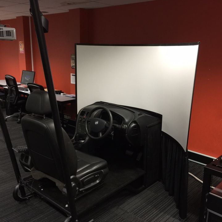
1. Introduction
1.1. The Value of Time and Reliability
Route choice has been a topic of study for many decades in order to better understand the importance
of various route attributes and to forecast behaviour in networks for transport planning and
management purposes. Key in route choice analysis is the ability to derive the value of travel time
(VTT) and the value of travel time reliability (VOR). VTT is the monetary value drivers assign to travel
time changes, and VOR is the monetary value assigned to a change in travel time variability
(unreliability). For the past five decades, the VTT has been considered an important value in transport
policies and transport projects appraisal (Abrantes & Wardman, 2011). VTT serves two purposes,
namely (i) as an input variable in cost-benefit analysis (CBA) of transport infrastructure projects, and
(ii) as an explanatory variable in transport forecasting models (Shires & de Jong, 2009). More recently
(for the last two decades), VOR has also received considerable attention in the CBA of transport
projects and policies (de Jong & Bliemer, 2015).

Given the importance of these inputs to fundamental transport decisions, there has similarly been
much research into data types used to examine route choice decisions. Broadly speaking, the two
types of data are stated preference (SP) and revealed preference (RP). SP data typically are collected
with a stated choice experiment (SCE), in which respondents are asked to make choices in a series of
hypothetical choice tasks. In contrast, RP data consists of route choices observed in the field, for
example where drivers are tracked using mobile phones or other Global Positioning System (GPS)
devices, remote sensing, or using driver-reported route information in interviews and questionnaires.
VTT and VOR are often estimated using SP rather than RP data1. For example, in the UK, a large number
of SCEs were designed for estimating VTT and VOR for different transport modes and trip purposes
(Hess et al., 2017), and similar SP data collections have been conducted in many other countries.

While it is typically assumed that behaviour captured by SCEs reflects real-world behaviour, the
hypothetical nature of SCEs may lead to biased results (Beck et al., 2016; Fifer et al., 2014). One of the
potential reasons for hypothetical bias in typical SCEs is that “participants may not experience strong
incentives to expend the cognitive efforts needed to provide researchers with an accurate answer”
(Ding et al., 2005, p. 68). A SCE would therefore be incentive compatible only if it provides an incentive
for participants to nudge them to truthfully reveal their preference towards an attribute. Experiments
designed specifically to be incentive compatible are widely conducted in experimental economics and
are often referred to as an economic experiment. Conversely, the tendency to simplify SCE settings, a
practice that prevails despite extensive criticism (cf. Hess et al. 2020a), may lead to respondents
enhancing the information in an unobserved manner to make up for the lack of experienced stimuli.

1.2. Contribution of this Research
Given that differences may exist between values calculated on stated preference versus revealed
preference data, research that seeks to examine this discrepancy is imperative given the importance
of VTT and VOR to transport decision making. This research is, however, somewhat lacking. Following
an extensive literature review on the comparison of stated preference (SP) and revealed preference
(RP) data in the context of transportation, there are only two papers in the field that make the
comparison between the two types of data with respect to VTT and VOR.

1
 Some exceptions exist (e.g., Carrion & Levinson, 2013; Fezzi et al., 2014; Prato et al., 2014), though historically
RP data is rarely used to estimate VTT and VOR because many contexts cannot be (easily) examined in a real-
world driving study (e.g., certain roads may not yet exist, certain toll levels may not yet exist). It is also very
challenging to reconstruct objective or perceived route travel time distributions on road networks. More
recently, there has been a renewed interest in using RP data for VTT research (e.g., Varela et al., 2018).

                                                         2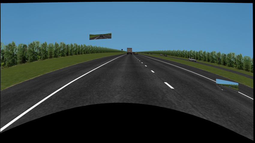
Brownstone & Small (2005) and Small et al. (2005) both make use of the same dataset wherein self-
reported RP choices with regards to use of a tolled express lane on two highways in the US. By
assuming that drivers know the distribution of travel times across days (which is a strong assumption),
for any given time of day, they can measure VTT and VOR as preferences about this distribution. As
with many studies that seek to examine VTT and VOR in a revealed preference context, Brownstone
and Small (2005) acknowledge difficulties in data collection resulting in only one of the routes being
able to satisfactorily identify coefficients of unreliability, with these results being sensitive to
specification. In both studies, the SP survey asked people to choose among situations in which they
trade off total travel time, the fraction of travel time in congested conditions, and trip cost between
two otherwise identical routes. The SP tasks were generic across respondents and not pivoted around
their actual experiences, though effort was made to segments split travellers into nine bands of total
travel time. With regards to the data, there are 55 respondents from whom both RP and SP data was
collected.

Brownstone and Small (2005) found differences in VTT estimated from both experimental treatments,
and conclude that the examination of VOR is promising, but more research be done in studying this
value. Small et al. (2005) use the same data and through a different modelling approach find that scale
difference between SP and RP models was significant and that VTT and VOR were substantially
underestimated based on SP data when compared to RP. A key limitation of both these studies,
however, is that the SP and the RP data cannot be directly compared because the alternatives and
levels shown are different across both data sources. As acknowledged by the authors, these
differences can lead to travel time misperceptions or inconsistent behaviours.

To accommodate for this, Krčál et al. (2019), citing our original conference presentation2 with
preliminary findings of the research discussed herein, present an examination of VTT where the choice
faced in the SP and RP setting were identical to allow for a more direct comparison. Note that the
authors refer to RP results in their study, but the outcome was still experienced in a laboratory setting.
While it is common for this type of experiment to be referred to as RP in experimental economics
given that the monetary incentive is real, we argue that such data should be considered SP because
the consequence is unlike that which would be experienced in a real world setting, despite an
associated consequence with respect to time. Nonetheless, they find that VTT in the SP experiment is
significantly lower than that revealed by the RP component of the experiment. Krčál et al. (2019) do
not investigate VOR and instead of making all choices consequential, they randomly select only one
choice task out of 80 to be consequential.

To better understand hypothetical bias, we need to understand the sources of hypothetical bias in a
stated choice experiment. Is bias caused by the absence of consequences? Or because the
environment is not realistic? Or perhaps because people provide socially desirable responses that do
not reflect their actual behaviour? The presence of hypothetical bias varies across disciplines, for
example in health economics it has been found that stated choice experiments have little to no
hypothetical bias, while there is ample evidence in the environmental economics and consumer
economics literature that the absence of consequences is an important source of hypothetical bias
(Haghani et al., 2021). Haghani et al. (2021) distinguishes five classes of choice data, ranging from Class
I (least realistic) data collected via typical non-consequential choice experiments to Class V (most
realistic) data obtained via naturalistic choice observations. Class II refers to data from (partially)
consequential choice experiments, Class III is associated with quasi-revealed or lab-in-the-field choice
experiments, and Class IV refers to self-reported (or agent-aware) choice observations in the field.
Existing studies on hypothetical bias in choice experiments have compared Class I data with data in a

2
  Early results of our study were presented at the 15th International Conference on Travel Behaviour Research in
July 2018 in Santa Barbara, USA.

                                                       3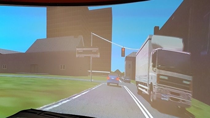
higher (more realistic, less hypothetical) class as benchmark, Table 1 summaries these studies based
on the review of 57 articles across four applied economics domains in Haghani et al. (2021). This
illustrates that there exist four studies in transport that have compared data from a typical
hypothetical choice experiment with true choice observations (Class V) to demonstrate that
hypothetical bias exists (Ghosh, 2001; Brownstone et al., 2003; Brownstone and Small, 2005; Small et
al., 2005). However, it should be noted that these four studies used the same data set, illustrating that
availability of Class V data is rare.

     Table 1 Empirical studies into hypothetical bias of non-consequential choice experiments

 Applied economics domain                   Class II       Class III   Class IV   Class V       Total
 Transport economics                           2              5            3         4           14
 Environmental/resource economics             12              --           3         --          15
 Consumer economics                           13              2           --         3           18
 Health economics                              --             --          10         --          10

Our study contributes to the transport literature by investigating whether the absence of
consequences in stated choice experiments are a source of hypothetical bias, i.e., we make a
comparison with Class II data. Currently, only two such studies have been conducted in transport,
namely Hultkrantz and Savsin (2017) and Krčál et al. (2019), who both identified significant bias in VTT
due to consequences. However, they used a between-respondent design such that differences may
be due to sample differences across the two data collection types. Our study adopts a within-
respondent design to provide further evidence that the absence of consequences in a stated choice
experiment is a source of hypothetical bias, not only in the context of VTT but also with respect to
VOR.

Thus, the motivation for our study is to contribute to this very small body of research by examining
drivers’ route choice behaviour in both a stated preference experiment and an economic driving
simulator experiment (DSE) that requires respondents to experience the travel times, costs, and travel
time unreliability consequences of their choices in a more realistic setting. In particular, our
experimental treatment ensures that the same respondents complete identical choice tasks in both
experimental treatments, and in addition we are able to estimate VOR in not only the SP context, but
also in the simulated RP experiment. To the best of our knowledge, this is the first study of its kind
and this paper makes an additional contribution to the existing literature by being the first to use an
economic DSE to estimate VTT and VOR measures in a route choice context.

1.3. Outline of the Paper
The remainder of the paper is organised as follows. To help position the identified contribution of this
research, we first provide a literature review of data collection techniques in a route choice context
and their features. This is followed by an overview of the two experiments that are used to collect
data, which is then followed by a discussion of the relatively novel experimental design that
underpinned the values embedded in the stated choice experiments. We then provide information
about the sample and some preliminary analysis, before looking at the results of comprehensive
model estimation. Finally, we conclude with a discussion of the limitations of the current study, the
over-arching outcomes of this research for the literature, and suggest future directions for research
based on this analysis.

                                                       4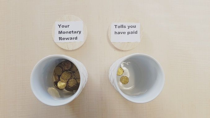
2. Literature Review
Given the vast amount of literature on the collection of choice data, we limit this literature review to
data collection techniques in the transport domain, with particular reference to route choice, VTT and
VOR. We discuss these data collection methods in the light of the trade-off between (external) validity
(do the data reflect real behaviour) versus the degree of experimental control in collecting the data,
illustrated in Figure 1, in which field data (RP) and experimental data (SP) are placed along both these
axes. With respect to field data, the analyst has little control over the environment in which the data
is collected, but the data exhibits low hypothetical bias. In contrast, while experimental data suffers
from higher hypothetical bias, it can be collected with a high level of experimental control.

                                                                                           Experimental data (SP)
Hypothetical bias

                                                                                               stated choice
                                                                                                experiment
                                                                     driving simulator
                                                                        experiment               economic
                                                                                                 experiment
                                                                      economic driving
                                                                    simulator experiment
                                                  Field data (RP)

                                                self-reported
                                                questionnaire

                                GPS tracking
                                 & tracing

                    remote sensing

                                                                                                           Control
                                     Figure 1 Route choice data collection techniques

2.1. Stated and Revealed Preference Data
RP data includes drivers’ route choices in a real-world setting either by self-reported questionnaires
and interviews (drivers complete a questionnaire regarding their past route choices), and/or GPS
experiments or remote sensing (drivers are observed in real world traffic), making RP data either a
subjective self-reported measurement or an objective observed measurement (Carrion & Levinson,
2012). There are many recent studies which examine route choice in an RP context (e.g., Djukic et al.,
2016; Papinski et al., 2009; Ramos et al., 2012; Vacca et al., 2019; van Essen et al., 2019). One such
study shows how mobile phone location data can be used to estimate meaningful VTT measures
(Bwambale et al. 2019a). One common limitation with many RP studies is the difficultly in being able
to generate robust VOR estimates. Indeed, there exists only a very limited number of studies that have
estimated VOR using objective travel time measurement. Carrion & Levinson (2013) estimated VOR
using travel time data collected from GPS devices. Prato et al. (2014) estimated VOR using GPS data
collected in Denmark and recommend exploiting GPS data as technology is getting cheaper and the
use thereof could result in “real” large scale models. In work related to travel time variability,
Bwambale et al. (2019b) show how mobile phone data can be used to model departure time choices.

                                                                5
Given the limitation of RP data in some contexts (e.g., certain roads may not yet exist, certain toll
levels may not yet exist, being able to construct the travel time distribution experienced or perceived
by respondents, and typically the cost of data acquisition), SP methods are heavily used to examine
travel behaviour and calculate both VTT and VOR (Hensher, 2001; Senna, 1994; Small, 1999).
Participants of these experiments typically provide responses via an online survey, a pen-and-paper
survey, or to a personal interviewer that brings a laptop or tablet to the participants’ home or
workplace. SCEs can also be conducted in a computer laboratory which allows analysts to show more
complex choice tasks and could potentially also collect eye-tracking data, or other extra
behavioural/processing data. A trade-off with the high experimental control afforded by SP (due to all
attributes and alternatives shown to respondents being controlled by the analyst) is the potential for
hypothetical bias; participants tend to deviate from their stated responses when faced with the same
situations in a real-life setting (see Broadbend, 2012; Fifer et al., 2014; Foster & Burrows, 2017;
Loomis, 2011; Penn & Hu, 2018, 2019).
2.2. Comparisons between Stated and Revealed Preference
Given the potential for differing results between RP and SP data, there have been a number of studies
that examine the extent of hypothetical bias in transport economics. Brownstone et al. (2000) examine
hypothetical bias in the context of alternatively fuelled vehicles, Haghani & Sarvi (2018, 2019) compare
stated preference choices to those made in a simulated evacuation scenario, and the following authors
examine differences between SP and RP data in terms of VTT and willingness to pay: Beck et al. (2016),
Brownstone et al. (2000), Brownstone et al. (2005), Fifer et al. (2014), Ghosh (2001), Hultkrantz &
Savsin (2018), Li et al., (2020), Nielsen (2004), and Peer et al. (2014). As discussed previously, there
exist only two studies that examine both VTT and VOR in SP and RP contexts (Brownstone and Small
2005, Small et al. 2005), and one that addresses some of the limitations in previous SP and RP
comparisons in the context of VTT (Krčál et al., 2019). In the majority of these studies, a significant
bias between SP and RP contexts was observed though the direction of the bias was not consistent.
2.3. Bridging the Stated and Revealed Gap
One technique to collect data that provides the analyst with some experimental control in a quasi-
realistic environment, is driving simulator experiments (DSE). Driving simulators have been used
extensively in road safety research (e.g. Donmez et al., 2007; Young et al., 2014), and increasingly also
to study other aspects of traffic operations and driving behaviour, such as hysteresis (e.g. Saifuzzaman
et al., 2017); drivers’ responses to advanced traveller information systems (e.g., Bonsall, 2004;
Koutsopoulos et al., 1994); and interactions with connected and / or automated vehicles (e.g. Ali et
al., 2020a; Sharma et al., 2019), to name just a few examples. Bonsall (2004) argued that route choices
in driving simulators provide more reliable data compared to data collected via typical surveys, the
main advantage is that there is no need to inform a driver about an attribute of a route since the driver
can experience it in the simulator.
In the past two decades, driving simulators have been increasingly used to investigate a range of
driving and travel behaviour, including route choice behaviour. Bonsall et al. (1997) compared drivers’
route choices in a driving simulator to their real-life decisions and found the decisions identical. Hess
et al. (2020b) compare drivers’ lane changing behaviour in an SCE and DSE and conclude that there
are similarities as well as differences and suggests combining both data types. Despite the fact that
DSEs allow participants to experience route attributes in a reasonably realistic virtual environment,
they may still suffer from hypothetical bias. In real-life, driving is a goal-oriented activity where driving
is for a reason (Levinson et al., 2004), which is why route choices made by a participant in a simulation
may not reveal the participant’s true preferences towards an attribute (e.g. travel time). For instance,
6arriving too late at a destination in a simulation is not the same as arriving too late for a meeting in
real life.
This leads to another key difference between stated and revealed preference: the idea of
consequence. Real world choices have real world consequences, whereas choices made in
hypothetical situations are non-binding. Linked to this notion, early work in experimental economics
examined conditions for experiments to be incentive compatible – broadly that a participant can
achieve the best outcome to themselves by acting according to their true preferences. Smith (1976)
outlined three conditions for an experiment to be incentive compatible; monotonicity, dominance and
salience. Economic experiments in transportation are rare, outside of the study by Krčál et al. (2019),
the only other being Dixit et al. (2015) who find that such experiments provide a high degree of
experimental control, leading to internal validity and incentive compatibility.
Again, the unique contribution of this research is that we bring together the experimental control
afforded by stated preference techniques, with the ability to create a quasi-real world environment
via the driving simulators, to construct an experiment that is incentive compatible by incorporating
approaches used in economic experiments. In doing so we are able to make direct comparisons
between VTT and VOR estimates as a result of the type of experimental treatment only. How we
constructed this novel experiment is outlined in the next section.
3. Overview of Experiments
Our study consists of both an economic DSE and a typical SCE using a within-subject design, where the
aim is to compare route choice behaviour of general population respondents in the two data collection
techniques, and where the choice tasks are identical with the exception of simulated experiences and
monetary incentives. Participants completed the study in two phases:
(i) A typical SCE consisting of five hypothetical choice tasks via an online survey.
(ii) The same five choice tasks where participants were made to experience their choices in
the driving simulator (DSE) in the laboratory.
To control for order effects, we divided participants into two groups. In one group, participants
completed the SCE before the DSE (order 1), while participants in the other group first completed the
DSE (order 2). Participants were not told that both experiments contain the same choice tasks.
In making the choice, participants are asked to imagine travelling from home to work by car with two
possible route alternatives, a stylised representation is shown in Figure 2. The motorway alternative
has a speed limit of 90 km/h, no traffic lights, a reliable travel time of 6 minutes across all choice tasks
(i.e. exhibits no travel time variation), but the toll cost varies between $1 and $33. The urban road
alternative has a speed limit of 50 km/h and whilst having no toll, a driver will encounter four traffic
lights that make the travel time unreliable, where it varies between 4 and 12 minutes according to a
given probability distribution that changes across choice tasks4. Given that all participants in this study
3
Australian dollars, where 1 Australian dollar is 0.79 US dollar or 0.64 euro (price level 28 Feb 2018, the
approximate time period around which the experiment was conducted).
4
While the travel times and toll costs for each choice task may not be representative of an average trip in Sydney,
at an aggregate level the time and cost trade-off is appropriate. For instance, combining the travel time of all
five choice tasks (in the simulator/stated choice survey) is comparable to the travel time of an average trip in
Sydney where a driver spends between 25 to 30 minutes (Best Case, when the motorway is selected or a driver
is lucky enough to get a (combination of) 4 minutes or 6 minutes travel time each time on the urban road) and
60 minutes (Worst Case) driving and spends up to $9 on tolls. We selected our toll levels based on distance-
7are from Sydney, the speed limit of 90 km/h on the motorway and 50 km/h on the urban road are
based on existing tolled motorways and urban roads in Sydney (which varies between 80 and 100
km/h, and between 40 and 60 km/h, respectively).
3.1. Stated Choice Experiment
Presenting travel time unreliability5 to participants in a SCE is not a straightforward exercise as the
presentation formats vary considerably across empirical studies. For instance, Black & Towriss (1993)
(cited in Tseng et al., 2009) suggested that participants can interpret a 5-point travel time distribution
(in contrast to a 10-point) well. Tseng et al. (2009) conducted face-to-face interviews with 30
participants wherein they presented eight different formats taken from empirical studies in the
literature on travel time unreliability. Based on responses to several indicators (e.g., clarity of
reliability presentation, how easy it is to make a choice between two alternatives etc.) they
recommended using a verbal description instead of a graph showing a probability distribution.
For this study, we designed the format of SCE choice tasks by considering the recommendations of
Tseng et al. (2009). An example of the SCE choice task presented to participants is shown in Figure 3.
We explained to the participants that only the travel times of the urban route and the toll cost of the
motorway vary over choice tasks, indicated in red. Respondents completed the choice tasks in the
Qualtrics online survey instrument.
$
motorway 90
origin destination
urban road 50
Figure 2 Stylised representation of dual route network
based charging used on some toll roads in Sydney, e.g., drivers usually pay around A$2 for a drive of 6 minutes
on the M7 Motorway. The repetition of paying "small" tolls adds up to a total toll cost that is comparable to toll
roads of similar proposed travel time savings over the length of the experiment.
5
There exist two cases of travel time unreliability, one under risk (where a driver knows the likely travel time
and their probability distribution on a route or at least able to predict, e.g., recurrent peak hour congestion) and
one under uncertainty (where drivers do not know the travel time distribution and cannot accurately predict
their travel times on a route, e.g., traffic accident). In this paper, we consider travel time outcomes under risk
and not under uncertainty. That is, the travel time distribution on each route is clearly known to the respondents
in each choice task, as is common in stated choice surveys that aim to estimate VTT and VOR.
8Motorway Urban road
Speed limit of 90 km/h, Speed limit of 50 km/h,
no traffic lights. four traffic lights.
The travel time is 6 minutes The travel time varies. You will
every day. experience one of the following
travel times (in minutes) with
equal probability:
6 6 6 6 6 8 10 10 10 12
Toll cost: $ 2.00 Toll cost: $ 0.00
Figure 3 Example of one of the SCE choice tasks presented to participants
3.2. Driving Simulator Experiment
The driving simulators used in this study are based at the Travel Choice Simulation Laboratory at The
University of Sydney (TRACSLab@USyd), as shown in Figure 4. The lab consists of five driving
simulators which allow the analyst control over the driving environment (this includes the road
system, traffic signals and controls, as well as computer-simulated cars as background traffic) and
facilitate the capture of all decisions made by a maximum of five human drivers at the same time. The
driving simulators are detached and transformed Holden Commodores. Each simulator is comprised
of functional pedals, steering wheel, automatic gearbox (neutral, drive, reverse, etc.), indicator levers,
dashboard, radio/CD player and automatic/motorized seat adjustment controls. To run a simulation
on the driving simulators and to control traffic, the SimCreator software (developed by Realtime
Technologies Inc.) is used. For the purposes of this experiment, driving in the simulator was restricted
to 12 minutes on any one route in order to avoid simulator sickness, with breaks of at least three
minutes between consecutive driving episodes.
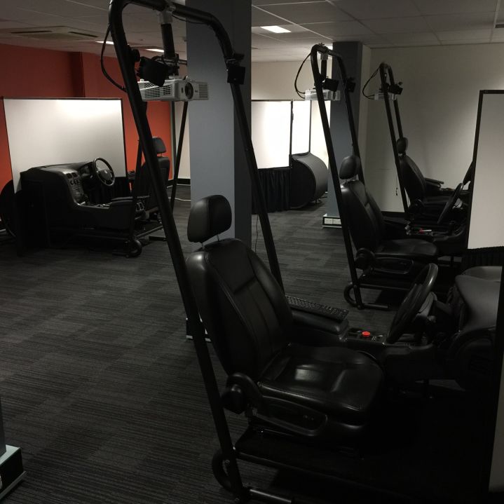
The motorway route was designed to have no intersections or buildings, thereby providing an
experience of driving on a highway, as shown in Figure 5(a). On the other hand, the urban road
alternative replicates characteristics of a usual urban road which consists of a number of buildings,
intersections, and traffic lights, see Figure 5(b). Both routes also have speed signs and other road signs.
Before choices are made in the simulator, each participant is asked to conduct a test drive on both the
motorway and the urban road.
The choices presented in the DSE are exactly the same as the SCE except for the fact that in the DSE,
the participant is faced with simulated experiences of the route travel time, travel cost, and travel
time unreliability after having made a route choice decision.
The benefit of conducting driving simulator experiments (over a more naturalistic experiment) is that
the researcher has a high degree of control over experienced travel times. Travel times in the
simulator are controlled by adjusting the traffic light settings (longer red intervals means longer
delays) and programming computer-controlled vehicles—lead vehicle, tail vehicle, and right-side
vehicle(s). The lead and right-side vehicles ensure that a participant does not start speeding (above
the speed limit) and overtaking, respectively; and the tail vehicle gives a perception of the general
traffic to the participant in the rear-view mirror of the simulator. The scenario is designed in such a
way that when the participant starts driving, the computer-controlled vehicles start driving too (a
sensor is used to achieve this).
9(a) Overview of the TRACSLab@USyd (b) Cockpit of the simulator
Figure 4 Driving simulators at TRACSLab@USyd
(a) Motorway (b) Urban Road
Figure 5 Routes in driving simulator
We did not opt for a long driving segment because (i) our aim of capturing route choice was well
captured in this road segment, (ii) we need to consider multiple drives to reflect multiple choice tasks
in a typical stated choice experiment, and (iii) a long drive in the simulation environment may induce
fatigue earlier than the actual driving and increase the workload, which can compromise data quality.
Therefore, we kept the maximum driving time to 12 mins for a scenario (with regular breaks between
scenarios), allowing us to conduct five choice tasks while ensuring that the workload of the
participants is reasonable and comparable to that in many existing studies using a driving simulator
(Dell’Orco & Marinelli, 2017; Ali et al., 2020b, c). While the individual runs are shorter than what might
be typical in a road safety experiment, the total driving time of each participant in the simulator (plus
potential time savings and cost trade-offs) is representative of a typical trip within Sydney.
103.2.1. Experiencing cost
Each participant receives an initial endowment of $60 and are told during recruitment that their
participation reward will vary on the choices made during the DSE6. To make the payment of the
motorway toll consequential, respondents were shown a jar filled with one-dollar coins as per Figure
6(a), and each time the motorway was chosen, respondents observed two dollars being removed from
the reward jar placed into the “toll revenue” jar. After the experiment, the participant retains any
remaining reward (paid out via a gift card). There is no cost associated with the urban road, so the
reward jar is untouched if this alternative is chosen.
3.2.2. Experiencing travel time and unreliability
Irrespective of the alternative chosen, a participant must experience travel time by driving the chosen
route. However, what is more novel in this experiment is the experience of travel time unreliability.
Suppose again that the participant is faced with the example choice task shown in Figure 3. The
participant is asked to choose their preferred route, fully aware of the travel time distribution of the
urban route (as well as other route characteristics). If the participant chooses the urban route, then
we mimic unreliability by taking a random draw from the known travel time distribution. This is
achieved by showing the participant five cards with travel times that replicate the travel time
distribution (which the participant can verify). Figure 6 (b) shows the five cards used for the travel
time distribution shown in the example choice task in Figure 3. Then the cards were shuffled face
down and the participant was asked to pick a card (without seeing the travel time on the card). A
scenario consistent with the randomly selected travel time was then loaded into the driving simulator
for the participant to experience. It should be noted that:
• After the driving task the chosen card was revealed so that the participant could verify the
experienced travel time. It is important to complete this verification process to maintain trust
between the respondent and the analyst, and in the integrity of the experimental procedure.
• Respondents were clearly informed that the DSE would take a maximum of 90 minutes,
however during the pre-DSE briefing they were told it would be possible to leave the
experiment in a significantly shorter time period depending on the choices made7.
(a) Experiencing cost (b) Experiencing travel time unreliability
Figure 6 Simulated experiences
6
Participants were told the reward would vary between $40 and $60. Furthermore, a respondent received a fee
of $15 if they were not able to complete the study, e.g. due to motion sickness, or if they did not adhere to the
rules regarding speeding and driving off-road in the driving simulator.
7
That is, they can leave early if they finish driving the scenarios earlier if they select Motorway and pay the toll
cost or if they get lucky on the Urban route by drawing a 4 or 6-minute travel time card each time.
114. Experimental Design
We define four levels for toll cost, namely $1, $2, or $3 for the motorway alternative and $0 for the
urban road alternative. Regarding the travel time distributions, the motorway alternative has a fixed
travel time of 6 minutes (which equates to a mean travel time of 6 and a variance of 0) while for the
urban road alternative, we consider combinations of five travel times, where each travel time can be
4, 6, 8, 10, or 12 minutes. These attribute levels were chosen for several reasons, but an important
consideration is that each participant was limited to 90 minutes in the simulator. If a respondent was
unlucky enough to generate 5 choice tasks each with a travel time of 12 minutes, this would require
60 minutes of driving time, with a further 15 minutes of enforced breaks (to avoid simulator sickness).
With other associated time requirements of the experiment, this upper value of 12 minutes per task
was the maximum that could reasonably be expected to be completed within the timeframe given.
With regards to the remaining mix of times and costs, with these attribute levels, if a respondent was
to select only the motorway option in each task, the expected cost across the 5 choice tasks would be
$10, with an approximate time saving of 30 minutes. This would equate to a value of time of
approximately $20 per hour, consistent with the VTT used by New South Wales Government.
In determining the correct design approach, it is imperative to already anticipate the specification of
the econometric model, a point we turn to now. The two route alternatives are described by three
attributes, namely travel (toll) cost, mean travel time, and the standard deviation of travel time
(describing travel time unreliability). Adopting random utility theory in order to describe route choice,
we define the utility of route i for respondent n in choice task t, denoted by U nti , as
U nti = Vnti + e nti . (1)
where Vnti is the systematic utility and e int is a randomly distributed error term. We consider two
routes, and assume that each route is described by a given travel time distribution, denoted by Tnti ,
and given toll costs, Cnti . The systematic route utility is assumed to depend linearly on the average
travel time, standard deviation of travel time, and toll cost. Furthermore, we assume an alternative-
specific constant for the motorway alternative, using a dummy coded variable M i that equals 1 for
the motorway route and 0 for the urban road. Therefore, systematic route utilities are defined as:
Vnti = d M M i + bT E (Tnti ) + b S var(Tnti ) + bC Cnti . (2)
where d M is the alternative-specific constant for motorway and β = ( bT , b S , bC ) is a vector of
marginal utility coefficients.
Eqn. (2) represents a mean-variance model that is often used to account for travel time unreliability.
In the basic model, we assume that the error terms are independently and identically extreme value
type I distributed, which means that route choice probabilities, Pnti , can be computed using a
multinomial logit (MNL) model. That is:
exp (Vnti )
Pnti = . (3)
å i¢
exp (Vnti¢ )
12There exist 3 possible profiles for the motorway alternative, given the fixed travel time and the three
possible toll levels. On the other hand, with five travel times shown for the urban road alternative in
each scenario, drawn from five possible values (4, 6, 8, 10 or 12 minutes), there exist 55 = 3,125
possible profiles for the urban road alternative. However, many of these profiles are essentially
identical, as for example the travel time combination {4,6,6,10,12} represents the same distribution
as {6,12,10,4,6} with the same mean and variance.
Considering only unique travel time distributions, which we represent in increasing travel time order
to participants, there are 126 profiles left for the urban road alternative. Further, we only consider
travel time distributions with a unique mean and variance, e.g. {6,6,10,10,10} has the same mean and
variance as {6,8,8,8,12}, which removes 44 profiles. This means that in total, 246 different choice tasks
exist, which are combinations of motorway and urban road profiles. Choice tasks where the urban
road strictly or weakly dominates the motorway have been removed. For example, a choice task where
the urban road has travel time distribution {4,4,4,4,4} is removed since the urban road strictly
dominates the motorway (as it is cheaper, faster, and has the same reliability). If the urban road has
travel time distribution {4,4,6,6,6} then it does not strictly dominate the motorway according to utility
function (2) because while the urban road is cheaper and faster on average, it is less reliable. However,
we can argue that a distribution of {4,4,6,6,6} is likely preferred over {6,6,6,6,6} despite travel time
being less reliable, therefore we removed such choices tasks with a weakly dominant alternative from
the candidate set. The final candidate set consists of 67 choice tasks.
Not all 67 choice tasks provide the same level of information for estimating the parameters in Eqn.
(1). Given the limited number of participants in driving simulator experiments, we selected a subset
of 15 choice tasks that provide high (Fisher) information for estimating the parameters in our model
in Eqn. (1). This was achieved by generating a D-efficient experimental design through the modified
Federov algorithm in Ngene (ChoiceMetrics, 2018) using our candidate set with 67 choice tasks. This
design minimises the standard errors of the estimated model parameters and thereby minimises the
required sample size (Bliemer et al., 2008; Rose & Bliemer, 2009). For the travel time and travel cost
attributes, we assumed parameter priors based on estimates reported by Bliemer et al. (2017), who
conducted a stated choice survey regarding route choice in Australia. For the standard deviation of
travel time attribute, we assumed a prior consistent with a reliability ratio8 of 0.85 (which is the
average of the range 0.2 to 1.5 as reported in De Jong & Bliemer, 2015). The mean and standard
deviation of travel time were computed for each of the 67 travel time distributions in the candidate
set and once the experimental design was generated, they were converted back to travel time
distributions consisting of five travel times.
Given that each participant could only spend a maximum of 90 minutes in the lab as stated in our
ethics approval, each respondent was asked to complete only five choice tasks. Therefore, we blocked
the design into three blocks of five choice tasks each where we aimed to have some degree of attribute
level balance within each block (e.g. in each block the participant will face each of the toll levels at
least once). The final experimental design is presented in Table 2.
The design of the experiment started in late 2016 and completed by mid-2017. It was followed by
implementing, testing, and conducting pilot studies in the second half of 2017.
8
Reliability ratio (RR) is defined as VOR divided by VTT (or marginal rate of substitution between travel time and
standard deviation of travel time). Assuming a RR of 0.85, the resulting prior for standard deviation of travel
time is equal to -0.122.
135. Sample and Preliminary Results
5.1. Participants
While many DSEs are conducted with students only, we opted to sample from the general population
in order to get more variation in our sample (in particular with respect to age and income). We are
not necessarily concerned with obtaining a representative sample since we are not using the
estimated VTT and VOR for appraisal purposes, but rather are mainly interested in differences in
outcomes between the in SCE and DSE. Unlike SCEs, it is not easy to recruit non-student participants
for the DSEs (despite a reward of up to A$60) since they typically require a larger time commitment
and require the respondent to physically attend the lab.
We used two approaches to recruit participants, using advertisements and contacting participants
from previous experiments conducted at TRACSLab. In advertisements, we adopted a number of
different tools including a University of Sydney (USYD) volunteer database for research studies,
posting study details via USYD Business School official Facebook and Twitter pages and the TRACSLab
website, flyers at the University (including coffee shops), and free local classified ads (via
www.gumtree.com.au).
Table 2 Choice tasks and blocks
Motorway Urban Road
Block Travel times (min) Toll ($) Travel times (min) Toll ($)
* **
6, 6, 6, 6, 6 2 4, 4 ,10, 12, 12 0
6, 6, 6, 6, 6 1 8, 10, 10, 10, 12 0
I 6, 6, 6, 6, 6 1 4, 6, 12, 12, 12 0
6, 6, 6, 6, 6 2 4, 6, 6, 8, 10 0
6, 6, 6, 6, 6 3 8, 10, 12, 12, 12 0
6, 6, 6, 6, 6 1 4, 6, 8, 10, 12 0
6, 6, 6, 6, 6 1 8, 10, 12, 12, 12 0
II 6, 6, 6, 6, 6 1 4, 4, 6, 8, 8 0
6, 6, 6, 6, 6 2 4, 4, 4, 6, 12 0
6, 6, 6, 6, 6 3 4, 6, 10, 12, 12 0
6, 6, 6, 6, 6 1 4, 6, 6, 8, 8 0
6, 6, 6, 6, 6 2 8, 10, 10, 10, 12 0
III 6, 6, 6, 6, 6 1 4, 6, 10, 12, 12 0
6, 6, 6, 6, 6 2 8, 10, 12, 12, 12 0
6, 6, 6, 6, 6 3 4, 6, 12, 12, 12 0
*
6 minutes every day
**
4 minutes two days per week, 10 minutes one day per week, and 12 minutes two days per week.
During the recruitment process, participants complete a screening questionnaire which included
supplementary questions designed to elicit information on their driving experience (i.e., how long they
have been driving), age, sex, income, level of education, and occupation. The participants had to fulfil
the following requirements:
14a) Hold a driving license;
b) Drive at least 10 minutes, two or more days per week;
c) Be at least 18 years old;
d) Not suffer from motion sickness, vertigo, vestibular migraines or epilepsy;
e) Not suffer from any other medical conditions that impact the ability to drive.
The recruitment process was repeated three times in total, with waves in September 2017 to
December 2017; February 2018; and finally November 2018. Although in these three attempts, we
were able to recruit more than 300 participants, only 76 participants actually turned up at the
TRACSLab. With two participants experiencing motion sickness, we retained a final sample of 74
participants. Each participant completed 5 choice tasks in both SCE and DSE, resulting in a total of 740
choice observations. Note that a sample size of 74 participants is high compared to most other driving
simulator studies.
5.2. Descriptive Statistics
The socio-demographic characteristics of the 74 participants that completed the experiment are
presented in Table 3. Comparing our sample to the population of Greater Sydney (ABS, 2016), we do
see an over-representation of respondents who are more highly educated (university degree or
higher), and aged between 30 to 39 years. Respondents in the sample also tend to have relatively
higher incomes.
Table 3 Socio-demographics of the participants
N=74
Characteristics Category
Sample (%) Greater Sydney (%)
Male 44.6 49.3
Gender
Female 55.4 50.7
18-29 28.4 26.9
Age (in years) 30-39 35.1 23.9
40-65 36.5 49.1
49,999 or less 29.7 50.4
50,000-74,999 33.8 16.6
Annual Personal
75,000-99,999 17.6 10.5
Income (A$)
100,000 or more 16.1 13.4
Not answered 2.7 9.2
≥5 44.6 NA
Commuting to work
4 21.6 NA
(days per week)
≤3 33.8 NA
Occupation Employed full-time 46.0 67.9
Employed part-time 54.0 32.1
Year 11 or less 0.0 17.2
High School 13.5 35.5
Education Associate degree (or Trade diploma) 14.9 15.2
University degree or higher 70.2 22.5
Not answered 1.3 9.6
15Regarding the order of experiments, 43 participants completed the two experiments in Order 1 (SCE
first) and 31 participants in Order 2 (DSE first). Figure 7(a) shows the choice share of the motorway
and urban road alternatives by experiment type. With respect to the experiment type, the Motorway
is selected less often in the DSE (26%) compared to the SCE (36%). Therefore, these frequencies
suggest that there may be differences in behaviour depending on the type of experiment.
Figure 7 (b) further displays the choice shares depending on the order in which participants complete
the experiments. We see that in Order 1 (SCE first), the motorway alternative is selected 34% in SCE
compared to 22% in DSE. On the other hand, in Order 2 (DSE first), the motorway alternative is chosen
39% of the time in the SCE compared to 33% in the DSE. These differences in frequencies suggest that
there exists an order effect, which is confirmed by a Chi-Square test ( c 2 (1, N = 74) = 5.66, p < .05 ).
We account for ordering effects in our econometric analysis in Section 5. Note that these figures also
reveal that the choices made in the SCE and the DSE differ to a greater extent in Order 1 than they do
in Order 2.
Figure 7 Observed route choices in SCE and DSE
6. Model Estimation and Results
Given the novel experimental structure and exploratory nature of the work, we adopted a structured
and incremental approach toward estimating models starting with a basic route choice multinomial
logit (MNL) then heteroscedastic logit (HL) models to account for scale differences across the two
experiment types (SCE and DSE experiments) and also order effects, and finally a latent class (LC)
model in order to account for preference heterogeneity across all attributes and the panel nature of
the data (given that we have multiple observations from a single respondent). All models were
16implemented and estimated in R using Apollo (Hess & Palma, 2019). All models are estimated using
pooled data (by combining SCE and DSE data). We excluded two participants from the dataset as they
did not provide their income data, leading to a final sample of 72 respondents.
6.1. Multinomial Logit Model
In MNL 1, as discussed in Section 3.4, we estimate d and β. In MNL2, we investigate whether
preferences for the motorway alternative are different across the two types of experiment, by
estimating an additional shift parameter d MD for the motorway alternative in the DSE (i.e. when
M i = 1 ) which is used when task t for person n is a simulator task (i.e. when Dnt = 1 ):
Vnti = d M M i + d MD M i Dnt + bT E (Tnti ) + b S var(Tnti ) + bC Cnti . (4)
We next tested the inclusion of several sociodemographic variables where we found that only income
had a statistically significant influence on route choice. In order to directly estimate the income
elasticity lI we interact toll cost with a scaled income factor I n for respondent n, where I n is defined
as income divided by average income. This gives us the following utility function for MNL 3:
Vnti = d M M i + d MD M i Dnt + bT E (Tnti ) + b S var(Tnti ) + bC Cnti I nlI . (5)
Table 4 presents parameter estimates for the three MNL models. In all models, we observe that the
estimated parameters for the average travel time, toll cost, and travel time unreliability attributes
have a negative sign, which is expected, and are statistically significant ( p < 0.05 ). In all cases, the
parameter of the motorway dummy is negative, indicating that the (tolled) motorway option is less
attractive than the (untolled but unreliable) urban road option (ceteris paribus). Note that there was
a relatively low negative correlation between the motorway dummy and toll cost (-0.22).
In MNL 2 and MNL 3, we see that the additional DSE shift for the motorway constant is negative and
statistically significant, implying that motorway is disliked more in DSE than SCE. A possible
explanation is that participants are more averse to the tolled motorway (irrespective of the toll level)
when they have to pay actual toll costs in the DSE. We investigate this further in the latent class model
in Section 6.3.
Table 4 Estimation results for MNL models
MNL 1 MNL 2 MNL 3
a
Route attributes
Motorway (d M ) -1.631 (-4.73) -1.381 (-3.77) -1.376 (-3.75)
Motorway x DSE (d MD ) --- -0.543 (-2.49) -0.551 (-2.49)
Avg. travel time ( bT ) -0.512 (-7.30) -0.519 (-7.29) -0.528 (-7.42)
St. dev. of travel time ( b S ) -0.274 (-4.28) -0.278 (-4.29) -0.278 (-4.24)
Toll cost ( bC ) -0.799 (-7.46) -0.812 (-7.44) -0.780 (-6.66)
Income elasticity (lI ) --- --- -0.322 (-2.09)
Model fit
LL (0) -499.07 -499.07 -499.07
LL (final) -397.33 -392.467 -386.963
Adj. Rho sq. 0.196 0.204 0.213
No. of parameters 4 5 6
BIC 820.97 817.83 813.40
a Robust t-ratio values against zero are in brackets.
17In MNL 3, the estimate of lI shows a negative and statistically significant income elasticity towards
toll cost, meaning that the sensitivity towards toll cost decreases with an increase in income. The
relatively low value for the lI may be explained by the fact that we have mostly high income
participants in our sample. The improvements from MNL 1 to MNL 2 (the loglikelihood ratio (LR) test
statistic is equal to 9.72 while c1,95%
2
= 3.84) and then MNL 2 to MNL 3 (the LR test statistic is equal to
11.01 while c1,95% = 3.84) are statistically significant. MNL 3 will serve as the starting point for
2
estimating heteroscedastic models in the next section where we take possible scale differences into
account.
6.2. Heteroscedastic Logit Model
Our data originates from two different sources (SCE and DSE), and there may be different error
variances (i.e. difference in scale) for each experiment type that need to be accounted for. In
heteroscedastic logit (HL) models, we relax the assumption that the error variance is constant within
the data. Furthermore, we also allow for difference in error variances based on order effects, i.e. which
treatment was used first. This thus results in four scale terms in total.
We introduce a dummy variable On that equals 1 if respondent n faces the two experiments in Order
1 (SCE first), and zero in case of Order 2 (DSE first). Applying different scale parameters for each type
of experiment depending on the order leads to the following formulation of the systematic route
utilities:
(
Vnti = µnt d M M i + d MD M i Dnt + bT E (Tnti ) + b S var(Tnti ) + bC Cnti I nlI .) (6)
where we define
ì µ D1 , if Dnt =1 and On = 1 (scale parameter for DSE, when SCE is taken first),
ïµ , if Dnt =0 and On = 1 (scale parameter for SCE, when SCE is taken first),
ï
µnt = í S 1 (7)
ïµD 2 , if Dnt =1 and On = 0 (scale parameter for DSE, when DSE is taken first),
ïî µ S 2 , if Dnt =0 and On = 0 (scale parameter for SCE, when DSE is taken first).
In this model, which we refer to as HL1, we normalise µ D1 = 1 and estimate three scale parameters,
μ = ( µS1 , µ D 2 , µS 2 ). Results are presented in Table 5.
In HL 1 we observe that all estimates for β remain statistically significant (and do so for all subsequent
HL models). Examining the scale terms we note first that µ S 1 is not statistically different from the base
µ D1 = 1. Second, scale parameter µ D 2 is significantly different from the base of µ D1 = 1 , while µ D 2 is
not significantly different from scale parameter µ S 2 (confirmed by testing whether µ D 2 - µ S 2 = 0 ,
where this test incorporated the covariance between the estimates to ensure that the t-ratio on the
difference reflects the maximum likelihood estimate properties of the original parameters; cf. Daly et
al., 2012) and scale parameter µ S 2 is significantly different from 1 at the 10% level. Our findings thus
suggest that scale differences exist by order but not by experiment type (SCE vs DSE).
Given the above results, a second model (HL 2) was estimated that only includes scale differences due
to experiment order, such that the systematic route utilities simplify to:
( )
Vnti = µ21-On d M M i + d MD M i Dnt + bT E (Tnti ) + b S var(Tnti ) + bC Cnti I nbI , (8)
18where we estimate scale parameter µ 2 corresponding to Order 2 (DSE first, On = 0 ) while scale is
equal to 1 for Order 2 ( On = 1 ). Parameter estimates shown in Table 5 suggest a lower scale
parameter, and hence more error variance, for data collected using Order 2. One possible explanation
for this result is that those respondents who complete the DSE first may exhibit more variety seeking
behaviour and try out both routes in the simulator, e.g. participants are likely to sample the Motorway
a number of times, or they are still learning about the nature of the experiment. Then, when
completing the SCE two weeks later, they may make similarly stochastic choices in the context of the
absence of consequence to the choices made.
On the other hand, another possible explanation is that, in Order 1 (SCE first), participants may be
observed to make relatively more consistent choices because all information is presented in the SCE
to participants and no travel time, travel time unreliability, or toll costs are experienced. When
confronted with the DSE that now includes experience/experimental consequence, respondents are
more incentivised to reveal their preferences towards these attributes and/or have learnt the nature
of the experiment from the SCE and thus are less prone to variety seeking in the DSE.
While identifying one unique explanation for the result is not possible, a clear order effect can be
observed via the impact on scale. Overall, we prefer HL 2 over HL 1 because model HL 2 is more
parsimonious than HL 1 (the LR test statistic is equal to 0.71 whereas c 2,95%
2
= 5.99).
Building on model HL 2, we further explored preference heterogeneity towards route attributes in the
two experiment types by estimating multipliers in the case of DSE, which leads to the following utility
functions for model HL 3:
( )
Vnti = µ21-On d M M i + d MD M i Dnt + kTDnt bT E (Tnti ) + k SDnt b S var(Tnti ) + k CDnt bC Cnti I nbI . (9)
where we estimate preference parameters β, scale parameter µ 2 and attribute-specific multipliers
κ = (kT , k S , k C ), which only apply in case of the driving simulator experiment where Dnt = 1. Table 5
presents parameters for HL 3, where we clearly observe that none of the multipliers are statistically
different from 1. Initially, we expected that participants would be more sensitive to time and cost
attributes in the DSE because they had to experience them. However, from HL 3 we cannot draw this
conclusion. HL 3 also does not improve model fit over HL 2 (the LR test statistic is equal to 1.02 whereas
c 3,95%
2
= 7.81).
6.3. Latent Class Model
To further explore potential differences in preferences, we estimate a latent class (LC) model with two
classes, qÎ{1,2}, with the following class-specific systematic utility functions:
(
Vnti|q = µ21-On d M M i + d MDq M i Dnt + kTDnt bTq E (Tnti ) + k SDnt b Sq var(Tnti ) + k Cq
Dnt
bC Cnti I nlI .) (10)
and for the class assignment model, we simply use utility function Vq = a q , where we normalise
a 2 = 0 and estimate only a constant for Class 1. We tried including sociodemographic variables in the
class assignment utility function, but none were found to be statistically significant. We estimate class-
specific preference parameters d MDq and β q while we keep d M and lI generic across both classes
since making them class-specific did not significantly improve the model fit. Also, attribute-specific
multipliers κ are not considered class-specific to ensure that the model parameters are identifiable.
We tried increasing the number of latent classes but a model with two latent classes was preferred
based on the Bayesian Information Criterion (BIC), and consideration was also given to the application
of the model and the practicability of the results (Beck et al., 2013).
19You can also read