ANALYSING THE EFFECTS OF WEATHER TO REGIONAL BUS TRAFFIC IN TAMPERE REGION - Faculty of Information Technology and Communication Sciences M. Sc ...
←
→
Page content transcription
If your browser does not render page correctly, please read the page content below
Konsta Peltola

      ANALYSING THE EFFECTS OF
WEATHER TO REGIONAL BUS TRAFFIC
              IN TAMPERE REGION

   Faculty of Information Technology and Communication Sciences
                                                  M. Sc. Thesis
                                                      April 2019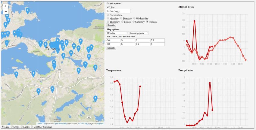
ABSTRACT
Konsta Peltola: Analysing the effects of weather to regional bus traffic in Tampere region
M. Sc. Thesis
Tampere University
MDP in Software Development
April 2019

The topic of this thesis is to study how weather is affecting regional bus traffic in Tampere
region. Study focuses on evaluating the direct effects of air temperature and snowfall. Delays of
regional bus traffic were evaluated by using real time location data and timetable schedule data
from regional buses in Tampere region. Based on this information, link travel times were
counted for each stop-to-stop trip on the route of the bus. This approach also enabled the
evaluation of between which stops the biggest delays occur and during which time of the day.
The weather conditions were evaluated by using open weather observation data from Finnish
Meteorological Institute and different ranges of air temperature and precipitation were
categorized. Link travel times during good driving conditions were used as a baseline when
compared to link travel times observed during more challenging conditions. Effect of weather
was also evaluated during different times of the day and week.

It is expected that there is a correlation between adverse weather and longer link travel times in
bus traffic.

    • Hypothesis 1a: Adverse weather causes longer link travel times for the bus traffic

    • Hypothesis 1b: Effects of adverse weather to link travel times are more severe in specific
         stop-to-stop links

First objective is to evaluate Hypothesis 1a and to find out how clear and big the correlation
between severe weather and changes in bus link travel times are. Objective of the study is also
to try to find out which components of the weather are affecting the link travel times more (air
temperature or precipitation).

If hypothesis 1a is proven to be true, the next object will be to try to examine if delays are
affected by weather more in some specific places or areas of the region.

Key words and terms: weather, congestion, probe vehicle network.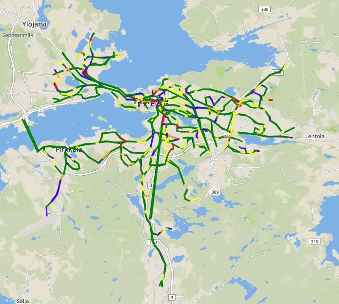
iii

Contents
Contents ...........................................................................................................................iii
1. Introduction ............................................................................................................... 1
2. Measuring road traffic ............................................................................................... 2
   2.1. Automated traffic sensor networks .................................................................. 3
            2.1.1. Fixed sensors ........................................................................................ 3
            2.1.2. Mobile sensing ..................................................................................... 4
            2.1.3. Vehicular sensors ................................................................................. 5
   2.2. Buses as probe vehicle network ....................................................................... 6
3.    Previous work discussing the effects of weather to traffic ........................................ 8
      3.1. Effects in urban areas ....................................................................................... 9
      3.2. Effects in non-urban areas .............................................................................. 10
      3.3. Evaluating the results of previous work ......................................................... 12
      3.4. Indirect effects of weather .............................................................................. 14
4.    Data sources used in this study ................................................................................ 15
      4.1. Bus data .......................................................................................................... 15
            4.1.1. Tampere public transport SIRI interface ............................................ 16
            4.1.2. General transit feed specification (GTFS).......................................... 17
            4.1.3. Journeys API ...................................................................................... 18
      4.2. Weather data .................................................................................................. 20
      4.3. Map data ......................................................................................................... 21
5.    Technologies used in this study ............................................................................... 22
      5.1. Data collection and pre-processing ................................................................ 22
      5.2. Database ......................................................................................................... 22
      5.3. Data processing .............................................................................................. 22
      5.4. Data presentation............................................................................................ 23
6.    Data collection and analysation system ................................................................... 23
      6.1. Data collection and pre-processing ................................................................ 23
            6.1.1. Bus data .............................................................................................. 24
            6.1.2. Weather data ....................................................................................... 27
      6.2. Database structure .......................................................................................... 28
      6.3. Data processing and presentation ................................................................... 29
7.    Results ..................................................................................................................... 31
      7.1. Identifying the recurrent delays during different times of the day on different
      days of the week ...................................................................................................... 32
      7.2. Identifying the weather categories ................................................................. 35
      7.3. Overall effects of air temperature to link travel times ................................... 37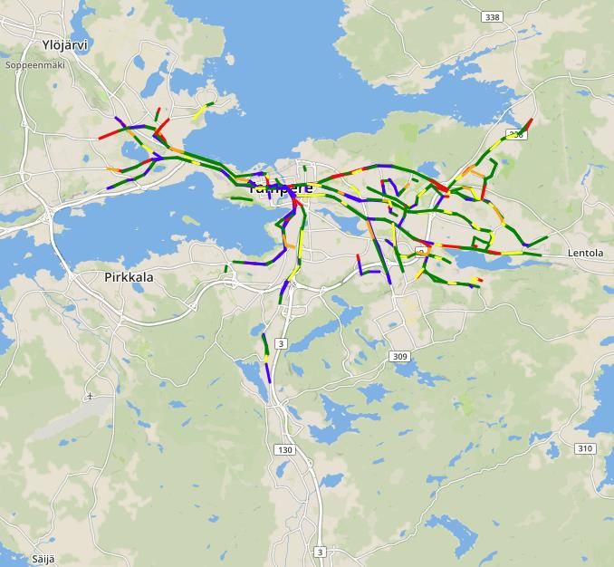
iv

      7.4. Overall effects of snowfall to link travel times .............................................. 39
    7.5. Links where the effects of snowfall to link travel times are the biggest ........ 41
8. Conclusions ............................................................................................................. 45
References ...................................................................................................................... 46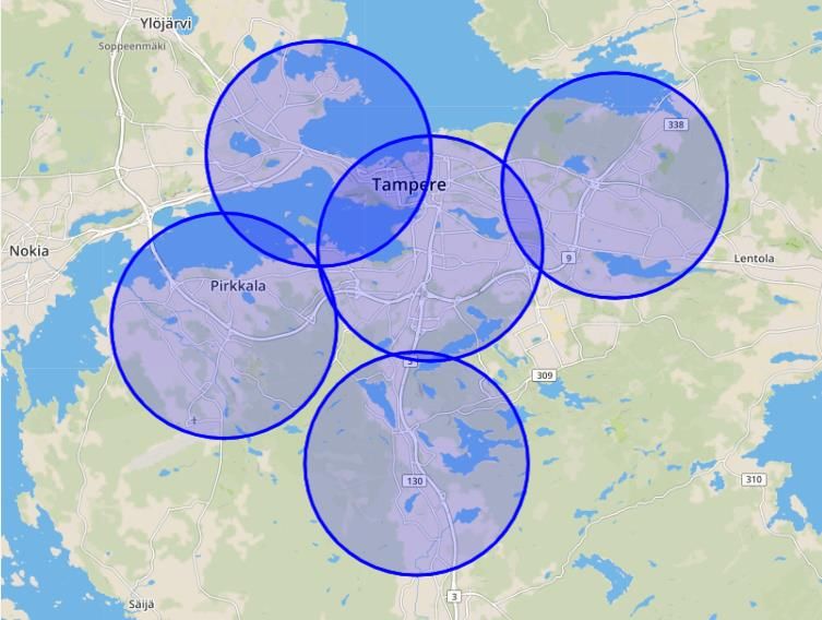
1

1. Introduction
The ever-increasing amount of traffic and resulting congestion in cities have large social
and economic impacts in modern world. Lots of valuable time and fuel is wasted while
people are standing in traffic jams and predicting of traveling times is harder. Therefore,
congestion causes stress for the commuters, increases air pollution and increases the
wear and tear of vehicles. The ways to tackle the issues are either to increase the
capacity of the traffic system, decrease the amount of traffic, or to make the traffic flow
more efficient on the existing traffic network. Increasing the traffic system capacity,
especially in cities, is expensive and transportation infrastructure often takes up a lot of
the space that otherwise could be used for something else. So as a result, there is a great
need for solving the congestions issues by reducing the demand and by using the
existing traffic system more efficiently.
    This is where the public transportation and modern intelligent traffic systems (ITS)
step in. Public transportation increases the amount of people that can be moved through
the traffic system. It is easy to understand that 30 people and their private cars take up
much more room on the streets and on the parking lots than 30 people travelling with a
regional bus or with a tram. Intelligent traffic systems can both increase the throughput
of the traffic network and encourage people to use correct forms of public transportation
on correct time of the day, depending on their destination. As we know, most of the
issues with traffic systems come up during the rush hours so one of the best solutions to
traffic congestion is to try to make rush hour peaks less steep. Additionally, if the
passenger information systems, which are part of the intelligent traffic system, succeed
in making the travel of passengers in public transportation easy and fast, passengers are
much more likely to use the public transport also in the future. [Bacon et al., 2011]
     During recent years, the increasing worry about the climate warming has also
become one of the key factors why we should improve our public transportation systems
and encourage people to use the services of public transportation more. The key factor
in achieving this goal is to develop more intelligent traffic systems which encourage
people to make the more ecological decision of using public transportation instead of
commuting with their private cars.
    The most common effects of congestion are experienced during recurrent delays
caused by rush hour traffic, but weather is known to be one of the reasons which might
cause non-recurrent congestion and issues in the traffic network. Research by Shrank
and Lomax [2001] suggests that adverse weather causes 27% of all non-recurrent traffic
congestion and according to the Highway Capacity Manual [Transportation Research
Board, 2000], rainfall reduces speeds on highways by 2 – 17% and snowfall by 3 – 35%
depending on the intensity of precipitation.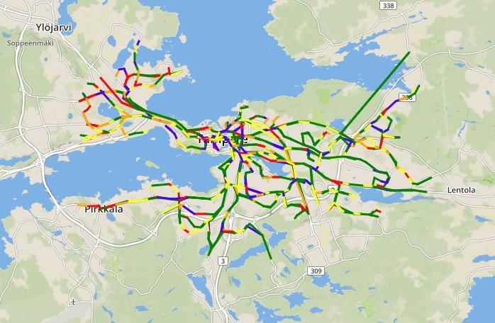
2

    The effect of weather can be direct, by making people drive more slowly, or
indirect, e.g. by people choosing different means of transportation or by increasing the
amount of accidents which can then cause even more congestion. According to Andrey
et al. [2001], precipitation increases the risk of accidents from 50 to 100 percent. The
direct effect of weather to delays in regional bus traffic is what this study is focusing on
trying to evaluate. This objective is pursued by recording bus link travel times between
consecutive bus stops from live location data provided from Tampere regional buses
during different weather circumstances. By comparing the link travel times during
different weather circumstances, it is also possible to evaluate if delays occur more
often in some specific areas of the road network. Link travel times are also recorded
based on the day of the week and time of day. This enables also the evaluation of the
day of the week or time of day when the biggest delays occur.
    Paula Syrjärinne made her doctoral thesis in 2016 about analysis of traffic data from
buses in Tampere region. During the writing of her thesis, Syrjärinne acted also as a
supervisor for my bachelor’s thesis. This is one of the reasons why I also became
interested in the topic of bus location data. Combining bus travel time data and weather
data was one of the suggestions for future research topics by Syrjärinne. Therefore, her
doctoral thesis and its results are in multiple occasions acting as a base for this study.
    Next, in Chapter 2 I explain the basics and scientific background of how traffic can
be measured and monitored. After that, in Chapter 3 I review the previous scientific
work which has been examining the relation between weather circumstances and road
traffic. In Chapter 4 I describe the sources of bus location and weather observation data
which were used in this study. Chapter 5 gives an overview of the software
development technologies used in this study. Chapter 6 focuses on describing the
automated data collection and analysation system which was developed during this
study. In Chapter 7 I present the results of the study and finally in Chapter 8 I evaluate
the overall success and value of the study.

2. Measuring road traffic
There are multiple ways of measuring traffic amounts and fluency and each of these
ways has its strengths and weaknesses. The oldest way, which is still being used today,
is by using manual calculations from personnel counting traffic amounts on the ground
[Toth et al., 2013]. This is of course quite an accurate way of counting the traffic
amounts and gives also the possibility of counting many different types of traffic, for
example pedestrians and cyclists, but there is a possibility for human error in the
counting. Also, it is easy to understand that in order to get 24/7 real-time information
about the status of the traffic in the entire city or area, automated sensors and systems
have to be developed instead of relying on manual counting.
3

2.1. Automated traffic sensor networks
Today, there are multiple different technologies which can be used to automatically
measure traffic. Biggest difference comes from the placement of the measurement
devices, as they can be fixed and installed to the road infrastructure (e.g. on the side of
the road), they can be placed onboard the vehicle itself or they can be carried by
passengers who are using the traffic network. Next, I will explain some of the most
common systems in more detail.

2.1.1. Fixed sensors
Traditionally automated traffic sensor systems have been based on fixed sensors. Today
there are multiple different kinds of fixed sensors which are using different technologies
to measure the traffic.
      Most common type of fixed sensors are inductive loops which are installed to the
road pavement. Single inductive loop can only detect presence and size of a car on one
lane from the change the car makes to the electro-magnetic field of the loop. However,
when this kind of loops are installed as a pair, it is possible to determine also the
direction and speed of the vehicle. However, it is not possible to identify a specific
vehicle from a group of vehicles with a loop detector, so for example counting of link
travel times for a specific vehicle is not possible with loop detectors. In Finland,
inductive loops are the common way to detect if there is a vehicle approaching or
already waiting in the intersection. Often information about different intersections is
also combined so traffic lights in different intersections work in cooperation with each
other to improve the performance of the traffic system. Inductive loops are quite
expensive to install and difficult to maintain, as repairs can’t be made without
disrupting the traffic. Also, inductive loops might not detect motorcycles as their
magnetic mass is much smaller. In addition to usage of inductive loops to detect
vehicles in traffic light controlled intersections, loop detectors are often used in
monitoring traffic speeds and volumes on freeways. Also, some implementations of
automatic traffic and speed monitoring by the police can be based on inductive loops.
[Bacon et al., 2011]
      One alternative for inductive loops is detecting traffic volumes from traffic
cameras. With a single camera, it is possible to detect speed and direction of vehicles
from multiple lanes [Bacon et al., 2011]. Camera can also detect the size of the vehicle
and with multiple cameras and automatic number plate recognition system it is also
possible to count travel times for individual vehicles between two points in the traffic
system [Tsapakis et al., 2013]. Camera based systems are easier to maintain than
inductive loops, but they are more vulnerable for external circumstances e.g. snow
blocking the lens.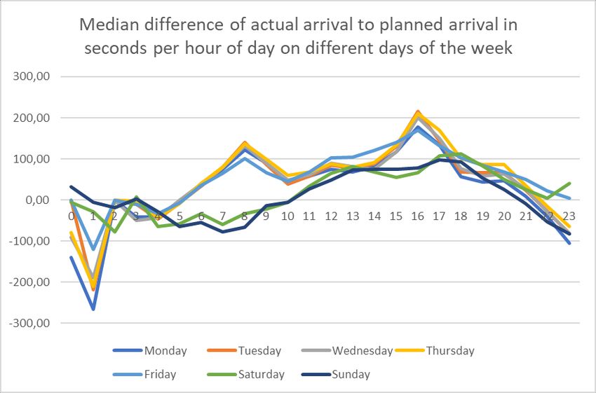
4

      Another commonly used type of fixed sensor is Remote Traffic Microwave
Sensor (RTMS). RTMS sensors are mounted on the side of the road and therefore also
easier to install and maintain without disrupting the traffic than loop detectors. A RTMS
sensor is transmitting microwave beams towards the road and can detect movement
from the beams which are reflected back to the sensor from objects within the target
area. This enables the RTMS sensor to monitor traffic volume, occupancy and speeds
from multiple lanes at the same time. According to study by Yu and Prevedouros [2013]
the speed measurement accuracy of RTMS can be up to 95% and therefore is higher
than the accuracy of a single loop detector. [Ma et al. 2015]
      All types of fixed traffic sensors have some limitations in the information they can
provide. As the name already says, the sensors are fixed and therefore can provide
information only from the roads where sensors have been installed. Sensors of this kind
are quite expensive to install and therefore the coverage of the sensor network is not
often very extensive. The high price is also the reason why fixed sensors are more often
used for monitoring of highway traffic instead of traffic flow on urban areas.
      For example in Finland, Finnish Transport Agency has about 500 active fixed
automatic traffic measuring stations, also known as LAM (Liikenteen Automattinen
Mittausasema) -stations. The LAM -station consists of two inductive loops installed to a
single road lane. With this setup, it is possible to detect the direction, speed and
length/size of the vehicle. Most of the sensors are placed on highways and the
information from LAM stations is open to public but wasn’t used in this study. [Finnish
Transport Agency, 2018]
    The inductive loop sensor data from some of the intersections in Tampere region is
also available to the public. From this information it is possible to get the traffic
volumes and length of the queues on intersections at a given time. However, data from
these sensors wasn’t used in this study, as it doesn’t give information about the effects
of weather to travel times. [ITS factory, 2018]

2.1.2. Mobile sensing
Mobile devices that are carried by the passengers themselves can also be used as data
sources for traffic monitoring. Different levels of mobile sensing have been identified,
based on the involvement of the person carrying the mobile device. Some systems
require manual input from the passenger, some require special device or on smartphone
special permissions or software to be installed on the device and some systems might
work even without the user of the device necessarily knowing about it.
    This kind of mobile sensing is usually based on the GPS/GNSS receivers of the
passenger’s mobile device. However, some systems might also use accelerometers or
WLAN or cellular radios of the device to better determine the location of the device.
[Syrjärinne, 2016]
5
Good example of an application that uses also manual input from the users is
mobile application called Waze. The user selects the address where he or she wants to
drive to and the application will suggest the fastest route based on traffic status data
provided by other users of the application. Some of the data, e.g. driving time and route,
is reported automatically, but the user can also manually add information about road
incidents, e.g. an accident, or even police speed traps, so other users can avoid using the
affected route. [Waze, 2019]
Good example of an application that can collect data even without the average user
even knowing about it is Google Maps, as traffic status information shown in Google
Maps is based on data from mobile sensors (usually smartphones) carried by the
passengers. This kind of data collection is called crowdsensing. Many of the people who
carry their smartphones might not even know that they are sharing their location data to
instances like Google. Therefore, the justification of this kind of data collection has
often been questioned. However, the data which is available by crowdsensing gives
much more detailed and extensive data regarding the status of the road network when
compared to other types of traffic sensor networks. [Bacon et al., 2011]
Mobile sensing is in many ways better for monitoring of traffic in urban areas than
fixed sensors. Mobile sensing is relatively new and cheap way of measuring traffic as
nowadays most people are carrying smartphones with them wherever they go.
However, there are still some open questions regarding the privacy of location data
which is being collected from personal devices of passengers without them necessarily
knowing about it.
2.1.3. Vehicular sensors
Real time location data can also be collected from wireless devices which are installed
directly to the vehicles. Today most of new cars contain devices of this kind already
from the factory, but usually the location information collected from these devices is not
available to the public, the infrastructure or to other vehicles. The vision for the future is
that the vehicles and the infrastructure could communicate with each other, in a
standardized manner, to find the most efficient ways to direct traffic through the entire
traffic network as fluently as possible [Parrando and Donoso, 2015].
As the data from sensors which are installed to cars on the factory is not available,
separate wireless real-time location devices have been installed to vehicles to detect and
report the status and location of the vehicle in traffic network. Often devices of this kind
are installed to cars owned by companies, e.g. buses, taxis, ambulances and delivery
vehicles. Therefore, these location transmitting devices are usually developed for
different use cases than monitoring of the traffic flow. Vehicles which have been
equipped with real time location devices are usually called probe vehicles or floating
cars and together they are called a probe vehicle fleet. Most common use cases for
vehicular sensors are e.g. if the vehicle gets stolen or taxi driver sends an emergency6
signal and therefore the update frequency of location data is often fairly low (e.g. once
per minute). Some studies have tried to tackle the issue of using low frequency location
data for traffic monitoring by developing models to estimate travel times for links also
when distance between location pings is longer than the travel link itself [Jenelius and
Koutsopoulos, 2013]. Data which has been collected from different kinds of probe
vehicles also have their own characteristics which need to be considered when analysing
the data. For example, taxis and buses often have special lanes is cities, so location data
gathered from these vehicles might not actually tell the whole story about status of
traffic for private vehicles. Therefore, it is important to evaluate the assumptions about
what can actually be evaluated based on the data that has been gathered from the probe
vehicle fleet.
For different uses cases of the data which has been gathered from vehicular sensors,
different meta data would also improve the usability of the data. For example, for traffic
flow research it would be good to not only know the location of the vehicle but also
how many people there are onboard. This would enable for example the studying of
which bus stops are most popular during which times of the day. Many buses have this
kind of passenger counting systems installed but at least from Tampere, the passenger
counting information is not available to the public. Also, to be able to detect the arrivals
and departures to bus stops from bus location data more precisely, data from the
opening and closing of the bus’s doors would be useful.
There have been studies about using taxi fleet as a probe vehicle network but data
from taxis has its own specialities. Taxis are moving freely around the road network and
they are not following predefined routes or schedules. This makes the coverage of probe
vehicle data recorded from taxis very extensive but harder to analyse, for example when
compared to data collected from bus fleet. Often the biggest issue with location data
collected from taxis has been the low frequency of data. Also, if it is not possible to see
from the data during which times the taxi had a customer, it is not easy to detect only
from the location data of the taxi whether it is waiting for a customer or standing in a
traffic jam with customer onboard. [Kuhns et al., 2011] [Jenelius and Koutsopoulos,
2013]
There have been lot of studies where regional buses have been fitted with devices
which are sending real time location data. This kind of location data has also been used
in this study and therefore the usage of buses as probe vehicles has been discussed in
more detail in chapter 2.2
2.2. Buses as probe vehicle network
Buses as probe vehicles also have their own characteristics. They are following a
predefined route and a schedule, and this makes it easy to observe if bus is running late
from schedule. On the other hand, because buses are following a route, probe vehicle
data from buses might not cover as much of the road network as data from taxis or7
private cars could. Also, some metadata is needed in order to know which bus is
running on which route.
Syrjärinne [2016] has already studied real time bus location data from same real-
time interface which was used in this study. Based on the location data, she monitored
the performance of the public transport and the traffic fluency in overall.
To detect the combination of time, location and bus line which are regularly
associated with delays, Syrjärinne applied frequent item set mining to the bus location
data. Based on this information a concept of adaptive, data driven bus schedules was
introduced which are taking these recurring delays into account when presenting the bus
departure times to the user. With this system, the user can download the data driven bus
schedule for a bus stop of his or her choice. Data driven bus schedule presents the
forecasted departure time of each bus which is leaving from the selected bus stop, based
on the historical data from recurring delays. User is also informed with an estimated
accuracy of the forecast based on the variance of the historical data. [Ajoissa pysäkillä,
2015]
Regarding the performance of public transportation, Syrjärinne also examined the
effects of traffic light prioritisation for buses which were running late from schedule.
The prioritisation system can detect if a bus which is running late from schedule is
approaching the intersection and can change the sequence of traffic lights so that the bus
doesn’t have to wait for the traffic lights to change for as long as it would without the
prioritisation. Syrjärinne had recorded bus location data both before and after the traffic
light prioritisation system was taken into use in Tampere. The result was that in most of
the intersections the effect of prioritisation system was positive. This means that buses
which were running late, could better catch up their schedule between the stops.
Syrjärinne also studied how bus location data could be used to monitor overall
traffic fluency in the city. For this purpose, she presented the concept of link travel
times, which was also used in this study to find the differences in travel times during
different weather conditions. In her study, history data of link travel times was used to
generate link travel time profiles. From these profiles it was possible to identify the
regular delays associated with specific bus lines. Syrjärinne used these link travel time
profiles to create a real time incident detection system. By comparing the link travel
time profiles and real time location data, the system was able to detect abnormal and
significant delays and report them in few minutes after an incident had happened.
[Syrjärinne, 2016]
Uno et al. [2009] used bus probe data to evaluation of travel time variability and
the level of service of roads. For travel time variability study, they used bus probe data
from Hirakata city, Japan. Bus location data wasn’t provided in real time but instead it
could be uploaded from onboard system of the bus every time when the bus returned
from service back to the depot. Therefore, as the frequency of the location data was not8
limited by the bandwidth of mobile data connection, the frequency of the location data
was good (1 second). As there was no metadata attached to the location data, they also
had to create a supplemental survey for an investigator who then recorded the positions
of the bus stops along the route. They also recorded the travel times for same routes
with a private car. After subtracting the time spent on bus stops from the travel times of
the bus, their result was that the travel time of the bus was nearly the same as the travel
time with a private car.
For the level of service study, Uno et al. [2009] evaluated two things: The average
travel time spent on distance of 1 kilometre and the variation of the total travel time of
the route. On the area, from which they had collected their bus probe data from, new
highways were opened in 2003. This enabled them to compare the results from 2002
and 2003 to see whether the opening of the new highways might have affected the
performance of the traffic network. Their result was that the average travel time for 1
kilometre was shorter in 2003 than in 2002 and also the variance of travel times had
decreased. So, in overall, they concluded that most probably this improvement in the
level of service of the road network was due to the opening of the new highways.
Location data from buses has even been used to detect the cycles of fixed time
traffic signals. Fayazi et al. [2015] studied low frequency bus location data in San
Francisco, USA, to estimate the cycles in which the city’s fixed traffic lights operate.
Their study was successful, and this kind of information can be used for example to
improve fuel efficiency by telling the bus driver to slow down for red lights even before
the light has changed from green.
3. Previous work discussing the effects of weather to traffic
There are a lot of earlier studies regarding the non-recurring effects of adverse weather
to the traffic performance. These studies can roughly be divided into two categories:
Effects of weather in urban areas and effects of weather in non-urban areas. First, I will
examine the effects of adverse weather in urban areas on Chapter 3.1 and then I will
examine the effects of adverse weather on more remote areas on Chapter 3.2. The
results from research that are easily comparable are examined in Chapter 3.3. I have
also shortly examined the previous work regarding the indirect effects of weather to
traffic in Chapter 3.4.
Many of the previous studies are more concerned about the maximum traffic flow
during different weather circumstances because they are focused on trying to understand
the weather-based congestion. Traffic flow means the number of vehicles passing a
certain point in the traffic network for example per hour. However, as my study is
focusing more on understanding the differences in travel times during different weather
circumstances, I have focused on gathering the results regarding the changes in speed,
travel time and other variables which are more relevant to this study.9
There have also been previous studies regarding the effects of darkness and daylight
to traffic, but as the results have been varying and as the counting of this effect is more
complex when the length of the day was changing rapidly during the data collection
period, this effect hasn’t been taken into account in the results of this study.
[Transportation Research Board, 2000] [Jägerbrand and Sjöbergh, 2016]
3.1. Effects in urban areas
Tsapakis et al. [2013] studied the effects of rain, snow and air temperature to travel
times in the Greater London area by using fixed, camera-based sensors and automatic
number plate recognition. They gathered traffic data from three 2-hour periods on
weekdays during the morning, afternoon and the evening. Weather data was available
from multiple weather stations once per hour. First part of their research was to find out
how big radius they could use from weather stations to reliably estimate the amount of
precipitation on the road from which they are measuring the travel times. By comparing
differences in precipitation amounts between different weather stations, they decided to
use a value of 3 kilometres as the radius. This means that only travel links within this
radius from nearest weather station were considered as valid for the examination. Result
of their research was that the temperature had little or no effect in the travel times. The
effect of rain was somewhat related to the amount of rainfall as light rain caused delays
from 0.1% to 2.1%, moderate rain delays from 1.5% to 3.8% and heavy rain delays
from 4.0% to 6.0%. The effect of snow was also greatly dependent on the amount of
snowfall as delay caused by light snow was from 5.5% to 7.6% and by heavy snow from
7.4% up to 11.4%. Tsapakis et al. [2013] also noted that the magnitude of the effect to
travel times was smaller in the central London and inner London area than in the outer
London area.
Xu et al. [2013] examined effects of weather to road network performance in
Haizhu district, China. Traffic data was gathered from more than 20,000 taxis with
location data sampling rate between 20 and 120 seconds. Additionally, data from fixed
sensors in some of the intersections on the selected routes was used. For measurement
of weather, they used only one weather station located near the Sun Yat-Sen university.
However, the longest distance from the weather station to the road being monitored was
only about 2 kilometres. To get comparable results for rainy and non-rainy situations,
they recorded data as a set of rainy and non-rainy days from the same day of the week
and with maximum difference of two weeks between the two dates. They got clear
results that precipitation decreased the performance of the road network. Additionally,
they noted that in their research the effect was more significant during the evening rush
hour than during the morning.
Smith et al. [2004] studied the impact of different intensities of rainfall to urban
freeway traffic capacity and operating speeds in Virginia, United States. Traffic data
was collected from two urban freeway links with 2 -minute intervals. These two10
freeway links were selected for investigation because they both were within 4,8
kilometre (3 mile) radius from the weather station which was used for the study.
Weather station was located at the Norfolk International Airport and precipitation data
was available on an hourly basis. Weather and traffic data from August 1999 to July
2000 was used in the study. One of the main goals of the study was to set exact values
for categorizing of light and heavy rainfall as this wasn’t always clearly stated in earlier
studies which they had examined. Their result for the categorisation was that rainfall
was considered light when precipitation was between 0,254 and 6,35 millimetres per
hour and heavy when rainfall was more than 6,35 millimetres per hour. Results
regarding the effects of rainfall to operating speeds was that light rain caused average
operating speed decreases from 4,84% to 6,11% and heavy rain caused operating speed
decreases from 5,43% to 6,41%.
3.2. Effects in non-urban areas
Chung [2012] examined effects of rain and snowfall to traffic volumes and speeds on
freeways in Korea, based on data from year 2008. According to his results, the effect of
rainfall was clearly affected by its intensity. He also concluded that during the whole
year, rainfall of less than 1 millimetre per hour caused an average of 1071 vehicle hours
of non-recurrent congestion per freeway kilometre while rainfall of more than 30
millimetres per hour caused an average of 2282 vehicle hours of non-recurrent
congestion per freeway kilometre. He also noticed that the effect of rainfall to non-
recurrent congestion was biggest during the afternoon peak hours (16:30 – 20:00) and
smallest during the night (20:00 – 07:00). Chung applied the same logic into studying of
the effects of snowfall to traffic volumes and speeds. The effect of snowfall during
different times of the day was nearly the same as with rainfall but the effect to average
vehicle hours of non-recurrent congestion per kilometre was bit different with snowfall.
The average non-recurrent congestion was rising only until the amount of snowfall
exceeded 25 millimetres per hour. After that the average non-recurrent congestion per
kilometre started to decrease. According to Chung, this was most likely due to reduced
traffic demand and suggest that people will start to avoid travelling once the snowfall
gets so heavy. The amounts of precipitation observed by Chung are very extreme when
compared to precipitation amount observed in this study.
Ibrahim and Hall [1994] studied the effects of adverse weather to freeway traffic
in Mississauga, Ontario. Traffic data was collected from two double loop detectors with
30 second frequency and weather observations were retrieved from weather station
located in Pearson International Airport. To get more data including both rainfall and
snow, data from October, November and December 1990 and January and February
1991 were selected. When analysing the traffic data on clear, rainy and snowy days,
Ibrahim and Hall noticed that the differences between days with similar weather
conditions were smaller during clear weather conditions than during rainy and snowy11
conditions. Therefore, they decided to use data from days with clear weather as one base
dataset and compare that to different rainy and snowy days to get the minimum and
maximum effects of rainfall and snowfall. Their result was that during the maximum
observed traffic flow, heavy rain caused speed decrease of 10% and heavy snow
decrease of 45% in traffic speeds.
Kyte et al. [2001] investigated the effects of adverse weather conditions to free-
flow speeds on rural Interstate freeways in south-east Idaho. Free-flow speed is defined
as the mean speed of passenger cars in low to moderate traffic volumes in prevailing
traffic conditions. As a difference to previous studies, they examined also the effects of
fog and high winds in addition to wet and snowy pavement. Another special feature of
this study is that the data has been gathered from a relatively long period of time
compared to other studies as it was collected from 1996 to 2000. Their results suggest
that reduced visibility has only minor effect to passenger vehicle speeds until the
visibility decreases to less than 300 meters. After this point, the speeds start decreasing
significantly. The decreasing of visibility can be caused for example by fog, heavy
rainfall or heavy snowfall. According to their results, also high winds seem to start
affecting the passenger vehicle speeds after wind speed exceeds 6,7 meters per second.
However, high winds also seem to increase the variance of passenger vehicle speeds
which could be explained by gusty wind, different types of vehicles reacting differently
to wind or different drivers reacting differently to high wind conditions. Regarding the
effects of wet or snowy pavement, their result was that wet pavement reduced the free-
flow speeds by 9,5 kilometres per hour and snowy pavement reduced free-flow speeds
by 16,4 kilometres per hour.
Chin et al. [2004] estimated the yearly weather-related capacity reductions and
weather-related delays in the entire USA based on data from 1999. They used estimates
for reduction of capacity and speed based on previous studies. During light rain, they
estimated that speed reduction would be 10% on all types of roads. During heavy rain,
speed reduction was estimated to be between 10% and 25% based on the type of the
road. Light snowfall was estimated to reduce speeds by 15% on freeways and 13% on
smaller, arterial roads. For heavy snow, speed reduction was estimated to be 38% on
freeways and 25% on arterial roads. The result of the estimation was that during the
whole year, all weather-related events caused capacity reduction of 20,9 billion vehicles
on freeways and principal arterial roads. This reduction in capacity was estimated to
have caused 330,1 million vehicle-hours of delays. If these estimates are even remotely
correct, it is easy to understand why it is important to try to better understand the effects
of adverse weather to traffic performance as so much more time is spent in traffic due to
adverse weather.12
3.3. Evaluating the results of previous work
As is easily noticeable from previous chapters, there have been much more studies
investigating the effects of weather to traffic in freeway settings than in the urban traffic
network. This is because most of the studies are based on traffic data from fixed
sensors, like loop detectors, which are more often installed to freeways. Also, many of
the weather stations used in previous studies have been located for example on airports,
which are usually located bit further away from city centres. Traffic performance studies
which are using mobile sensing or vehicular sensors are all quite new and not many
studies regarding the effects of adverse weather to traffic performance has yet been done
based on data from these mobile sensors. This is also one of the main motives for this
study.
Results from previous studies which can be considered to have estimated similar
conditions regarding the effect of rainfall to traffic speeds and delays, have been
collected to Table 1. In overall, the results about the size of the effect differ based on the
intensity of the rainfall and the time of day. However, all of the studies have come to a
conclusion that rainfall has an effect on the speeds and travel times. Most of the studies
also noted that the intensity of the rainfall greatly affects the size of the effect. Some of
the studies also took into account the difference in effect on different days of the week
and times of the day.
Research Environment Amount / Effect
Tsapakis et al. [2013] Urban / Greater London, 0 – 0,25 mm/h / 0,1-2,1%
Automatic number UK 0,25 – 6,35 mm/h / 1,5-3,8%
plate recognition data > 6,35 mm/h / 4,0-6,0%
from more than 380 (increase in travel time depending
travel links on time of day)
Akin et al. [2011] Urban freeway / Istanbul, Speed decrease of 8-12%
Remote Traffic Turkey depending on the measurement
Microwave Sensor point
(RTMS) data from
two highway corridors
Xu et al. [2013] Urban / Guangzhou, Speed decrease of 4,4-15,6%
From GPS receivers Haizhu district depending on the time of day
installed in over
20 000 taxis
Chung [2012] Freeway / 25 major Effect to amount of delay per
Weather and traffic freeways in Korea vehicle-hour per kilometre is
data from 2064 dependent on the amount of
freeway links rainfall. Biggest effect during the13
afternoon peak hours.
Ibrahim and Hall Freeway / Mississauga, Light rain caused speed decrease of
[2004] Traffic data Ontario, Canada 2 km/h.
from double loop Heavy rain caused speed decrease
detectors from 5 to 10 km/h.
Kyte et al. [2001] Freeway / I-84 south- Rainfall caused speed decrease of
Traffic and weather eastern Idaho, USA 9,5 km/h
data from road side
sensors and loop
detectors
Smith et al. [2004] Urban / Hampton Roads, 0,254 - 6,35 mm/h / 4,84% - 6,11%
Traffic data from Virginia, USA > 6,35 mm/h / 5,43% - 6,41%
urban freeways close (decrease in average operating
to weather station speed compared to situation when
located on an airport rain was less than 0,254 mm/h)
Table 1. Effect of rainfall to traffic from some of the previous studies
Results from previous studies which can be considered to have estimated similar
conditions regarding the effect of snowfall to traffic speeds and delays, have been
collected to Table 2. Again, all of the studies came to a conclusion that snowfall has an
effect on the performance of the traffic system. The effect of the intensity of snowfall,
as well as the time of the day, were again mentioned in many of these studies. Bit
surprisingly, some of the studies discovered that speeds might even increase in some
situations during snowfall. All of the studies that discovered this result were explaining
it with reduced traffic amounts. For example, Chung [2012] noticed that when the
intensity of the snowfall increased, the traffic speeds were decreasing until the traffic
amount started decreasing. After that, traffic speeds started to increase again.
There are some differences between the results of some of the studies as some
suggest that even heavy snow fall has smaller effects than heavy rainfall has in some of
the other studies. However, if effects of rainfall and snowfall were investigated in the
same study, the result was always that with same intensity (low or heavy) snowfall
always had bigger effect than rainfall. Bigger effect of the snowfall is easily
understandable as snow affects the traction of the pavement more than rain does. Also,
the effect of snowfall is most likely affected by the bigger reduction in visibility caused
by snowfall. The effect of snowfall is also most likely very dependent on the location
and time of the year because if drivers are not used to driving in snowy conditions or the
vehicles don’t have winter tyres, the effect will most likely by significantly bigger.14
Research Environment Amount / Effect
Tsapakis et al. [2013] Urban / Greater London, 0 – 2,5 mm/h / 5,5-7,6%
Automatic number UK > 2,5 mm/h / 7,4-11,4%
plate recognition data (increase in travel time depending
from more than 380 on time of day)
travel links
Akin et al. [2011] Urban freeway / Istanbul, Speed increase of 4-5% most likely
Remote Traffic Turkey due to traffic volume decrease of
Microwave Sensor 65-66%
(RTMS) data from
two highway corridors
Chung [2012] Freeway / 25 major Effect to speed is dependent on the
Weather and traffic freeways in Korea amount of rainfall, until it snows
data from 2064 so much that people start avoiding
freeway links travelling. Biggest effect during the
afternoon peak hours.
Ibrahim and Hall Freeway / Mississauga, Light snow caused speed decrease
[2004] Traffic data Ontario, Canada of 3 km/h.
from double loop Heavy snow caused speed decrease
detectors from 38 to 50 km/h.
Kyte et al. [2001] Freeway / I-84 south- Speed decrease of 16,4 km/h
Traffic and weather eastern Idaho, USA
data from road side
sensors and loop
detectors
Table 2. Effect of snow to traffic from some of the previous studies
3.4. Indirect effects of weather
There has also been a lot of studies about how weather affects traffic indirectly.
Saneinejad et al. [2011] have studied how weather affects commuter’s choices of how
to get to work in Toronto. Their results suggest that usage of bicycle decreases when
temperature is below 15 ºC and walking becomes less common when temperature drops
below 5 ºC. This increases the amount of people going to work by private car or by
public transit, which is in the case of buses, competing mostly from the same road
resource as private cars.
Singhal et al. [2014] studied effects of weather to subway ridership in New York
City during years 2010-2011. They discovered that the weather affects subway ridership
much more during the weekends than it does during the work days. They also noticed15
that in New York City, during a heavy snowfall people are more likely to leave their
own cars at home and use the subway instead.
In overall after reading about many studies how weather can affect the traffic
indirectly, it is clear that understanding and predicting of indirect effects of weather is
not possible in the scope of this study. The indirect effects are also greatly affected by
day of the week, time of the day and what alternative means of travel are available and
if those means compete from the same road resources. Therefore, I have decided to
leave out the evaluation of indirect effects of weather from this study. Of course, all this
kind of indirect effects will affect the results of this study. However, I expect the
indirect effects of weather to be much smaller than the direct effects, so I assume that
the objective of studying the direct effects won’t be affected too much by the indirect
effects.
4. Data sources used in this study
Both bus location data and weather data are of high quality and are available with high
frequency from Tampere region. Therefore, Tampere region is the ideal environment for
studying the effects of weather to regional bus traffic. Both traffic and weather data
sources are open to public, so no special permissions were needed to conduct this study.
4.1. Bus data
In this study, I have used the real time location data from regional buses operating in
Tampere area. As buses have their own characteristics of how they operate in traffic,
this data is used only to evaluate the delays of the buses from which the location data
has been available. Real time location information from buses operating in Tampere is
freely available to the public. Location data of the regional buses is also used by the
traffic control system to give priority in traffic light -controlled intersections to buses
which are running late from schedule [Syrjärinne, 2016].
City of Tampere has promoted the importance of opening public data for
companies and individuals to develop new services and applications. Lot of different
datasets and interfaces have been opened to the public, ranging from datasets regarding
the building stock of the city to data concerning the availability and expenses of the
public healthcare. To empower development of new smart traffic, City of Tampere has
established a community called ITS Factory to encourage communication between
different parties and empower the development of better ITS solutions in Tampere. This
community consists of public organizations, universities, companies and individuals
who are working together to create new and better solutions based on open data.
Opening of the access to public transportation data creates new opportunities for
companies and one of the targets of ITS Factory is to make the solutions scalable and
standardized so they could be used anywhere in the world.16
All open data provided by the city of Tampere has been licenced with a special
licence developed by the city of Tampere. It requires that any use of open data provided
by the city of Tampere should be mentioned with a copyright referring to the city of
Tampere. It grants the right for the user to copy and share the data commercially or non-
commercially and as a part of an application. Additionally, the city of Tampere doesn’t
take any responsibility regarding the availability or correctness of the data or
responsibility regarding any harm caused by the usage or disruptions in the availability
of the data. [City of Tampere, 2019]
In this study, regional buses are considered as “probe vehicle network” and no
other sensors or data sources were used in this research to collect traffic data. An
assumption had to be made that the bus location data and its meta-data and the schedule
information, received from the API is valid. However, if the results suggest so, in later
phase of the study there might be a need to also evaluate the reliability of the bus
location data.
In Tampere, regional buses have different schedule for summer and winter periods.
For example, during writing of this thesis the local bus traffic operator, TKL
(Tampereen Kaupunkiliikenne Liikelaitos) has published a schedule for winter period
which is valid from 22.10.2018 to 02.06.2019. This gives the operator the possibility to
make some changes and adjustments to bus schedules for different seasonal weather
circumstances, but by splitting the year into only two periods it doesn’t allow very
accurate adjustments according to seasonal weather. Obviously changing of the
schedules more often would require more attention from the passengers as they would
have to check the new schedules more often.
4.1.1. Tampere public transport SIRI interface
SIRI (Standard Interface for Real-time Information) is a technical standard developed by
CEN (European Committee for Standardization) for communication of real-time
information related to public transportation in Europe. However, SIRI interface standard
is being used by multiple operators around the world. The SIRI standard contains lot of
different features, for example planned timetable data, real-time arrivals and departures
of the vehicles to stops and the real-time location of the vehicles [SIRI, 2019].
In Tampere, SIRI interface is provided by the ITS Factory. Only real-time location
data of the vehicles is provided through SIRI, and this interface has been available since
September 2013. It offers real-time data from all regional buses which have been fitted
with GPS transceivers and are currently performing a service (driving on a route with
passengers onboard). Update frequency of the real-time location data is once per
second. Only current status of the bus fleet is available from the SIRI interface, so it is
not possible to get historical data. Therefore, the real time data must be stored by the
user in order to analyse any patterns in the behaviour of the buses. According to the
standard, data from SIRI interface is available as XML but in Tampere, also JSON17
variant is available. Currently, the direct usage of Tampere SIRI interface is considered
deprecated, as new, more extensive APIs have been developed on top of the data which
is available from the SIRI interface. [ITS Factory, 2019]
4.1.2. General transit feed specification (GTFS)
When studying the behaviour of buses, we need to have static information about the
operators, routes, departures and locations of the bus stops, in addition to the live
location data gathered from bus probe vehicle network, to be able to estimate the delays.
From Tampere region, this kind of static timetable information is available in GTFS -
format.
General transit feed specification (formerly known as Google Transit Feed
Specification) has been developed by Google and it has reached a de facto status in
sharing of static transit data. [Ferris et al., 2009]. However, the specification isn’t very
strict and therefore some implementations may vary from each other. GTFS is usually
published as a single zip -file, composed of 6 required and 0-7 optional comma
separated text files, describing different attributes of the transit system. Table 3
describes briefly the content of each possible text file, shows which ones are mandatory
according to the specification and which are available from Tampere region. [GTFS,
2018]
File Required Tampere Description
agency.txt X X One or more transit agencies that provide
the data in this feed
stops.txt X X Individual locations where vehicles pick up
or drop off passengers
routes.txt X X Transit routes
trips.txt X X Trips for each route. A trip is a sequence of
two or more stops that occurs at specific
time.
stop_times.txt X X Times when a vehicle is planned to arrive at
and depart from individual stops for each
trip
calendar.txt X X Validity period for services and during
which weekdays they are performed
calendar_dates.txt X Exceptions for services defined in
calendar.txt
fare_attributes.txt Fare information for a transit organization's
routes18
fare_rules.txt Rules for applying fare information for a
transit organization's routes
shapes.txt X Rules for drawing lines on a map to
represent a transit organization's routes
frequencies.txt Headway (time between trips) for routes
with variable frequency of service
transfers.txt X Rules for making connections at transfer
points between routes
feed_info.txt Additional information about the feed itself,
including publisher, version, and expiration
information
Table 3. General transit feed specification. [GTFS, 2018]
In Tampere, GTFS -feed is provided by the ITS Factory. The GTFS -feed for the
regional buses has only one agency (Tampereen joukkoliikenne) as there are no other
operators for regional bus traffic in Tampere. The feed is updated with an interval of
one to two months and the size of the feed is relatively small, as the biggest file
(stop_times.txt) has about 740 000 lines on the feed which was released 3rd of January
2019. In comparison, the same file in the GTFS -feed containing bus and train routes
and timetables from Sweden, has 5,8 million lines.
4.1.3. Journeys API
From Tampere region, all bus data used to conduct this study is currently available from
single public API, called Journeys API, which is provided by the ITS Factory. This API
combines data from multiple different sources and offers it to developers and clients
through HTTP REST API in JSON -format. Different types of objects are available in a
hierarchy and API enables the user to perform searches on the data. Live location data
of the vehicles is collected from Tampere public transport SIRI interface, described in
chapter 4.1.1 and static timetable, route and stop data is collected from the GTFS -feed,
described in chapter 4.1.2. The structure of the Journeys API is presented in figure 1.19
Figure 1. Overview of the Journeys API.
Journeys API combines the data from these two interfaces into single API and
maps the timetable and route data directly to the live location data received from the
buses. This means that the developer or client doesn’t have to perform the complex and
laborious task of combining the data from GTFS to live location data from the bus fleet.
Access to Journeys API doesn’t require any kind of identification and the API is well
documented on the ITS Factory website.
In comparison to for example Syrjärinne [2016], who had to manually combine
the live bus location data from the SIRI interface and the static timetable and bus stop
data from the GTFS -feed, currently it is possible to get all this data from Tampere
through this single interface. In the beginning of this study, I also started by manually
combining the real-time location data and timetable data. However, after spending some
time studying the SIRI and GTFS interfaces and after I heard that they are considered as
deprecated, I decided to use the better supported Journeys API instead, as it contains all
the same information as the SIRI and GTFS -interfaces. Of course, using of this API
adds a possibility of additional noise and faults in the data as it is processed more before
it is delivered to the client. However, after using both solutions, I came to a conclusion
that using the JourneysAPI was better option as it was easier to use, and I didn’t find
issues with the quality of the data. [Journeys API, 2019]You can also read