New methodology shows short atmospheric lifetimes of oxidized sulfur and nitrogen due to dry deposition - Recent
←
→
Page content transcription
If your browser does not render page correctly, please read the page content below
Atmos. Chem. Phys., 21, 8377–8392, 2021
https://doi.org/10.5194/acp-21-8377-2021
© Author(s) 2021. This work is distributed under
the Creative Commons Attribution 4.0 License.

New methodology shows short atmospheric lifetimes of oxidized
sulfur and nitrogen due to dry deposition
Katherine Hayden1 , Shao-Meng Li1,2 , Paul Makar1 , John Liggio1 , Samar G. Moussa1 , Ayodeji Akingunola1 ,
Robert McLaren3 , Ralf M. Staebler1 , Andrea Darlington1 , Jason O’Brien1 , Junhua Zhang1 , Mengistu Wolde4 , and
Leiming Zhang1
1 Air Quality Research Division, Environment and Climate Change Canada, Toronto, Ontario, Canada, M3H 5T4
2 College of Environmental Science and Engineering, Peking University, Beijing 100871, China
3 Center for Atmospheric Chemistry, York University, 4700 Keele Street, Toronto, Ontario, Canada
4 National Research Council Canada, Flight Research Laboratory, Ottawa, Canada K1A 0R6

Correspondence: Shao-Meng Li (shaomeng.li@pku.edu.cn) and Katherine Hayden (katherine.hayden@canada.ca)

Received: 24 December 2020 – Discussion started: 14 January 2021
Revised: 21 April 2021 – Accepted: 22 April 2021 – Published: 2 June 2021

Abstract. The atmospheric lifetimes of pollutants determine       1   Introduction
their impacts on human health, ecosystems and climate, and
yet, pollutant lifetimes due to dry deposition over large re-
gions have not been determined from measurements. Here,           Deposition represents the terminating process for most air
a new methodology based on aircraft observations is used          pollutants and the starting point for ecosystem impacts. Un-
to determine the lifetimes of oxidized sulfur and nitrogen        derstanding deposition is critical in determining the atmo-
due to dry deposition over (3 − 6) × 103 km2 of boreal for-       spheric lifetimes and spatial scales of atmospheric transport
est in Canada. Dry deposition fluxes decreased exponentially      of pollutants, which in turn dictates their ecosystem (WHO,
with distance from the Athabasca oil sands sources, located       2016; Solomon et al., 2007) and climate (Samset et al., 2014)
in northern Alberta, resulting in lifetimes of 2.2–26 h. Fluxes   impacts. In particular, atmospheric lifetimes (τ ) of oxidized
were 2–14 and 1–18 times higher than model estimates for          sulfur and nitrogen compounds influence their concentra-
oxidized sulfur and nitrogen, respectively, indicating dry de-    tions and column burdens in air, which affect air quality
position velocities which were 1.2–5.4 times higher than          and hence human exposure (WHO, 2016). Furthermore, the
those computed for models. A Monte Carlo analysis with            lifetime of these species affects their contributions to atmo-
five commonly used inferential dry deposition algorithms in-      spheric aerosols, with a consequent influence on climate via
dicates that such model underestimates of dry deposition ve-      changes to radiative transfer through scattering and cloud for-
locity are typical. These findings indicate that deposition to    mation (Solomon et al., 2007). In addition, their deposition
vegetation surfaces is likely underestimated in regional and      can exceed critical load thresholds, causing aquatic and ter-
global chemical transport models regardless of the model al-      restrial acidification and eutrophication in the case of nitro-
gorithm used. The model–observation gaps may be reduced           gen deposition (Howarth, 2008; Bobbink et al., 2010; Doney,
if surface pH and quasi-laminar and aerodynamic resistances       2010; Vet et al., 2014; Wright et al., 2018). Quantifying τ
in algorithms are optimized as shown in the Monte Carlo           and deposition thus provides a crucial assessment of these
analysis. Assessing the air quality and climate impacts of at-    regional and global impacts.
mospheric pollutants on regional and global scales requires          Deposition occurs through wet and dry processes. While
improved measurement-based understanding of atmospheric           wet deposition fluxes can be measured directly (Vet et al.,
lifetimes of these pollutants.                                    2014), there are few validated methods for dry deposition
                                                                  fluxes (Wesley and Hicks, 2000) and none which estimates
                                                                  deposition over large regions. Dry deposition fluxes (F )
                                                                  may be obtained using micrometeorological measurements

Published by Copernicus Publications on behalf of the European Geosciences Union.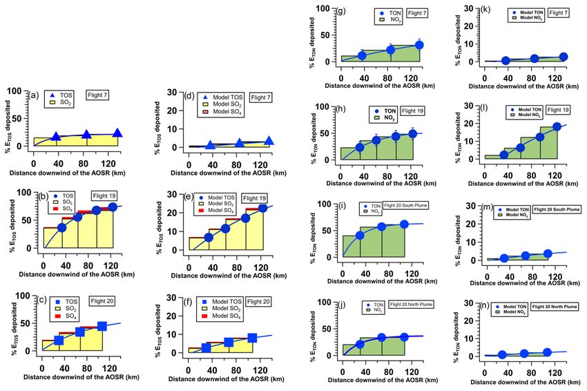
8378                                        K. Hayden et al.: Short atmospheric lifetimes of S and N due to dry deposition

for pollutants for which fast-response instruments are avail-     2016; Li et al., 2017; Liggio et al., 2019; Baray et al.,
able. However, these results are only valid for the foot-         2018). Briefly, an instrumented National Research Council
prints of the observation sites, typically hundreds of metres     of Canada Convair-580 research aircraft was flown over the
(Aubinet et al., 2012), and their extrapolation to larger re-     AOSR in Alberta, Canada, from 13 August to 7 Septem-
gions may suffer from representativeness issues. As a re-         ber 2013. The flights were designed to determine emis-
sult, atmospheric lifetimes τ with respect to dry deposi-         sions from mining activities in the AOSR, assess their atmo-
tion have not been determined through direct observations.        spheric transformation processes and gather data for satel-
On a regional scale, dry deposition fluxes are typically de-      lite and numerical model validation. Three flights were flown
rived using an inferential approach by multiplying network-       to study transformation and deposition processes by flying a
measured or model-predicted air concentrations with dry de-       Lagrangian pattern so that the same pollutant air mass was
position velocities (Vd ) (Sickles and Shadwick, 2015; Fowler     sampled at different time intervals downwind of emission
et al., 2009; Meyers et al., 1991), which are derived using       sources for a total of 4–5 h and up to 107–135 km downwind
resistance-based inferential dry deposition algorithms (Wu        of the AOSR sources. Flights 7 (F7, 19 August), 19 (F19,
et al., 2018) and compared with limited micrometeorologi-         4 September) and 20 (F20, 5 September) took place during
cal flux measurements (Wesley and Hicks, 2000; Wu et al.,         the afternoon when the boundary layer was well established.
2018; Finkelstein et al., 2000; Matsuda et al., 2006; Makar et    The flights were conducted in clear-sky conditions, so wet
al., 2018) for validation. When applied to a regional scale, an   deposition processes were insignificant. As shown in Fig. 1,
inferential-algorithm-derived Vd may have significant uncer-      the aircraft flew tracks perpendicular to the oil sands plume at
tainties (Wesley and Hicks, 2000; Aubinet et al., 2012; Wu        multiple altitudes between 150 and 1400 m a.g.l. and multi-
et al., 2018; Finkelstein et al., 2000; Matsuda et al., 2006;     ple intercepts of the same plume downwind. Vertical profiles
Makar et al., 2018; Brook et al., 1997). For example, inferred    conducted as spirals were flown at the centre of the plume
Vd for SO2 , despite being the most studied and best esti-        which provided information on the boundary layer height and
mated, may be underestimated by 35 % for forest canopies          extent of plume mixing. The flight tracks closest to the AOSR
(Finkelstein et al., 2000). Underestimated Vd for SO2 and         intercepted the main emissions from the oil sands operations;
nitrogen oxides can contribute to model overprediction of re-     there were no other anthropogenic sources as the aircraft flew
gional and global SO2 concentrations (Solomon et al., 2007;       further downwind of the AOSR.
Christian et al., 2015; Chin et al., 2000) or underprediction
of global oxidized nitrogen dry deposition fluxes (Paulot et      2.2   Aircraft measurements
al., 2018; Dentener et al., 2006).
   Here, a new approach is presented to determine τ with re-      A comprehensive suite of detailed gas- and particle-phase
spect to dry deposition and F for total oxidized sulfur (TOS,     measurements was made from the aircraft. Measurements
the sulfur mass in SO2 and particle SO4 – pSO4 ) and to-          pertaining to the analysis in this paper are discussed below.
tal reactive oxidized nitrogen (TON, the nitrogen mass in           – SO2 and NOy . Ambient air was drawn in through a
NO, NO2 , and others designated as NOz ) on a spatial scale           6.35 mm (1/4”) diameter perfluoroalkoxy (PFA) sam-
of (3 − 6) × 103 km2 , using aircraft measurements. This ap-          pling line taken from a rear-facing inlet located on
proach provides a unique methodology to determine τ and F             the roof towards the rear of the aircraft. The inlet was
over a large region. Coupled with analyses for chemical reac-         pressure-controlled to 770 mm Hg using a combination
tion rates (for TOS compounds), the average Vd for TOS and            of a MKS pressure controller and a Teflon pump. Am-
TON over the same spatial scale was also determined. The              bient air from the pressure-controlled inlet was fed to
airborne measurements were obtained during an intensive               instrumentation for measuring SO2 and NOy . The to-
campaign from August to September 2013 in the Athabasca               tal sample flow rate was measured at 4988 cm3 min−1 ,
Oil Sands Region (AOSR) (Gordon et al., 2015; Liggio et               of which SO2 and NOy were 429 and 1085 cm3 min−1 ,
al., 2016; Li et al., 2017; Baray et al., 2018; Liggio et al.,        respectively. SO2 was detected via pulsed fluores-
2019) in northern Alberta, Canada. Direct comparisons with            cence with a Thermo 43iTLE (Thermo Fisher Scien-
modelled dry deposition estimates are made to assess their            tific, Franklin, MA, USA). NOy (also denoted as TON)
uncertainties and the spatial–temporal scales of air pollutant        was measured by passing ambient air across a heated
impacts.                                                              (325 ◦ C) molybdenum converter that reduces reactive
                                                                      nitrogen oxide species to NO. NO was then detected
                                                                      through chemiluminescence with a modified Thermo
2     Methods                                                         42iTL (Thermo Fisher Scientific, Franklin, MA, USA)
                                                                      run in NOy mode. An inlet filter was used for SO2 to
2.1    Lagrangian flight design                                       exclude particles, but NOy was not filtered prior to the
                                                                      molybdenum converter. NOy includes NO, NO2 , HNO3
Details of the airborne measurement program have been                 and other oxides of nitrogen such as peroxy acetyl ni-
described elsewhere (Gordon et al., 2015; Liggio et al.,              trate and organic nitrates (Dunlea et al., 2007; Williams

Atmos. Chem. Phys., 21, 8377–8392, 2021                                             https://doi.org/10.5194/acp-21-8377-2021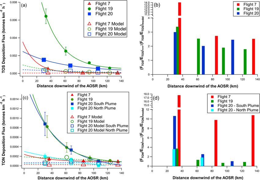
K. Hayden et al.: Short atmospheric lifetimes of S and N due to dry deposition                                                8379

Figure 1. TOS (total oxidized sulfur) and TON (total oxidized nitrogen) plumes downwind of the AOSR during three Lagrangian flights,
F7, F19 and F20. The AOSR facilities are enclosed by the yellow outline. The transfer rates T in t S or N h−1 across each screen are
shown. The grey-shaded surface areas are identified as the geographic footprint under the plumes. Data: Google Image © 2018 Image
Landsat/Copernicus.

     et al., 1998). Although there was no filter on the NOy              and HNO3 and found to be near 100 % and >90 %, re-
     inlet to exclude particles, the inlet was not designed to           spectively. Previous studies conducted by Williams et
     sample particles (i.e. rear-facing PFA tubing). As a re-            al. (1998) showed similar molybdenum converter effi-
     sult, pNO3 was not included as part of NOy (TON). The               ciencies, including that of n-propyl nitrate near 100 %.
     conversion efficiency of the heated molybdenum con-                 Interferences from alkenes or NH3 were assumed to be
     verter and inlet transmission was evaluated with NO2                negligible (Williams et al., 1998; Dunlea et al., 2007).

https://doi.org/10.5194/acp-21-8377-2021                                             Atmos. Chem. Phys., 21, 8377–8392, 2021
8380 K. Hayden et al.: Short atmospheric lifetimes of S and N due to dry deposition
Species like NO3 radical and N2 O5 are expected to be the AMS measures only particle massK. Hayden et al.: Short atmospheric lifetimes of S and N due to dry deposition 8381
quently sent to an analytical laboratory for GC-FID/MS were also extrapolated linearly to background values from
analyses for a suite of 150 hydrocarbon compounds. the highest-altitude flight tracks upwards to the mixed-layer
height, which was determined from vertical profiles of pollu-
– Meteorology and aircraft state parameters. Meteorolog-
tant mixing ratios, temperature and dew point (Table 1).
ical measurements have been described elsewhere (Gor-
Changes in the mass transfer rate T (denoted 1T ) in units
don et al., 2015). In brief, 3-D wind speed and tempera-
of t h−1 were then calculated as the differences in T between
ture were measured with a Rosemount 858 probe. Dew
pairs of virtual screens. The uncertainty in 1T was estimated
point was measured with an Edgetech hygrometer and
as 8 % for TOS and 26 % for TON, as supported by emission
pressure was measured with a DigiQuartz sensor. Air-
rate uncertainties determined for box flights (Gordon et al.,
craft state parameters including positions and altitudes
2015). The uncertainty analysis for box flights is applicable
were measured with GPS and a Honeywell HG1700
to 1T here, as both account for uncertainties with an upwind
unit. All meteorological measurements and aircraft state
and a downwind screen. The 1T uncertainties were propa-
parameters were measured at a 1 s time resolution.
gated through subsequent calculations.
2.3 Mass transfer rates in the atmosphere Knowing the change in mass transfer rate 1T and ac-
counting for the net rates of chemical loss and formation
Mass transfer rates (T ) across flight screens (Fig. 1) were between screens for SO2 and pSO4 , the deposition rates
determined using an extension of the Top-down Emission (and subsequently the deposition flux in tonnes S (or N)
Rate Retrieval Algorithm (TERRA) developed for emission km−2 h−1 , Sect. 2.4) were determined for the sulfur com-
rate determination using aircraft measurements (Gordon et pounds as follows:
al., 2015). Briefly, at each plume interception location, the
level flight tracks were stacked to create a virtual screen. 1TSO2 = TSO2 (t2 ) − TSO2 (t1 ) = XSO2 − DSO2 , (2)
Background subtracted pollutant concentrations and hori- 1TpSO4 = TpSO4 (t2 ) − TpSO4 (t1 ) = XpSO4 − DpSO4 , (3)
zontal wind speeds normal to the screen were interpolated 1TTOS = TTOS (t2 ) − TTOS (t1 ) = −DTOS , (4)
using kriging. The background for SO2 was ∼ 0 ppb, and
pSO4 was 0.2–0.3 µg m−3 , which was subtracted from the where XSO2 is the rate of chemical reaction loss of sulfur
pSO4 measurements before mass transfer rates were calcu- mass in SO2 , XpSO4 is the rate of chemical formation of sul-
lated (Liggio et al., 2016). Integration of the horizontal fluxes fur mass as pSO4 , DSO2 and DpSO4 are deposition rates of
across the plume extent on the screen yields the transfer rate sulfur mass in SO2 and pSO4 , respectively, and t1 and t2 are
T in units of t h−1 . Using SO2 as an example, plume interception times at Screen 1 and Screen 2, respec-
Z s2 Z z2 tively. Note that the chemical loss rate of SO2 is set to be
TSO2 = C (s, z) un (s, z) dsdz, (1) equivalent to the formation rate of pSO4 , i.e. XSO2 = XpSO4 .
s1 z1 Equation (4) for TOS can also similarly be written as shown
where C (s, z) is the background subtracted concentration at in Eq. (5).
screen coordinates s and z, which represent the horizontal
and vertical axes of the screen. The un (s, z) is the horizontal 1TTOS = 1TSO2 + 1TpSO4 = −DSO2 − DpSO4 (5)
wind speed normal to the screen at the same coordinates. Units in Eqs. (2) to (5) are all in t h−1 . Reaction with the OH
Since the lowest flight altitude was 150 m a.g.l., it was nec- radical was considered to be the most significant chemical
essary to extrapolate the data to the surface as per the proce- loss of SO2 and the most significant path for the formation
dures described previously (Gordon et al., 2015). Extrapo- of pSO4 . XSO2 and XpSO4 were determined using estimated
lation to the surface methods was compared and differences OH radical concentrations, which were estimated using the
were included in the uncertainty estimates. The main sources methodology described in Supplement Sect. S4. Although
of SO2 were from elevated facility stacks associated with the TON encompasses a range of different N species with ex-
desulfurization of the raw bitumen (Zhang et al., 2018). The pected differences in their deposition rates, it was not possi-
stacks with the biggest SO2 emissions range in height from ble to quantitatively separate their chemical formation/losses
76.2 to 183.0 m. Since the main source of SO2 is from the from their deposition rates with this method. For total oxi-
elevated facility stacks, the uncertainty for a single screen dized sulfur TOS (i.e. sulfur in SO2 + pSO4 ) and total ox-
is estimated at 4 % (Gordon et al., 2015). NOy was also idized nitrogen TON (i.e. nitrogen in NOy ), the chemistry
extrapolated linearly to the surface, and the mass transfer term is not relevant, and thus the dry deposition rate DTOS
rates were similarly compared to other extrapolation meth- was directly determined from 1TTOS using Eq. (4) and, re-
ods. NOy sources include the elevated facility stacks and sur- spectively, for TON.
face sources such as the heavy hauler trucks operating in the
surface mines. The uncertainty in the resulting transfer rate T 2.4 Dry deposition fluxes and dry deposition velocities
for a single screen is estimated to be larger at 8 %, as a larger
fraction of the NOy mass may be below the lowest measure- Average dry deposition fluxes (F ) for TOS and TON were
ment altitude (Gordon et al., 2015). Sulfur and nitrogen data obtained by dividing the deposition rates D in t h−1 by the
https://doi.org/10.5194/acp-21-8377-2021 Atmos. Chem. Phys., 21, 8377–8392, 20218382 K. Hayden et al.: Short atmospheric lifetimes of S and N due to dry deposition
Table 1. Average observed meteorological conditions and facility emission rates of TOS (ETOS ) and TON (ETON ) (determined from ex-
trapolated (to distance = 0) transfer rates; Fig. 1) for TOS and TON during the F7, F19 and F20 flights. SP: southern plume; NP: northern
plume.
Flight Date Time Mean wind Mean wind Mixed-layer ETOS ETON
(UTC) speed (m s−1 ) direction (◦ ) height (m a.g.l.) (t h−1 ) (t h−1 )
7 19 Aug 2013 20:07–01:08 13.0 ± 1.0 256 ± 11.7 2500 ± 100 3.4 1.2
19 4 Sep 2013 18:54–23:53 9.5 ± 1.9 218 ± 16 1200 ± 100 18.5 3.9
20 5 Sep 2013 19:33–24:36 8.9± 1.2 281± 11 2100± 100 5.8 2.2 (SP)
1.2 (NP)
footprint surface area of the plume between two adjacent is used in the calculation of Vd since the deposition behaviour
screens (Fig. 1 grey-shaded regions), as shown in Eq. (6) for of gases and particles differs substantially, and particles ad-
the dry deposition flux FTOS of TOS (in t S km−2 h−1 ): ditionally have size-dependent deposition rates (Emerson et
DTOS al., 2020). As the dominant form of TOS is SO2 (>92 %), the
FTOS = , (6) deposition behaviour of TOS is expected to be largely driven
Area
by that of SO2 . The measured TON does not include pNO3 .
where the surface area, Area, was identified as the geographic
area under the plume extending to the edges of the plume FSO2
Vd = (7)
where concentrations fell to background levels (i.e. SO2 to [SO2 ]
∼ 0 ppb; SO4 ∼ 0.2 µg m−3 ). This approach was similarly The largest source of uncertainty in Vd calculated this way
used to derive deposition fluxes from an air quality model, was the determination of concentration at 40 m above the sur-
Global Environmental Multiscale – Modelling Air-quality face as the measurements were extrapolated from the lowest
and Chemistry (GEM-MaCH) (Moran et al., 2014; also see aircraft altitude to the surface and interpolated concentrations
Supplement Sect. S5 for details). The geographic surface were used. The measurement-derived Vd are compared with
area uncertainty is estimated at 5 %. Dry deposition fluxes those from the air quality model GEM-MACH, which uses
between the sources and the first screen were also estimated inferential methods.
using change in mass transfer rate 1T based on the extrap-
olated transfer rates back to the source region (“extended” 2.5 Monte Carlo simulations of dry deposition
region). The surface area boundaries for these “extended” re- velocities using multiple resistance-based
gions were determined using latitude and longitude coordi- parameterizations
nates that were weighted by emissions. This was done by first
using the average wind direction from Screen 1 and creating Parameterization of dry deposition in inferential algorithms
a set of parallel back trajectories (∼ 20) starting at different is commonly based on a resistance approach with dry depo-
parts of Screen 1 back across the source region. For TON, sition velocity depending on three main resistance terms as
the NOx emission sources along each back trajectory were below:
weighted by their NOx emissions to obtain an emissions- 1
weighted centre location with latitude and longitude coor- Vd = , (8)
Ra + Rb + Rc
dinates for each back trajectory. The line connecting these
emissions-weighted centre locations formed the boundary of where Ra , Rb and Rc represent the aerodynamic, quasi-
the extended surface area. The extended surface area was laminar sublayer and bulk surface resistances, respectively.
similarly determined for TOS based upon the known loca- Although these resistance terms are common among many
tions of the major SO2 point sources. The uncertainty of the regional air quality models (Wu et al., 2018), the formulae
“extended” regions is estimated at 10 % based on repeated used (and inputs into these formulae) to calculate the in-
optimizations of the geographical area. Surface areas are vi- dividual resistance terms differ significantly among the in-
sualized as grey-shaded regions between screens in Fig. 1 ferential deposition algorithms. To assess the potential for a
and tabulated in Supplement Table S1. general underestimation of Vd across different inferential de-
Spatially averaged dry deposition velocities, Vd , based on position algorithms and to compare with the aircraft-derived
the aircraft measurements were determined over the surface Vd , five different inferential deposition algorithms, including
area between screens using average plume concentrations that used in the GEM-MACH model for calculating Vd (Wu
across pairs of screens at about 40 m above the ground for et al., 2018), were incorporated into a Monte Carlo simula-
SO2 and TON (e.g. Eq. 7 for SO2 in units of cm s−1 ). Al- tion for Vd for SO2 . NOy was not considered here, as its mea-
though TOS includes the S in both SO2 and pSO4 , only SO2 surement includes multiple reactive nitrogen oxide species
Atmos. Chem. Phys., 21, 8377–8392, 2021 https://doi.org/10.5194/acp-21-8377-2021K. Hayden et al.: Short atmospheric lifetimes of S and N due to dry deposition 8383
with different individual deposition velocities. We note that downwind. The main sources of nitrogen oxides were from
many of the inferential algorithms are based on observations exhaust emissions from off-road vehicles used in open pit
of SO2 and O3 deposition made at single sites, and the extent mining activities and sulfur and nitrogen oxides from the el-
to which a chemical is similar to SO2 or O3 features in its Vd evated facility stack emissions associated with the desulfur-
calculation – the comparison thus has relevance for species ization of raw bitumen (Zhang et al., 2018). As depicted in
aside from SO2 . The five deposition algorithms considered Fig. 1, F7 and F19 captured a plume that contained both sul-
are denoted ZHANG, NOAH-GEM, C5DRY, WESLEY and fur and nitrogen oxides. The westerly wind direction and ori-
GEM-MACH and are compared in Wu et al. (2018) (except entation of the aircraft tracks on F20 resulted in the measure-
the algorithm in GEM-MACH). The five algorithms all use a ment of two distinct plumes: one plume exhibited increased
big-leaf approach for calculating Vd ; i.e. Vd is based on the levels of sulfur and nitrogen oxides mainly from the facility
resistance-analogy approach for calculating dry deposition stacks and the other plume contained elevated levels of nitro-
velocity, where Vd is the reciprocal sum of three resistance gen oxides, mainly from the open pit mining activities, and
terms Ra , Rb and Rc . Although the approach is similar, the no SO2 .
formulations of Ra , Rb and Rc between the algorithms are During the experiments, the dry deposition rates (D)
substantially different (Table 1 in Wu et al., 2018). Results (t h−1 ) were quantified under different meteorological con-
from Wu et al. (2018) suggest that the differences in Ra + Rb ditions and emissions levels of TOS and TON (ETOS and
between different models would cause a difference in their Vd ETON ) for the three flights (see Table 1). These differences
values of the order of 10 %–30 % for most chemical species played important roles in the observed pollutant concentra-
(including SO2 and NO2 ), although the differences can be tions and resulting dry deposition fluxes for F7, F19 and F20.
much larger for species with near-zero Rc such as HNO3 . Mixed-layer heights (MLHs) were derived from aircraft ver-
To perform the simulations, formulae for the first four al- tical profiles that were conducted in the centre of the plume at
gorithms were taken from Wu et al. (2018) and for GEM- each downwind set of transects. The profiles of temperature,
MACH taken from Makar et al. (2018). The stomatal resis- dew point temperature, relative humidity and pollutant mix-
tance in the ZHANG algorithm was from Zhang et al. (2002). ing ratios were inspected for vertical gradients, indicating a
The GEM-MACH formula (Eq. 8.7 in the Supplement of contiguous layer connected to the surface. The highest MLH
Makar et al., 2018) for mesophyll resistance Rmx contained a was determined for F7 at 2500 m a.g.l., whereas F19 had the
typo (missing the Leaf Area Index – LAI) and was corrected lowest MLH at 1200 m a.g.l. (Table 1). In F20, the MLH was
for as follows. 2100 m a.g.l. The combination of a high MLH in F7 with the
−1 highest wind speeds resulted in the lowest pollutant concen-
Rmx = LAI H ∗ /3000 + 100f0
(9) trations of the three flights. In F19, lower wind speeds and the
lowest mixed-layer heights led to the highest pollutant levels.
Prescribed input values were constrained by the range of pos- F20 had emissions and meteorological conditions that were
sible values consistent with the conditions during the aircraft in between F7 and F19, resulting in pollutant concentrations
flights and are shown in Supplement Table S3 with associ- between those of F7 and F19.
ated references. Calculations for the Ra term were based on Emission rates of SO2 and NOx (designated as ETOS and
unstable and dry conditions as observed during the aircraft ETON ) from the main sources in the AOSR were estimated
flights. The Monte Carlo simulation generated a distribution from the aircraft measurements and varied significantly be-
of possible Vd values, based on randomly generated values of tween the 3 flight days. The measurement-based emission
the input variables to each algorithm and selected from Gaus- rates of ETOS and ETON were taken from the mass transfer
sian distributions with a range of 3σ for all input parameters. rates of TSO2 and TNOy (described in Methods) by extrapo-
All simulations were performed with the same input values lating backwards to the source locations in the AOSR using
that were common between the algorithms. exponential functions (Fig. 2, Sect. 3.2). For TOS, the source
location was set at 57.017◦ N, −111.466◦ W, where the main
3 Results and discussion stacks for SO2 emissions are located. For TON, the source
locations were determined from geographically weighted lo-
3.1 Meteorological and emissions conditions during the cations. Emission rates ETOS and ETON for each flight are
transformation flights shown in Table 1.
Model-based ETOS and ETON were also obtained from the
Three aircraft flights, Flights 7 (F7), 19 (F19) and 20 (F20), 2.5 km × 2.5 km gridded emissions fields that were specifi-
were conducted in Lagrangian patterns where the same cally developed for model simulations of the large AOSR sur-
plume emitted from oil sands activities was repeatedly sam- face mining facilities (Zhang et al., 2018), i.e. Suncor Millen-
pled for a 4–5 h period and up to 107–135 km downwind nium, Syncrude Mildred Lake, Syncrude Aurora North, Shell
of the AOSR. The first screen of each flight captured the Canada Muskeg River Mine & Muskeg River Mine Expan-
main emissions from the oil sands operations with no ad- sion, CNRL Horizon Project and Imperial Kearl Mine. The
ditional anthropogenic sources between subsequent screens emissions fields have been used in GEM-MACH (described
https://doi.org/10.5194/acp-21-8377-2021 Atmos. Chem. Phys., 21, 8377–8392, 20218384 K. Hayden et al.: Short atmospheric lifetimes of S and N due to dry deposition
to 107–135 km downwind of the sources. Curves were fit-
ted to the TOS and TON dry deposition cumulative percent-
ages from which d1/e and τ were determined (Supplement
Table S1). The transport e-folding distance (d1/e ) was deter-
mined where 63.2 % of ETOS (or ETON ) was dry deposited,
Pd1/e
i.e. d=0 D(d) = 0.368ETOS . The atmospheric lifetimes (τ )
were derived as τ = d1/e /u, where u was the average wind
speed across the distance d1/e . These estimates were com-
pared with predictions from the regional air quality model
GEM-MACH (Makar et al., 2018; Moran et al., 2014; Sup-
plement Sect. S5) using facility emission rates (Table 2). For
TOS during F19 (Fig. 3b, e), the observed cumulative depo-
sition at the maximum distance accounted for 74 ± 5 % vs.
the modelled 21 % of ETOS . The measurements indicate that
the cumulative deposition of TOS was due mostly to SO2
dry deposition, where SO2 was ∼ 100 % of TOS closest to
the oil sands sources, decreasing to 94 % farthest downwind.
Although the modelled cumulative deposition of TOS was
significantly lower than the observations, the fractional de-
position of SO2 was similar, decreasing from ∼ 100 % to
95 % of TOS. Fitting a curve to D and interpolating the cu-
mulative deposition fraction to the 63.2 % ETOS loss leads
to a d1/e of 71 ± 1 km vs. 500 km for the model predic-
tion. Under the prevailing wind conditions, the observed dis-
tance indicates a τ for TOS of approximately 2.2 h, whereas
the model prediction indicated 16 h. Large observation-based
values and model prediction differences in lifetime were also
Figure 2. TERRA-derived transfer rates of (a) TOS and (b) TON evident for the other flights (Supplement Table S1). Clearly,
for F7, F19 and F20. The vertical bars indicate the propagated un- the model predictions significantly underestimated deposi-
certainties. The model emission rates ETOS and ETON are shown tion and vastly overestimated d1/e and τ . The observation-
by the open symbols. based values for τ are also lower than average lifetimes of
1–2 d for SO2 and 2–9 d for pSO4 derived from global mod-
els (Chin et al., 2000; Benkovitz et al., 2004; Berglen et al.,
in Supplement Sect. S5) to carry out a number of model sim- 2004), which include the effects of wet deposition and chem-
ulations (Zhang et al., 2018; Makar et al., 2018), including ical conversion for SO2 , thus making their implicit residence
for the present study. In this work, emissions were summed times with respect to dry deposition even longer.
from various sources, including off-road, point (continuous For TON in F19 (Fig. 3h, l), the observed cumulative
emissions monitoring – CEMS), and point (non-CEMS), for deposition accounted for 49 ± 11 % of ETON at the maxi-
the surface mines to obtain total AOSR hourly emission rates mum flight distance vs. 19 % predicted by the model. Sim-
for the flight time periods of interest (Table 2). The standard ilar model underestimates for cumulative deposition frac-
deviations reflect the emissions variations during the simu- tions were found for F7 and F20. Extrapolating to the 63.2 %
lated flight. cumulative deposition fraction, d1/e was estimated to be
190 ± 7 km for F19 vs. a predicted 650 km from the model,
3.2 Mass transfer rates implying a τ of approximately 5.6 h for the measurement-
based results and 23 h for the model prediction. Again, anal-
The mass transfer rates T (in t h−1 ) across the virtual flight ogous differences for F7 and F20 were found (Supplement
screens for all three flights are shown for TOS and TON in Table S1). Similar to TOS, the measurement-based d1/e and
Fig. 1 and plotted in Fig. 2. In F20, two distinct TON plumes τ values for TON were significantly smaller than commonly
were observed, allowing separate T calculations for TON. accepted lifetimes of a few days for nitrogen oxides in the
Monotonic decreases in T were observed for both TOS and boundary layer (Munger et al., 1998).
TON during transport downwind in all flights, clearly show-
ing dry depositional losses. The deposition rate D (Methods, 3.3 Dry deposition fluxes F
Sect. 2.3) was used to estimate the cumulative deposition of
TOS and TON as a fraction of ETOS or ETON and is shown Using the deposition rate D (in tonnes S or N h−1 ), the av-
in Fig. 3 for F7, F19 and F20 for transport distances of up erage dry deposition fluxes, F (in tonnes S or N km−2 h−1 ),
Atmos. Chem. Phys., 21, 8377–8392, 2021 https://doi.org/10.5194/acp-21-8377-2021K. Hayden et al.: Short atmospheric lifetimes of S and N due to dry deposition 8385
Table 2. Model average meteorological conditions and facility emission rates of TOS (ETOS ) and TON (ETON ) during the F7, F19 and F20
flights as described above. SP: southern plume; NP: northern plume.
Flight Date Time Mean wind Mean wind Mixed-layer ETOS ETON
(UTC) speed (m s−1 ) direction (◦ ) height (m a.g.l.) (t h−1 ) (t h−1 )
7 19 Aug 2013 20:07–01:08 12.6 ± 0.3 253 ± 5.0 1670 ± 80 3.8 2.9
19 4 Sep 2013 18:54–23:53 8.1 ± 1.0 225 ± 4.6 1450 ± 43 4.3 2.4
20 5 Sep 2013 19:33–24:36 9.1 ± 0.7 275 ± 1.6 1590 ± 42 3.7 1.5 (SP)
0.9 (NP)
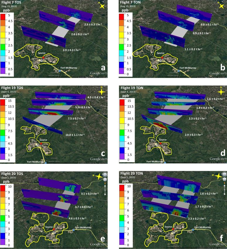
Figure 3. Cumulative dry deposition as a percentage of emissions ETOS (a to f) or ETON (g to n) for F7, F19 and F20 measurements with
corresponding GEM-MACH model predictions. The bars show the dry deposition due to SO2 and pSO4 . The curves were fitted to the TOS
and TON dry deposition percentages from which d1/e and τ were determined.
were calculated by dividing D by the plume footprint surface distances for FTOS of 18, 27, and 55 km for F7, F19, and
areas estimated by extending to the plume edges where the F20, respectively. More than 90 % of the decreases in FTOS
concentrations fell to background levels (Methods, Sect. 2.4). were accounted for by FSO2 . Similarly, FTON decreased ex-
These footprints are shown as the grey-shaded geographic ar- ponentially with increasing transport distances in all flights
eas in Fig. 1, totalling 3500, 5700, and 4200 km2 for the F7, (Fig. 4c), exhibiting e-folding distances of 18 and 33 km for
F19, and F20 plumes, respectively; see Supplement Table S1 F7 and F19 and 55 and 189 km for the southern and north-
for TON plume areas). Figure 4a shows FTOS values for all ern TON plumes during F20, respectively. These e-folding
three flights, exhibiting exponential decreases with increas- distances were similar to those for FTOS , indicating similar
ing distance away from the sources and showing e-folding rates of decreases in FTON with transport distances.
https://doi.org/10.5194/acp-21-8377-2021 Atmos. Chem. Phys., 21, 8377–8392, 20218386 K. Hayden et al.: Short atmospheric lifetimes of S and N due to dry deposition Figure 4. Dry deposition fluxes FTOS and FTON (in t km−2 h−1 ) determined from measurements (solid symbols) and GEM-MACH model predictions (open symbols). (a) FTOS , (b) ratios of measurement-to-model normalized emissions FTOS /ETOS , (c) FTON , and (d) ratios of measurement-to-model normalized emissions FTON /ETON . The potential for other processes to contribute to the de- flux (= FTOS /ETOS and FTON /ETON ) was calculated for rived TOS and TON fluxes were considered, including losses both measurement and model (Supplement Fig. S2). Fig- from the boundary layer to the free troposphere and re- ure 4b shows the ratios of measurement-to-model normalized emission of TOS or TON species from the surface back emissions for TOS. The model emission-normalized fluxes to the gas phase. Two different approaches, a finite-jump FTOS /ETOS were lower than the measurement-based values model and a gradient flux approach (Stull, 1988; Degrazia by factors of 2.5–14, 1.8–3.4, and 2.0–3.0 for F7, F19, and et al., 2015), were used to estimate the potential upward F20, respectively, decreasing with increased transport dis- loss across the interface between the boundary layer and the tances. However, they coalesce to a factor of 2 at the furthest free troposphere for sulfur and nitrogen. In both approaches, distances sampled by the aircraft, indicating that the model the upward S flux was a minor loss at 10×) (Fig. 4d). and measurement FTOS could be explained by differences in actual vs. model emissions, ETOS (Tables 1 vs. 2). To remove the influence of emissions, an emission-normalized Atmos. Chem. Phys., 21, 8377–8392, 2021 https://doi.org/10.5194/acp-21-8377-2021
K. Hayden et al.: Short atmospheric lifetimes of S and N due to dry deposition                                            8387

3.4   Dry deposition velocities Vd                               ods Sect. 2.5. Results for the Vd simulation algorithms are
                                                                 shown in Fig. 5a. Histograms for all five algorithms have
The shorter d1/e and τ and larger deposition fluxes F near       peak Vd values at ∼ 1 cm s−1 or lower. Probability distri-
the sources determined from the aircraft measurements com-       butions for the individual resistance terms Ra , Rb , and Rc
pared to predictions by the GEM-MACH model indicate that         showed that the dominant resistance driving Vd was the Rc
the model dry deposition velocities Vd were underestimated.      term (Supplement Fig. S3). Also shown in Fig. 5a are the
Gas-phase Vd in the model is predicted with a standard infer-    measurement-derived Vd for Flights 7, 19 and 20 and that
ential “resistance” algorithm (Wesley, 1989; Jarvis, 1976),      from the Oski-ôtin ground site. The observed Vd values are
with resistance to deposition calculated for multiple parame-    larger than the Vd values for most of the simulations, with the
ters, including aerodynamic, quasi-laminar sublayer and bulk     exception of Flight 7, where the Zhang et al. (2002), NOAH-
surface resistances (Baldocchi et al., 1987). To demonstrate     GEM (Wu et al., 2018) and C5DRY (Wu et al., 2018) al-
the model underestimation in Vd , comparisons between the        gorithms’ distributions agree with the observations. All al-
measurement-based and model Vd were made where an eval-          gorithms are biased low relative to the observations for the
uation of Vd for TOS and TON was possible. All FSO2 were         remaining flights and the Oski-ôtin ground site. It is noted
converted into Vd−SO2 by dividing FSO2 by interpolated SO2       that the ground-site observations that were derived using a
concentrations at 40 m above ground, averaging 1.2 ± 0.5,        standard flux tower methodology (Supplement Sect. S3) at
2.4 ± 0.4, and 3.4 ± 0.6 cm s−1 for F7, F19, and F20, respec-    a single site appeared to be higher than all other Vd ; nev-
tively, across the plume footprints (Methods Sect. 2.4 and       ertheless, these observations are closer to the aircraft values
Supplement Table S2). The corresponding model Vd−SO2 de-         than the algorithm estimates. These results indicate that an
rived in the same way as the observations was 0.72, 0.63,        underestimation of Vd relative to both aircraft and ground-
and 0.58 cm s−1 , 1.7–5.4 times lower than observations (Sup-    based measurements in the AOSR is not unique to the GEM-
plement Sect. S5; Supplement Table S2). Interestingly, the       MACH model or its dry deposition algorithm; similar results
median Vd for SO2 of 4.1 cm s−1 determined using eddy co-        would occur with the other algorithms included in the Monte
variance/vertical gradient measurements from a tower in the      Carlo simulations, all of which are used within other regional
AOSR is higher than the mass-balanced method, showing            models.
an even larger discrepancy compared to the model (Supple-           To investigate the possible reasons behind the low model
ment Sect. S3; Fig. S5). Similarly, derived Vd−TON averaged      Vd relative to the observations, a series of sensitivity tests
2.8 ± 0.8, 1.6 ± 0.5, 4.7 ± 1.4, and 2.2 ± 0.7 cm s−1 for the    using SO2 were conducted. Differences in model Vd have
F7, F19, and F20 southern plumes and F20 northern plume,         been shown to be mainly due to differences in the calcu-
respectively (Supplement Table S2), 1.2–5.2 times higher         lated Rc (Wu et al., 2018), and sensitivity tests here indi-
than the corresponding modelled Vd−TON of 1.4, 1.3, 0.92,        cated that Rc is particularly sensitive to the cuticular resis-
and 0.90 cm s−1 .                                                tance Rcut . Hence, factors causing Rcut to change can have
   Using the observations, it was not possible to derive in-     significant impact on model Vd . In some of the algorithms,
dividual TON deposition rates separate from their chemi-         Rcut and other resistance terms are dependent on the effec-
cal formation/losses. In previous modelling work, Makar et       tive Henry’s law constant KH ∗ for SO2 . The Monte Carlo
al. (2018) use the GEM-MACH model and describe the rela-         simulations for Fig. 5 assumed a surface pH = 6.68 resulting
tive contributions of different TOS and TON species towards      in a KH ∗ of 1 × 10⁵ for SO2 . Additional Monte Carlo sim-
total S and N deposition in the AOSR. TON was dominated          ulations were performed for the GEM-MACH dry deposi-
by dry NO2 (g) dry deposition fluxes close to the sources        tion algorithm by adjusting KH ∗ assuming different pH with
(>70 % of total N close to the sources), and dry HNO3 (g)        small variations from a pH = 6.68 significantly changing Rc ,
dry deposition increases with increasing distance from the       Rcut , and Vd (Supplement Fig. S4). In Fig. 5b – red dashed
sources (remaining
8388 K. Hayden et al.: Short atmospheric lifetimes of S and N due to dry deposition
net flux of all processes including the effects of deposition
and any potential re-emissions of TOS and TON compounds
should this process occur. As the results show a net down-
ward flux (i.e. net deposition), if any re-emission was occur-
ring, it would be smaller than the deposition fluxes observed
here, which are themselves higher than shown by currently
available deposition algorithms. This implies that the deposi-
tion part of the flux must be even larger than the net observed
flux, and the measured net fluxes presented here should then
be considered minimum values. The current deposition al-
gorithms do not include bidirectional fluxes for inorganics,
and adjustments related to pH in some situations may not be
sufficient to parameterize deposition fluxes. A bidirectional
approach may be needed that would include not only [H+ ],
but also surface heterogeneous reactions, to determine near-
surface equilibrium concentrations of co-depositing gases
such as ammonia and nitric acid.
It is clear that from the Monte Carlo simulations for
SO2 Vd comparisons, inferential dry deposition algorithms
as used in regional and global chemical transport models
need to be further validated and improved, especially over
large geographic regions. Here, the role of pH was identi-
fied for improvement in some algorithms along with possible
improvement in aerodynamic and quasi-laminar sublayer re-
sistance parameters. Yet for other algorithms and for TON
compounds, the model low biases in Vd remain to be investi-
gated.
The underestimates suggest that the applications of these
Figure 5. (a) Distributions of Vd for SO2 from Monte Carlo simu- algorithms in regional or global models may significantly un-
lations using five different deposition parameterizations (Wu et al., derestimate predictions of TOS dry depositional loss from
2018; Makar et al., 2018) and (b) Monte Carlo simulations for the the atmosphere. Underestimates in Vd are the result of a com-
GEM-MACH algorithm using a pH = 8 and using a pH = 8 plus re- bination of uncertainties in the parameterizations of each al-
placing the GEM-MACH algorithm Ra and Rb formulae with that gorithm. In the case of the algorithm used in GEM-MACH,
from Zhang et al. (2002) and NOAH-GEM (Wu et al., 2018), re- by adjusting the assumed surface pH from 6.68 to 8 (jus-
spectively. Aircraft-derived Vd for F7, F19 and F20 as well as the tifiable given the considerable dust emissions in the re-
median value for the Oski-ôtin ground site (Supplement Fig. S5) are gion: Zhang et al., 2018), the model Vd moved closer to
shown in both (a) and (b) for comparison.
the aircraft-derived values (Fig. 5b), reducing the model–
observation gap by approximately two-thirds. In addition,
substituting the aerodynamic resistance and quasi-laminar
current deposition velocity algorithms. By using the Zhang sublayer resistance parameterizations in the GEM-MACH al-
et al. (2002) Ra and the NOAH-GEM (Wu et al., 2018) Rb gorithm with that from Zhang et al. (2002) and NOAH-GEM
parameterizations in the GEM-MACH algorithm, a further (Wu et al., 2018), respectively, resulted in a further increase
shift of the GEM-MACH Vd distribution to larger values was in the model Vd distribution that encompasses most of the
found, with the range encompassing most of the observations observations (Fig. 5b). Clearly, different algorithms respond
(Fig. 5b, pink dashed line). Using the Zhang and NOAH- differently to changes in the parameterizations, and valida-
GEM parameterizations, rather than the GEM-MACH pa- tion and adjustment to each algorithm need measurement-
rameterization, would decrease the Ra and Rb for the mo- based results over large regions such as derived here.
mentum, heat and moisture fluxes as well but still remain
within the range of what is expected based on published pa-
rameterizations (Wu et al., 2018, and references therein). 4 Conclusions
The potential for re-emission of TOS and TON species
was also considered. Fulgham et al. (2020) report that the The atmospheric transport distances and lifetimes d1/e and τ
bidirectional fluxes of volatile organic acids are driven by determined from the aircraft measurements are substantially
an equilibrium partitioning between surface wetness and the shorter than the GEM-MACH model predictions, and the dry
atmosphere. The observations presented here represent the deposition fluxes F and velocities and Vd near sources are
Atmos. Chem. Phys., 21, 8377–8392, 2021 https://doi.org/10.5194/acp-21-8377-2021K. Hayden et al.: Short atmospheric lifetimes of S and N due to dry deposition 8389
larger compared to the predictions by GEM-MACH and five environment-climate-change/services/oil-sands-monitoring/
inferential dry deposition velocity algorithms, respectively. monitoring-air-quality-alberta-oil-sands.html (Government of
There are important implications for these measurement– Canada, 2019).
model discrepancies. Such discrepancies indicate that re-
gional or global chemical transport models using these algo-
rithms are biased low for local deposition and high for long- Supplement. The supplement related to this article is available on-
range transport and deposition, and TOS and TON losses line at: https://doi.org/10.5194/acp-21-8377-2021-supplement.
from the atmosphere are significantly underpredicted, result-
ing in overestimated lifetimes. While the measurements took
Author contributions. KH, SML, JL, SGM, RM, RMS, JO’B and
place over a relatively short time period, these results indicate
MW all contributed to the collection of aircraft observations in the
that TOS and TON may be removed from the atmosphere at field. KH, RM and JO’B made the SO2 , NOy and pSO4 measure-
about twice the rate as predicted by current atmospheric de- ments and carried out subsequent QA/QC of data. RM analysed can-
position algorithms. This, in turn, implies a potentially sig- ister VOCs and provided OH concentration estimates. RMS made
nificant impact on deposition over longer timescales (poten- and provided the ground-site deposition velocity measurements.
tially weeks to months) and relevance towards cumulative AD contributed to the development of TERRA. JL wrote the Monte
environmental exposure metrics such as critical loads and Carlo code. PM and AA ran the model and provided model analy-
their exceedance. A faster near-source deposition velocity for ses. JZ provided emissions data. LZ and RMS provided deposition
emitted reactive gases may imply less S and N mass being algorithm parameters. KH and SML wrote the paper input from all
available for long-range transport, reducing concentrations the co-authors.
and deposition further downwind. The near-source higher de-
position velocity thus has the important implication of a re-
duction in more distant and longer timescale deposition for Competing interests. The authors declare that they have no conflict
of interest.
locations further from the sources. Moreover, emissions as-
sessed through network measurements or budget analysis of
atmospheric TOS and TON (Sickles and Shadwick, 2015;
Acknowledgements. The authors thank the National Research
Paulot et al., 2018; Berglen et al., 2004) may be underesti-
Council of Canada flight crew of the Convair-580, the Air Quality
mated due to lower Vd used in these estimates and may re- Research Division technical support staff, Julie Narayan for in-field
quire reassessment of the effectiveness of control policies. data management support, and Stewart Cober for the management
Shorter τ for TOS and TON reduces their atmospheric spa- of the study.
tial scale and intensity of smog episodes, potentially reducing
human exposures (Moran et al., 2014). Importantly, shorter τ
for TOS and TON reduces their contribution to atmospheric Financial support. The project was funded by the Air Quality pro-
aerosols; consequently, the negative direct and indirect ra- gram of Environment and Climate Change Canada and the Oil
diative forcing from these sulfur and nitrogen aerosols is re- Sands Monitoring (OSM) program. It is independent of any posi-
duced, reducing their cooling effects on climate (Solomon et tion of the OSM program.
al., 2007). These impacts suggest that more measurements
to determine τ and F for these pollutants across large geo-
graphic scales and different surface types are necessary for Review statement. This paper was edited by Barbara Ervens and
better quantifying their climate and environmental impacts reviewed by two anonymous referees.
in support of policy. While in the past such determination
was difficult and/or impossible, the present study provides a
viable methodology to achieve such a goal.
References
Code availability. All the computer code associated with the Aubinet, M., Vesala, T., and Papale, D. (Eds.): Eddy Covari-
TERRA algorithm, including for the kriging of pollutant data, ance, Springer Atmospheric Sciences, Springer, Dordrecht, The
a demonstration dataset and associated documentation are freely Netherlands, 2012.
available upon request. The authors request that future publications Baldocchi, D. D., Vogel, C. A., and Hall, B.: A canopy stomatal
which make use of the TERRA algorithm cite this paper, Gordon et resistance model for gaseous deposition to vegetated surfaces,
al. (2015), Liggio et al. (2016), or Li et al. (2017) as appropriate. Atmos. Environ., 21, 91–101, https://doi.org/10.1016/0004-
6981(87)90274-5, 1987.
Baray, S., Darlington, A., Gordon, M., Hayden, K. L., Leithead,
Data availability. All data used in this publication are freely A., Li, S.-M., Liu, P. S. K., Mittermeier, R. L., Moussa, S. G.,
available on the Canada-Alberta Oil Sands Environmental O’Brien, J., Staebler, R., Wolde, M., Worthy, D., and McLaren,
Monitoring Information Portal: https://www.canada.ca/en/ R.: Quantification of methane sources in the Athabasca Oil
Sands Region of Alberta by aircraft mass balance, Atmos.
https://doi.org/10.5194/acp-21-8377-2021 Atmos. Chem. Phys., 21, 8377–8392, 20218390 K. Hayden et al.: Short atmospheric lifetimes of S and N due to dry deposition Chem. Phys., 18, 7361–7378, https://doi.org/10.5194/acp-18- Doney, S. C.: The growing human footprint on coastal 7361-2018, 2018. and open-ocean biogeochemistry, Science, 328, 1512–1516, Benkovitz, C. M., Schwartz, S. E., Jensen, M. P., Miller, M. A., https://doi.org/10.1126/science.1185198, 2010. Easter, R. C., and Bates, T. S.: Modeling atmospheric sulfur Dunlea, E. J., Herndon, S. C., Nelson, D. D., Volkamer, R. M., over the Northern Hemisphere during the Aerosol Characteriza- San Martini, F., Sheehy, P. M., Zahniser, M. S., Shorter, J. H., tion Experiment 2 experimental period, J. Geophys. Res.-Atmos., Wormhoudt, J. C., Lamb, B. K., Allwine, E. J., Gaffney, J. S., 109, D22207, https://doi.org/10.1029/2004JD004939, 2004. Marley, N. A., Grutter, M., Marquez, C., Blanco, S., Cardenas, Berglen, T. F., Berntsen, T. K., Isaksen, I. S. A., and Sundet, J. B., Retama, A., Ramos Villegas, C. R., Kolb, C. E., Molina, L. K.: A global model of the coupled sulfur/oxidant chemistry in T., and Molina, M. J.: Evaluation of nitrogen dioxide chemilu- the troposphere: The sulfur cycle, J. Geophys. Res.-Atmos., 109, minescence monitors in a polluted urban environment, Atmos. D19310, https://doi.org/10.1029/2003JD003948, 2004. Chem. Phys., 7, 2691–2704, https://doi.org/10.5194/acp-7-2691- Bobbink, R., Hicks, K., Galloway, J., Spranger, T., Alkemade, R., 2007, 2007. Ashmore, M., Bustamante, M., Cinderby, S., Davidson, E., Den- Emerson, E. W., Hodshire, A. L., DeBolt, H. M., Bilsback, K. tener, F., Emmett, B., Erisman, J.-W., Fenn, M., Gilliam, F., R., Pierce, J. R., McMeeking, G. R., and Farmer, D. K., Re- Nordin, A., Pardo, L., and De Vries, W.: Global assessment of visiting particle dry deposition and its role in radiative ef- nitrogen deposition effects on terrestrial plant diversity: a syn- fect estimates, P. Natl. Acad. Sci. USA, 117, 26076–26082, thesis, Ecol. Appl, 20, 30–59, https://doi.org/10.1890/08-1140.1, https://doi.org/10.1073/pnas.2014761117, 2020. 2010. Finkelstein, P. L., Ellestad, T. G., Clarke, J. F., Meyers, T. Brook, J. R., Di-Giovanni, F., Cakmak, S., and Meyers, T. P.: P., Schwede, D. B., Hebert, E. O., and Neal, J. A.: Ozone Estimation of dry deposition velocity using inferential mod- and sulfur dioxide dry deposition to forests: Observations and els and site-specific meteorology – uncertainty due to siting model evaluation, J. Geophys. Res.-Atmos., 105, 15365–15377, of meteorological towers, Atmos. Environ., 31, 3911–3919, https://doi.org/10.1029/2000JD900185, 2000. https://doi.org/10.1016/S1352-2310(97)00247-1, 1997. Fowler, D., Pilegaard, K., Sutton, M. A., Ambus, P., Raivonen, Chin, M., Savoie, D. L., Huebert, J., Bandy, A. R., Thorn- M., Duyzer, J., Simpson, D., Fagerli, H., Fuzzi, S., Schjo- ton, D. C., Bates, T. S., Quinn, P. K., Saltzman, E. S., and erring, J. K., Granier, C., Neftel, A., Isaksen, I. S. A., Laj, De Bruyn, W. J.: Atmospheric sulfur cycle simulated in the P., Maione, M., Monks, P. S., Burkhardt, J., Daemmgen, U., global model GOCART: Comparison with field observations and Neirynck, J., Personne, E., Wichink-Kruit, R., Butterbach-Bahl, regional budgets, J. Geophys. Res.-Atmos., 105, 24689–24712, K., Flechard, C., Tuovinen, J. P., Coyle, M., Gerosa, G., https://doi.org/10.1029/2000JD900384, 2000. Loubet, B., Altimir, N., Gruenhage, L., Ammann, C., Cies- Christian, G., Ammann, M., D’Anna, B., Donaldson, D. lik, S. Paoletti, E., Mikkelsen, T. N., Ro-Poulsen, H., Cel- J., and Nizkorodov, S. A.: Heterogeneous photochem- lier, P., Cape, J. N., Horváth, L., Loreto, F., Niinemets, Ü., istry in the atmosphere, Chem. Rev., 115, 4218–4258, Palmer, P. I., Rinne, J., Misztal, P., Nemitz, E., Nilsoon, D., https://doi.org/10.1021/cr500648z, 2015. Pryor, S., Gallagher, M. W., Vesala, T., Skiba, U., Brügge- DeCarlo, P. F., Kimmel, J. R., Trimborn, A., Northway, mann, N., Zechmeister-Boltenstern, S., Williams, J., O’Dowd, M. J., Jayne, J. T., Aiken, A. C., Gonin, M., Fuhrer, C. O., Facchini, M. C., de Leeuw, G., Flossman, A., Chaumer- K., Horvath, T., Docherty, K. S., Worsnop, D. R., and liac, N., and Erisman, J. W.: Atmospheric composition change: Jimenez, J. L.: Field-deployable, high-resolution, time-of-flight ecosystems-atmosphere interactions, Atmos. Environ., 43, 5193– aerosol mass spectrometer, Anal. Chem., 78, 8281–9289, 5267, https://doi.org/10.1016/j.atmosenv.2009.07.068, 2009. https://doi.org/10.1021/ac061249n, 2006. Fulgham, S. R., Millet, D. B., Alwe, H. D., Goldstein, A. de Gouw, J. and Warneke, C.: Measurements of volatile organic H., Schobesberger, S., and Farmer, D. K.: Surface wetness compounds in the earth’s atmosphere using proton-transfer- as an unexpected control on forest exchange of volatile reaction mass spectrometry, Mass Spectrom. Rev., 26, 223–257, organic acids, Geophys. Res. Lett., 47, e2020GL088745, https://doi.org/10.1002/mas.20119, 2007. https://doi.org/10.1029/2020GL088745, 2020. Degrazia, G. A., Maldaner, S., Buske, D., Rizza, U., Buligon, L., Gordon, M., Li, S.-M., Staebler, R., Darlington, A., Hayden, K., Cardoso, V., Roberti, D. R., Acevedo, O., Rolim, S. B. A., and O’Brien, J., and Wolde, M.: Determining air pollutant emission Stefanello, M. B.: Eddy diffusivities for the convective bound- rates based on mass balance using airborne measurement data ary layer derived from LES spectral data, Atmos. Pollut. Res., 6, over the Alberta oil sands operations, Atmos. Meas. Tech., 8, 605–611, https://doi.org/10.5094/APR.2015.068, 2015. 3745–3765, https://doi.org/10.5194/amt-8-3745-2015, 2015. Dentener, F., Drevet, J., Lamarque, J. F., Bey, I., Eickhout, B., Government of Canada: Monitoring air quality in Al- Fiore, A. M., Hauglustaine, D., Horowitz, L. W., Krol, M., Kul- berta oil sands, available at: https://www.canada.ca/en/ shrestha, U. C., Lawrence, M., Galy-Lacaux, C., Rast, S., Shin- environment-climate-change/services/oil-sands-monitoring/ dell, D., Stevenson, D., Van Noije, T., Atherton, C., Bell, N., monitoring-air-quality-alberta-oil-sands.html, (last access: Bergman, D., Butler, T., Cofala, J., Collins, B., Doherty, R., 31 May 2021), 2019. Ellingsen, K., Galloway, J., Gauss, M., Montanaro, V., Müller, Howarth, R. W.: Review: coastal nitrogen pollution: a review of J. F., Pitari, G., Rodriguez, J., Sanderson, M., Solmon, F., Stra- sources and trends globally and regionally, Harmful Algae, 8, han, S., Schultz, M., Sudo, K., Szopa, S., and Wild, O.: Ni- 14–20, https://doi.org/10.1016/j.hal.2008.08.015, 2008. trogen and sulfur deposition on regional and global scales: A Jarvis, P. G.: The interpretation of the variations in leaf wa- multimodel evaluation, Global Biogeochem. Cy., 20, GB4003, ter potential and stomatal conductance found in canopies https://doi.org/10.1029/2005GB002672, 2006. Atmos. Chem. Phys., 21, 8377–8392, 2021 https://doi.org/10.5194/acp-21-8377-2021
You can also read