Methane emissions from an oil sands tailings pond: a quantitative comparison of fluxes derived by different methods
←
→
Page content transcription
If your browser does not render page correctly, please read the page content below
Atmos. Meas. Tech., 14, 1879–1892, 2021
https://doi.org/10.5194/amt-14-1879-2021
This work is distributed under
the Creative Commons Attribution 4.0 License.

Methane emissions from an oil sands tailings pond: a quantitative
comparison of fluxes derived by different methods
Yuan You1,a , Ralf M. Staebler1 , Samar G. Moussa1 , James Beck2 , and Richard L. Mittermeier1
1 AirQuality Research Division, Environment and Climate Change Canada (ECCC), Toronto, M3H 5T4, Canada
2 Suncor  Energy Inc., Calgary, T2P 3Y7, Canada
a now at: Department of Physics, University of Toronto, Toronto, M5S 1A7, Canada

Correspondence: Ralf Staebler (ralf.staebler@canada.ca)

Received: 30 March 2020 – Discussion started: 26 May 2020
Revised: 20 January 2021 – Accepted: 27 January 2021 – Published: 8 March 2021

Abstract. Tailings ponds in the Alberta oil sands region are       sands where the deposits are shallow. Extraction of the bi-
significant sources of fugitive emissions of methane to the        tumen from the oil sands involves large amounts of warm
atmosphere, but detailed knowledge on spatial and temporal         water, various additives such as caustic soda and sodium cit-
variabilities is lacking due to limitations of the methods de-     rate, and diluents, such as naphtha or paraffin (Simpson et al.,
ployed under current regulatory compliance monitoring pro-         2010; Small et al., 2015). Non-recovered diluents, additives,
grams. To develop more robust and representative methods           and bitumen, along with water, end up in large engineered
for quantifying fugitive emissions, three micrometeorologi-        tailings ponds.
cal flux methods (eddy covariance, gradient, and inverse dis-         There have been a number of studies to quantify the emis-
persion) were applied along with traditional flux chambers         sions of pollutants to the atmosphere from the various in-
to determine fluxes over a 5-week period. Eddy covariance          dustrial activities associated with the oil sands (Simpson et
flux measurements provided the benchmark. A method is              al., 2010; Liggio et al., 2016, 2017, 2019; Li et al., 2017;
presented to directly calculate stability-corrected eddy dif-      Baray et al., 2018). Pollutant emissions that have been ob-
fusivities that can be applied to vertical gas profiles for gra-   served from tailings ponds include greenhouse gases (GHGs,
dient flux estimation. Gradient fluxes were shown to agree         mainly methane, CH4 , and carbon dioxide, CO2 ), reduced
with eddy covariance within 18 %, while inverse dispersion         sulfur compounds, volatile organic compounds (VOCs), and
model flux estimates were 30 % lower. Fluxes were shown to         polycyclic aromatic hydrocarbons (PAHs) (Siddique et al.,
have only a minor diurnal cycle (15 % variability) and were        2007, 2011, 2012; Simpson et al., 2010; Yeh et al., 2010;
weakly dependent on wind speed, air, and water surface tem-        Galarneau et al., 2014; Small et al., 2015; Bari and Kindzier-
peratures. Flux chambers underestimated the fluxes by 64 %         ski, 2018; Zhang et al., 2019). However, published studies
in this particular campaign. The results show that the larger      on atmospheric emissions from tailings ponds have been rare
footprint together with high temporal resolution of microm-        (Galarneau et al., 2014; Small et al., 2015; Zhang et al.,
eteorological flux measurement methods may result in more          2019), and significant gaps remain regarding their contribu-
robust estimates of the pond greenhouse gas emissions.             tion to total emission from oil sands operations (Small et al.,
                                                                   2015).
                                                                      Quantifying greenhouse gas emissions from tailings ponds
                                                                   is essential, since facilities are required to report specified
1   Introduction                                                   gas emissions (Government of Alberta, 2019) and to fol-
                                                                   low emission standards (Statutes of Alberta, 2016). CH4 is
Fossil fuel deposits in the Alberta oil sands region consist of    long lived in the atmosphere and has a greenhouse gas global
a mixture of quartz sands, slit, clay, bitumen, organics, trace    warming potential (GWP) per molecule that is 28 times that
metals, minerals, trapped gases, and pore water (Small et al.,     of CO2 on a 100-year time horizon, contributing 0.97 W m−2
2015). Surface mining is widely practiced to extract the oil

Published by Copernicus Publications on behalf of the European Geosciences Union.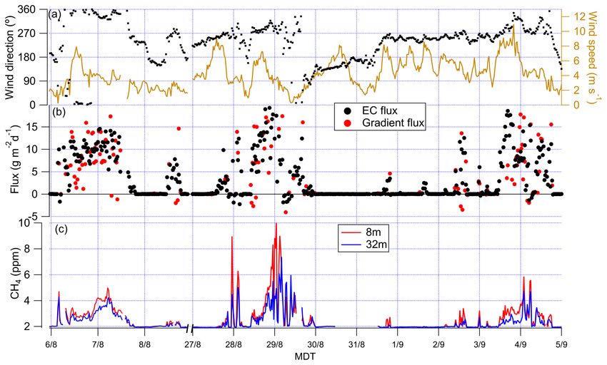
1880                                                          Y. You et al.: Methane emissions from an oil sands tailings pond

radiative forcing to the total of 2.83 W m−2 by all well-mixed      32 m) above ground plus another sampling level at 4 m above
greenhouse gases since the beginning of the industrial era          ground on the roof of the trailer housing the instruments. This
(Myhre et al., 2013). CH4 can be produced by microbes in            setup allowed the measurement of the vertical gradient of
the oil sands tailings through methanogenic degradation of          gaseous pollutant concentrations and meteorological condi-
hydrocarbon in diluents and unrecovered bitumen (Siddique           tions. Gas inlets at these levels were connected to a range of
et al., 2007, 2011, 2012; Penner and Foght, 2010; Foght et          instruments in the trailer located right beside the flux tower,
al., 2017; Kong et al., 2019).                                      through 40 m of 1/2 in. (1.27 cm) outer diameter Teflon tub-
   Most commonly, flux chambers have been used to deter-            ing for the upper three levels and 7 m of tubing for the low-
mine the emission rate of GHGs from tailings ponds (Small           est level. For the gradient measurements, a cavity ring-down
et al., 2015; Stantec, 2016). These chambers cover an area          spectroscopy instrument (Picarro, model G2204) was used
of less than 1 m2 each and result in only short snapshots of        to measure CH4 and hydrogen sulfide (H2 S) at four levels by
emissions that may not capture the spatiotemporal variabil-         cycling through the levels every 10 min (i.e., 2.5 min at each
ity of emissions. Tailings ponds in the oil sands region typi-      level). Readings from the first 30 s after each level switch
cally have a size of 0.1–10 km2 with heterogeneous surfaces.        were discarded.
Micrometeorological methods of determining fluxes, such as             For the EC measurements, another cavity ring-down spec-
eddy covariance (EC) (Foken et al., 2012) and gradient fluxes       troscopy (CRDS) instrument (Picarro, model G2311f) was
(Meyers et al., 1996), are non-intrusive and continuous meth-       used to measure the mole fraction of CH4 , CO2 , and H2 O
ods that can be used to measure fluxes from area sources.           (water vapor) at 10 Hz. It sampled from the 18 m level
These methods intrinsically produce integrated flux estimates       through a 30 m 3/8 in. outer diameter Teflon tube at a flow
representative of hectares to km2 . In addition, inverse disper-    rate of 7 L min−1 .
sion models (IDMs) (Flesch et al., 1995) and vertical radial           Calibrations of CH4 for all the CRDS instruments were
plume mapping (VRPM) (Hashmonay et al., 2001) can be                performed before and after the field project against secondary
used to combine micrometeorological information with mea-           standards traceable to standards used by Environment and
sured pollutant concentrations to deduce surface–atmosphere         Climate Change Canada (ECCC) for their GHG observa-
exchange rates.                                                     tional program, which are in turn traceable to World Mete-
   Micrometeorological methods applied to large areas of a          orological Organization (WMO) standards.
tailings pond can provide much needed information on the               At each of the three levels on the tower, an ultrasonic
spatial and temporal variabilities of emission fluxes from tail-    anemometer (Campbell Scientific, model CSAT3) measured
ings ponds as an input for air quality and climate change           the turbulent motions in the atmosphere, i.e., u, v, w (the
modeling. Tailings ponds represent a useful testing ground          three orthogonal components of the wind) and T (sonic tem-
for a multi-method comparison of flux measurement tech-             perature), at 10 Hz. The momentum flux and the sensible
niques due to their reliability as sources of significant fluxes,   heat flux can be calculated from the covariance of the ver-
relatively well defined sources areas, and minimal other an-        tical wind component with horizontal wind and temperature
thropogenic sources in the immediate vicinity. This paper de-       fluctuations, respectively, through EC. Friction velocity (u∗ )
scribes the results of a comparison of flux chambers, EC, gra-      can also be calculated from measured u, v, and w (u∗ =
                                                                           2        2
dient, and IDM approaches for estimating emission rates of          (u0 w 0 + v 0 w0 )1/4 ). The two lower ultrasonic anemometers
CH4 , to verify the suitability of these methods for quantify-      pointed towards true north, whereas the ultrasonic anemome-
ing fugitive emissions from such sources.                           ter at 32 m pointed at 3.5◦ . An adjustment to the true north
                                                                    was applied during analysis. There was also a propeller
                                                                    anemometer (Campbell, model 05103-10) on the trailer roof
2   Site and measurement description                                4 m above ground, measuring wind speed and direction. Am-
                                                                    bient temperature and relative humidity (RH) were measured
The main site of this study was on the south shore of               with sensors at three levels on the tower and 1 m above
Suncor Pond 2/3 (Fig. 1; 56◦ 590 0.9000 N, 111◦ 300 30.3000 W;      ground (Rotronic, model HC2-S3-L; shield: Campbell Sci-
305 m a.s.l.). The Suncor main facility was 2.6 km to the           entific, model 43502). Ambient pressure was measured with
northeast, and the Syncrude main facility was 9 km to the           a barometer (RM Young model 61202). A net radiometer
northwest. The pond liquid surface area was about 2.5 km by         (Kipp & Zonen, model CNR1) was used to measure solar
1.3 km. Within 2 km to the south of our measurement site,           radiation during the entire project. An infrared remote sensor
the landscape included natural landscapes, a workers camp,          (Campbell Scientific, model SI-111) was mounted at 32 m on
and parking lots. There were also other facilities and sources      the tower looking down at an angle of 30◦ below the horizon-
around the pond, but they were too far from our measurement         tal to measure the temperature at the pond surface. With an
site to contribute to the fluxes measured using the methods in      angular field of view of 44◦ , this results in a footprint ranging
this study (Sect. 4.2). Measurements were conducted from            from 25 to 228 m from the tower. Given the location of the
28 July to 5 September 2017. The sampling platform was
a 32 m mobile tower instrumented at three levels (8, 18, and

Atmos. Meas. Tech., 14, 1879–1892, 2021                                               https://doi.org/10.5194/amt-14-1879-2021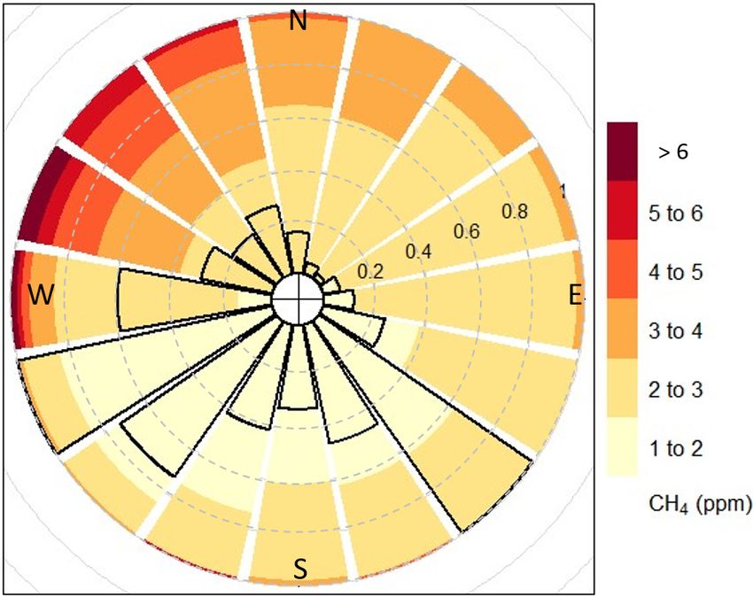
Y. You et al.: Methane emissions from an oil sands tailings pond 1881
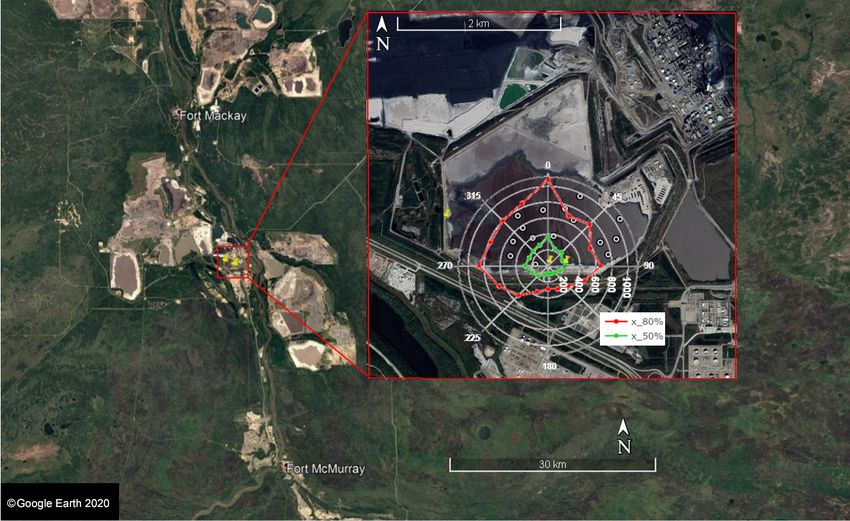
Figure 1. Overall map of the study site and close-up of the pond in September 2017. The superimposed polar plot shows the footprints under
unstable conditions. Two traces in the polar plot show the medians of 80 % and 50 % contribution distances (in meters) for the measured
half-hour EC fluxes in 16 wind direction bins. Angles in the polar plot are the wind direction (true north) with the center at the main site. The
15 white circles on the surface of the pond indicate the locations of the flux chamber measurements. The gray areas north of the r = 1100 m
circle are sandy deposits; dark gray represents liquid surfaces.
tower relative to the pond, winds from between 286 and 76◦ 3 Methods for deriving fluxes
were defined as coming from the pond (Fig. 1).
An open-path Fourier transform infrared (OP-FTIR) spec- 3.1 Eddy covariance flux
trometer system (Open Path Air Monitoring System (OPS),
Bruker) was set up at the site to measure line-integrated mole EC fluxes represent a direct measurement of the turbulent
fractions of CH4 and other pollutants. The spectrometer was vertical exchange of a substance and as such usually serve
set up in a trailer next to the main tower about 1.7 m above the as a reference (Foken et al., 2012) to which more indirect
ground, pointing to three retro-reflectors 200 m to the east. methods (such as those described below) can be compared
The lowest retro-reflector was on a tripod, and the higher two (Bolinius et al., 2016; Prajapati and Santos, 2018). EC typ-
retro-reflectors were supported by JLG basket lifts, resulting ically requires fast response time measurements (on the or-
in heights of the three retro-reflectors of approximately 1.7, der of 0.1 s) and high sampling frequency (> 5 Hz) (Foken et
11, and 23 m above ground. The spectrometer automatically al., 2012), which in this study limits the method to sensible
cycled through pointing at these three sequentially. Spectra and latent heat (H2 O) fluxes, momentum, and CO2 and CH4
were measured at a resolution of 0.5 cm−1 with 250 scans fluxes.
co-added, resulting in roughly 1 min resolution. Other details As summarized in Foken et al. (2012), in the EC method,
on the OP-FTIR setup and spectral retrieval analysis can be flux is calculated by averaging the product of the deviations
found in You et al. (2021). of the vertical wind component and a mole fraction from their
means. For compound c and vertical wind component w, the
flux Fc is thus
Fc (EC) = w0 c0 , (1)
where the mole fraction c = c +c0 , with the overbar denoting
the average and the prime a deviation from it, and similarly
https://doi.org/10.5194/amt-14-1879-2021 Atmos. Meas. Tech., 14, 1879–1892, 2021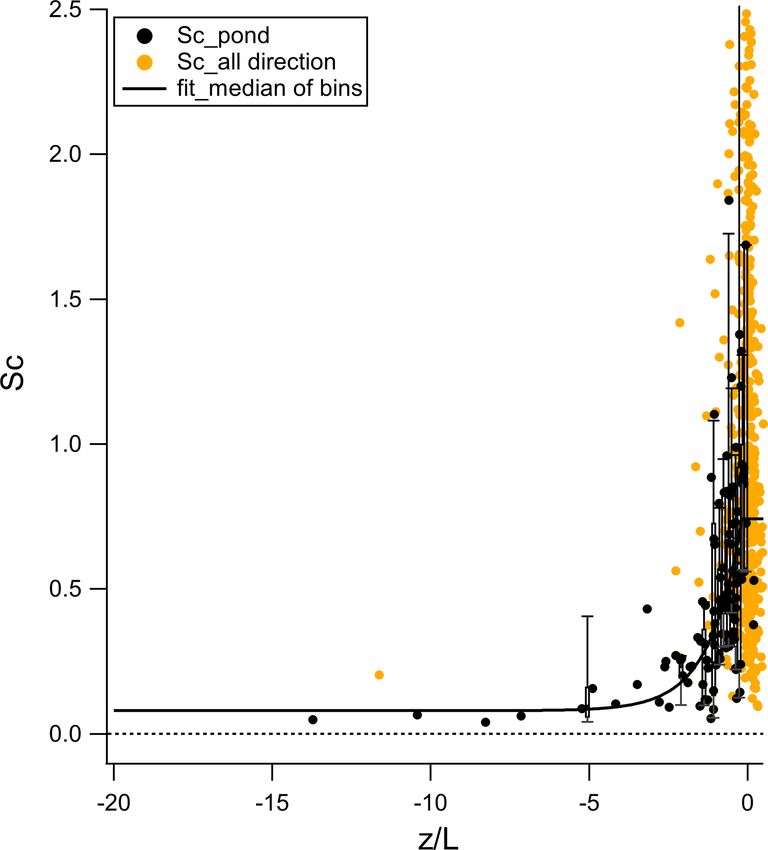
1882                                                           Y. You et al.: Methane emissions from an oil sands tailings pond

for w. To account for “storage”, i.e., the vertical buildup or       (Stull, 2003a). The flux is then given by
venting of a gas between the source and the measurement                            ∂c
level (assuming a linear vertical profile of gas concentration),     Fc = −Kc         ,                                           (3)
                                                                                   ∂z
a storage term is added, so that the total flux is given by
                                                                     where Fc is the gradient flux for a pollutant c, and ∂c∂z is the
               Zz
                    ∂c                                               vertical mole fraction gradient. Note that in this notation, Kc
Fc = w0 c0 +           ∂z.                                    (2)    incorporates any stability corrections required since stabil-
                    ∂t
               0                                                     ity effects on the relationship between vertical mole fraction
   In this study, 30 min averages of the EC flux of CH4              gradients and turbulent fluxes are already incorporated. Our
were calculated by combining the 18 m CRDS CH4 data                  approach follows the well-established modified Bowen ratio
with the CSAT measurements. The raw data were processed              (MBR) method (Meyers et al., 1996; Bolinius et al., 2016).
by EddyPro (version 6.0.0, LI-COR Inc.), and major pro-              To calculate Kc of CH4 , the measurements of CH4 EC flux
cesses included axis rotation (double rotation) (cf. Wilczak,        and a gradient of mole fraction are required by Eq. (3). From
et al., 2001), time lag compensation (covariance maximiza-           the measurements at the 18 m, we have a direct EC flux for
tion method) (Fan, et al., 1990), and storage term correction        CH4 . Since the footprint of fluxes derived from mole fraction
(Foken et al., 2012). The time lag on average was 10.5 s. Co-        gradients between 8 and 32 m is approximately equivalent to
variance spectra were examined for signal losses at higher           the EC footprint at 18 m (see discussion in Sect. 4.2), this
frequencies (smaller eddies) during transit of the sampled           gradient can be combined with the EC flux to calculate Kc
air through the sample line, finite sample cell volume, and          by Eq. (3). However, only a fraction of the observations yield
instrument response (Fig. S1 in the Supplement), account-            well-resolved CH4 fluxes and gradients, whereas a continu-
ing for a loss of typically 15 % of covariance signal com-           ous time series of Km , the eddy diffusivity for momentum
pared to the sensible heat cospectrum that does not suf-             (wind speed) by Eq. (4) (Stull, 2003a), can be readily es-
fer from equivalent losses. Spectral corrections following           tablished. Therefore, we establish a relationship between Kc
Horst (1997) were applied to correct for these losses. Correc-       and Km for those periods when this is feasible and calculate
tions for signal losses at the low-frequency end of the spectral     the ratio of these two, which by definition is the so-called
peak due to the finite averaging time were applied according         “Schmidt number” in Eq. (5) (Gualtieri et al., 2017),
to Moncrieff et al. (2004). The EC flux quality flag was cate-                      ∂u
gorized into three classes: 0 (best quality), 1 (good quality),      Fm = −Km          ,                                          (4)
                                                                                    ∂z
and 2 (poor quality) (Mauder et al., 2006; Mauder and Fo-                   Km
ken, 2004). Only EC fluxes with flag 0 or 1 were included in         Sc =      .                                                  (5)
                                                                            Kc
further analysis.
   Although the slope of the shoreline of the pond was very             To get the Schmidt number Sc by Eq. (5), two approaches
gentle and the wind was not expected to experience any sig-          were used: the first approach is with a constant Sc. A lin-
nificant perturbations near the flux tower, we also tested cal-      ear regression of binned Kc versus Km bins was performed.
culating the CH4 EC flux using a sector-wise planar-fit coor-        The inverse of this slope (Fig. 2), as defined in Eq. (5), is the
dinate rotation (Wilczak et al.,2001). Four sectors were de-         Schmidt number. The least-squares fit produces a Sc = 0.74,
fined: 286–76◦ (pond sector); 76–124◦ (east shoreline sec-           which falls between published values of 0.99 by Gualtieri et
tor), 124–259◦ (the south sector); 259–286◦ (west shoreline          al. (2017) and the average value of 0.6 in Flesch et al. (2002).
sector). The resulting half-hour CH4 EC flux and the flux us-        Since due to the intermittent nature of CH4 a measured Kc is
ing double rotation were within 0.0 ± 0.1 g m−2 d−1 of each          only available a fraction of the time, we use the more con-
other (mean and SD of the difference). Therefore, as ex-             tinuous momentum eddy diffusivity Km divided by Sc as our
pected, during this campaign at this site the planar fitting         Kc .
method did not significantly change the final CH4 EC flux               The second approach is with variable Sc. Gualtieri et
results.                                                             al.(2017) reviewed experimental and numerical simulation
                                                                     studies of the turbulent Schmidt number in the atmospheric
3.2    Gradient flux method                                          environment and reported Sc values from 0.1 to 1.3. Flesch et
                                                                     al. (2002) measured the turbulent Sc of a pesticide in the at-
Gradient flux estimates are based on relationships between           mosphere from soil emissions. Reported Sc in that study var-
the vertical gradient of mole fractions and the associated flux      ied from 0.17 to 1.34 and showed that this was not solely due
(down the gradient from high to low mole fractions). In the          to measurement uncertainty. The Sc in this study also varies
atmosphere, turbulent exchange dominates molecular diffu-            significantly over time when the wind is from the pond, from
sion by several orders of magnitude under most conditions,           0.04 to 2.90.
and the factor relating the gradient to the flux is a transfer co-      To investigate the real variability in Sc, Sc =
efficient dependent on the characteristics of turbulence (first-     Km_measured /Kc_measured was plotted against the stabil-
order closure, K-theory), called the eddy diffusivity (Kc )          ity parameter z/L (Stull, 2003b), where L is the Obukhov

Atmos. Meas. Tech., 14, 1879–1892, 2021                                                    https://doi.org/10.5194/amt-14-1879-2021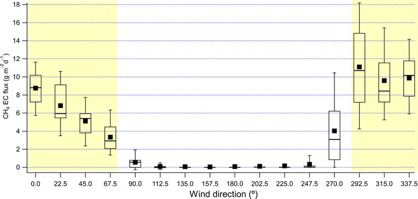
Y. You et al.: Methane emissions from an oil sands tailings pond 1883
Figure 2. Calculating the Schmidt number Sc as a constant over the
entire study. Lower and upper bounds of the box are the 25th and
Figure 3. Dependence of Sc on z/L measured at 18 m. Yellow
75th percentile of each bin; the lines in the box and the blue squares
points are Sc observed in each individual half-hour period over the
mark the median; the red circle labels the mean of the data in each
entire period; black points are Sc observed in each individual half-
bin; whiskers are the 10th and 90th percentile of the data. In this
hour period when the wind was from the pond; the black curve is
analysis, measured Kc values were binned by Km with 65 points in
the best fit of Sc versus median z/L from each z/L bin when the
each bin. Bin centers were the median Km measured of each bin.
wind was from the pond. In this analysis, Sc was binned by z/L
The red line is the best fit of mean Kc vs. median Km of each bin.
with 10 points in each bin before fitting.
The p value of the fit = 0.0001. Points with Km > 5 m2 s−1 were
excluded in the fit.
results with the constant Sc approach are shown in Table S1
length, for periods when the wind was from the pond in the Supplement for comparison.
direction (Fig. 3). Figure 3 shows that Sc becomes small as It is possible to calculate Kc values based on CO2 in or-
z/L indicates increasingly unstable turbulent mixing, i.e., an der to avoid potential circularity arguments when calculat-
increasing importance of convective (sensible heat driven) ing gradient fluxes of CH4 using this approach. However,
turbulence, which is not captured by an uncorrected Km , vs. the CO2 flux signal from this pond was confounded by the
mechanical (momentum driven) turbulence. Sc varies sig- strong natural variability of the CO2 background, as well as
nificantly with z/L and is associated with significant noise the smaller signal-to-noise ratio of the pond CO2 flux com-
near neutral stability (z/L close to 0). To avoid introducing pared to the CH4 flux (Fig. S1). Regardless, Kc values based
large scatter in the Sc correction near neutral stability, Sc is on CO2 were calculated and found to be noisier but statisti-
set as 0.74 when z/L is close to 0. To make the correction cally not different from those based on CH4 (t test p = 0.09,
function continuous, a stepwise definition for Sc is given: based on fluxes binned into 16 wind direction sectors). It
would also be possible to base the calculated Kc values on
z the sensible heat flux instead of the momentum flux, but due
L +19.5
1.008
z
Sc = 0.08 + 3.13 × 10⁻⁹ e , L < −0.18 (6) to the absence of significant heat fluxes at night, this would
0.74, z
≥ −0.18. not provide the continuity that the momentum fluxes afford.
L
3.3 Inverse dispersion fluxes
This Sc of the entire study period and a time series of Kc =
Km /Sc (corresponding to 8 and 32 m measurements) were Inverse dispersion models (IDMs) can be used to derive
calculated. A three-point median smoothing was performed emission rate estimates based on line-integrated or point
with the calculated Kc time series before the gradient flux mole fraction measurements downwind of a defined source.
of CH4 was calculated using Eq. (3). To lessen the impact Required inputs include the turbulence statistics between the
of extreme outliers, the final pond average fluxes reported source and point of observation. Unlike the EC and gradi-
were based on gradient fluxes between the 2.5th and 97.5th ent techniques, IDMs also require an estimation of the back-
percentiles. In the Results and discussion section, gradient ground mole fraction of the pollutant upwind of the source.
fluxes and plots from the variable Sc approach are shown, and The backward Lagrangian stochastic (bLS) models are a spe-
https://doi.org/10.5194/amt-14-1879-2021 Atmos. Meas. Tech., 14, 1879–1892, 2021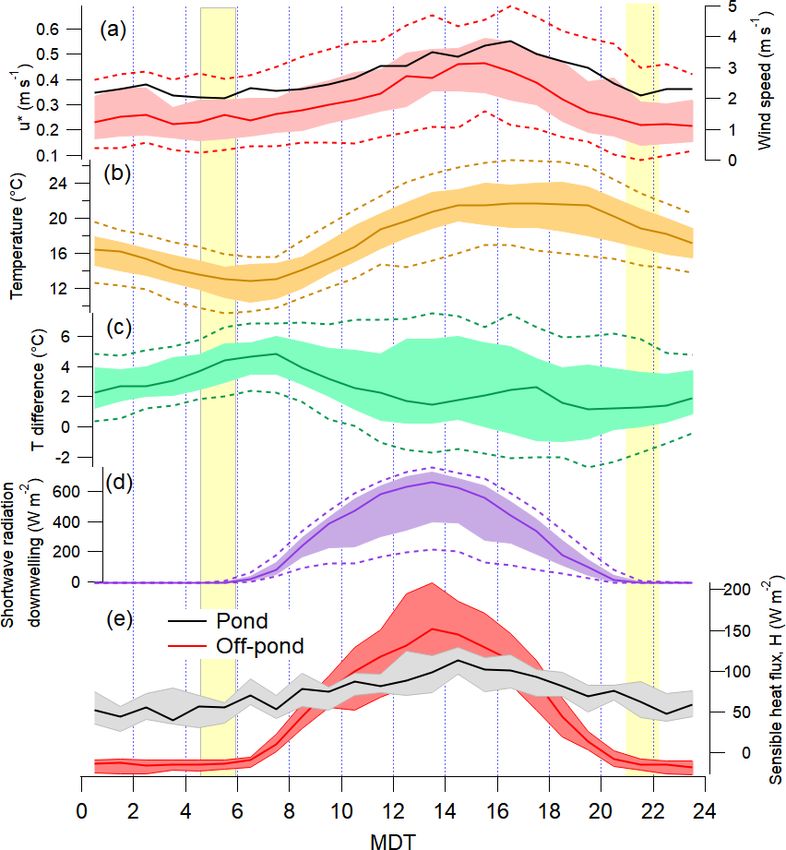
1884                                                        Y. You et al.: Methane emissions from an oil sands tailings pond

cific subtype of IDMs. WindTrax 2.0 (Thunder Beach Sci-           Table 1. Summary of CH4 fluxes (g m−2 d−1 ) in this study.
entific, http://www.thunderbeachscientific.com, last access:
26 January 2021; Flesch et al., 1995), based on a bLS model,          Flux method            Q_25 %          Median        Q_75 %             Meanc
is used in this study. The emission rate Q (g m−2 d−1 ) is cal-
                                                                      ECa                           5.6            7.4           9.8       7.8 ± 1.1
culated through
                                                                      Gradienta                     3.8            6.1          11.0       7.2 ± 3.5
                                                                      IDMa                          3.6            5.2           6.6       5.4 ± 0.4
   (C − Cb )                                                          Flux chamberb                 2.0            2.3           3.8       2.8 ± 1.4
Q=         ,                                             (7)
        C
        Q sim                                                      a Statistics and average fluxes are area weight averaged. b Statistics and average of
                                                                   15 measurements described in Sect. 4.6. The error of the mean is the SD of the
                                                                   15 measurements. Emission estimates were 5.3 g m−2 d−1 in 2016 and
where C [ppm] is the pollutant mole fraction at the measure-       11.1 g m−2 d−1 in 2018. c Errors with the mean fluxes are calculated with a
ment location, Cb is the background mole fraction of the pol-      top-down error estimation approach, using the average of SDs of fluxes from five
                                                                   periods when the fluxes displayed high stationarity.
lutant, and (C/Q)sim is the simulated ratio of the pollutant
mole fraction at the site to the emission rate from the spec-
ified source calculated by the bLS model. In this study, the      3.5    Area-weighted average of flux
meteorological condition inputs for the bLS model are u∗ and
L taken from the 30 min averaging calculation of ultrasonic       To derive fluxes representing the whole pond, the half-hour
anemometer measurements at 8 m, as well as 30 min aver-           fluxes (EC, gradient, and IDM fluxes) are binned by wind
age wind directions and ambient temperature directly from         direction into 16 sectors. Area-weighted averages of fluxes
the propeller and temperature sensor at 4 m. Periods when         for the pond Fpond are then calculated by
u∗ < 0.15 m s−1 were disregarded (Flesch et al., 2004). CH4
mole fraction input was taken from the OP-FTIR measure-
                                                                                P
                                                                                      F (flux, sector) · Area (sector)
ment, which was located 10 m to the east of the flux tower.       Fpond =
                                                                              sectors
                                                                                        P                              .                              (9)
Emission rates are calculated by IDM only when the wind                                    sectors Area (sector)
came from the pond, including the sectors centered at 270
and 90◦ .                                                            The area-weighted averages of flux results are summarized
                                                                  in Table 1 and serve as the final average fluxes representing
3.4    Flux chamber measurements                                  the whole pond over the study period.

Floating flux chamber measurements of CH4 and CO2 were
                                                                  4     Results and discussion
conducted at 15 spots in and around bubbling zones, includ-
ing 4 within 500 m of the tower, from 31 August to 2 Septem-      4.1    Meteorological conditions
ber 2017, by Barr Engineering Co., using compliance moni-
toring procedures established with guidance from the Quan-        As shown in the wind rose (Fig. S2 in the Supplement), wind
tification of Area Fugitive Emissions at Oil Sands issued by      coming from the pond occurred only about 22 % of the en-
Alberta Environment and Parks (AEP, 2019). On-site anal-          tire measurement period. The dominance of winds from the
ysis of GHG was performed using U.S. Environmental Pro-           background directions was known before the study, based
tection Agency (USEPA) flux chambers with real-time GHG           on records from monitoring stations in the area, but logis-
analyzers (Los Gatos Research, Inc., USA). These flux cham-       tical and access constraints limited us to using the south
ber measurements were conducted during daytime. Key pro-          shore for the setup. There was no significant diurnal varia-
cedural steps include 45 min of purging pure nitrogen gas to      tion in wind direction over the entire period. The ambient
reach an equilibrium between the flow of the inert carrier gas    temperature during the measurement period varied from 7.5
and the methane evolving from the pond surface, and mea-          to 31.1 ◦ C, with an average of 17.5 ◦ C (Fig. 4b). The mean
surement for a minimum of 30 min of with steady-state con-        wind speed measured with the propeller anemometer at 4 m
centration readings. GHG gases reported from the chamber          was 3.0 m s−1 , with a range from 0 to 14.9 m s−1 , and quar-
measurements include CH4 , CO2 , and N2 O (nitrous oxide).        tiles of 1.7 and 4.0 m s−1 (Fig. 4a). The mean friction velocity
Fluxes were calculated according to the USEPA user’s guide        at 8 m (the lowest height by sonic anemometer measurement)
EPA/600/8-86/008 (USEPA 1986, Eqs. 3–5):                          over the whole measurement period was 0.32 m s−1 (Fig. 4a),
                                                                  with a range from 0.03 to 1.01 m s−1 and quartiles are 0.20
             Q·C                                                  and 0.42 m s−1 . Wind speed and friction velocity had a pre-
Fchamber =       ,                                         (8)
              A                                                   dictable diurnal pattern: greater during the day than at night
                                                                  (Fig. 4a).
where Q is the flux chamber sweep air flow rate (L min−1 ),          In Fort McMurray during the study period, the sunrise
A is the enclosed surface area (m2 ), and C is measured con-      was in the range of 04:35 to 05:56 MDT (mountain day-
centration (µg L−1 ).                                             light savings time, UTC−6), solar noon occurs at around

Atmos. Meas. Tech., 14, 1879–1892, 2021                                                   https://doi.org/10.5194/amt-14-1879-2021
Y. You et al.: Methane emissions from an oil sands tailings pond 1885
sured at 18 m at each half-hour period were estimated us-
ing the algorithm by Kljun et al. (2015), which takes mean
wind speed, boundary layer height, wind direction, friction
velocity, Obukhov length, and SD of horizontal wind speed.
Boundary layer height was estimated using the lidar mea-
surements at Fort McKay in August 2017 (Strawbridge et
al., 2018). Footprints under unstable conditions are sum-
marized in the polar plot in Fig. 1. Footprint contribution
distances were calculated for each half hour over the en-
tire period of study. Results were further separated into un-
stable (z/L ≤ −0.0625), neutral (−0.0625 < z/L < 0.0625),
and stable (z/L ≥ 0.0625) conditions. Since unstable condi-
tions applied 98.6 % of time when the wind was from the
pond and 52 % of entire measurement period, we summa-
rized the unstable condition footprint results into 16 wind
direction bins, and medians are shown in the polar plot in
Fig. 1 (footprint under neutral and stable conditions is shown
in Fig. S3 in the Supplement). The footprint results show the
EC flux footprint lies mostly within the edges of the pond.
For gradient flux measurements, the effective footprint is
the same as the EC footprint at the geometric mean of the two
sample heights (Horst, 1999) for a homogeneous surface area
upwind. In this study, gradients between 8 and 32 m therefore
Figure 4. Diurnal variations of (a) u∗ at 8 m (red) and wind speed have a footprint equivalent to that for EC at 16 m, reasonably
at 4 m (black); (b) ambient temperature at 8 m; (c) the temperature close to where the 18 m EC fluxes were measured. Since the
difference between the surface of the pond and the ambient temper-
concentration footprint at the upper (32 m) level is larger than
ature at 8 m; (d) downwelling shortwave radiation; (e) the sensible
the concentration footprint at the lower (8 m) level, the gra-
heat flux at 8 m. Solid lines show the median, shades indicate the
interquartile ranges, and dashed lines label the 10th and 90th per- dient flux may be affected by sources beyond the geometric
centiles. MDT denotes mountain daylight savings time (hours). The mean footprint.
yellow shades mark the range of local sunrise and sunset times dur-
ing this 5-week project. 4.3 Eddy covariance flux
Analysis of CH4 mole fractions at 18 m as shown in Fig. 5
13:30 and sunset occurs in the range of 22:25 to 20:49 MDT clearly indicates that CH4 was elevated when the wind was
(Fig. 4d). Winds across the pond and from the south pass over from the pond direction, and it was steady at round 1.9 ppm
markedly different surface types (liquid pond vs. a mixture when the wind was from other directions (Figs. 5 and 6).
of solid surface types), so the sensible heat flux H is ana- Besides sectors from the pond directions, Fig. 7 shows CH4
lyzed separately based on the wind direction (Fig. 4e). Dur- fluxes significantly larger than zero from two sectors cen-
ing the day (from 08:00 to 19:00), H associated with winds tered with 90 and 270◦ , i.e., along the shorelines to the east
across the pond was consistently smaller than H with winds and west. Therefore, measured results for air coming from
from other directions, suggesting the pond absorbs signifi- these two sectors could represent a mixture of air carrying
cant solar energy at the site during the day. It is also worth pond emissions and air from the shore. EC fluxes from the
mentioning that H stayed positive during the night when the four wind direction sectors centered in the range of 292.5 to
wind came across the pond, consistent with the observation 0◦ are close to each other.
that the pond surface temperature was greater than the air There was no statistically significant diurnal pattern of the
temperature (Fig. 4c). These resulted in convective turbulent CH4 EC flux when the wind came from the pond direction
transport of species emitted from the pond surface through- (WD ≥ 286◦ or WD ≤ 76◦ ) (relative SD is 15 %, p = 0.54)
out the night. (Fig. S4a in the Supplement). The diurnal pattern of an-
other three sectors when the wind was not from the pond
4.2 Footprint of flux measurements were studied. The sector 259◦ ≤ WD < 286◦ (Fig. S4b) con-
tains a mixture of pond emission and the shore of the pond,
The footprint of a micrometeorological flux measurement, and it also showed no significant diurnal pattern. The sector
i.e., the area upwind that contributes to the flux at the point 214◦ ≤ WD < 259◦ (Fig. S4c) mainly covers trees and a lake
of observation, depends on the wind speed and the dynamic and showed a slightly increased flux during 12:00–18:00,
stability of the surface layer. The footprints of EC fluxes mea- which is likely due to biogenic emission from trees and
https://doi.org/10.5194/amt-14-1879-2021 Atmos. Meas. Tech., 14, 1879–1892, 20211886 Y. You et al.: Methane emissions from an oil sands tailings pond
the half-hour gradient fluxes were statistically different from
the EC fluxes when the wind was from the pond direction
(p = 0.003). They were moderately correlated (slope = 0.80,
r = 0.32, Fig. S7a in the Supplement). To obtain some com-
parability, it is therefore necessary to average blocks of data
into appropriate bins. A t test of the gradient and eddy av-
erage fluxes binned by wind direction (22.5◦ blocks) yielded
a p = 0.30, and hourly diurnal averaged fluxes agreed with
a p = 0.09. The pond-area-weighted mean gradient flux was
8 % lower than EC flux, and the median was 18 % less than
EC flux (Table 1).
Studies comparing MBR and EC CH4 fluxes are rare. Zhao
et al. (2019) compared CH4 fluxes from an MBR method as
well as from an aerodynamic flux model to EC fluxes for two
small fish ponds and showed that the MBR fluxes were well
correlated with EC fluxes, with a mean 27 % greater than the
Figure 5. Rose plot of CH4 mole fraction at 18 m. Colors represent EC mean flux. The gradient flux calculation in our study can
CH4 mole fraction. The length of each colored segment represents be considered a hybrid of the MBR and aerodynamic meth-
the time fraction of that mole fraction range in each direction bin. ods, based on a continuous time series of eddy diffusivities
The radius of the black open sectors indicates the frequency of wind for momentum, scaled by the eddy diffusivity for CH4 . The
in each direction bin; the angle represents wind direction. gradient fluxes of CH4 agreed well with EC flux in our study,
providing a basis for applying the derived Kc values to cal-
culate gradient fluxes for a variety of other gases emitted by
soils (Covey and Megonigal, 2019). The sector 124◦ ≤ WD the pond (e.g., You et al., 2021). Other studies comparing
< 146◦ (Fig. S4d) covered a workers’ lodge and parking lots, MBR with eddy covariance methods on other gases fluxes,
and CH4 emissions and diurnal variation were close to zero. such as CO2 , have been reported. Xiao et al. (2014) showed
The lack of a diurnal variation of CH4 EC flux observed that fluxes of CO2 from these two methods were comparable
when the wind was from the pond in this study was simi- at Lake Taihu. Wolf et al. (2008) and Bolinius et al. (2016)
lar to the lack of diurnal variation of CH4 EC flux at another used EC of heat to derive gradient fluxes of CO2 over trees
tailings pond reported by Zhang et al. (2019). and showed they were comparable with EC fluxes.
Relationships between the flux when the wind was from Gradient fluxes were also calculated with the constant Sc
the pond and various meteorological parameters were inves- approach, as described in Sect. 3.2, and results are listed
tigated, and results show that fluxes showed a weak depen- in Table S1. Gradient fluxes calculated from a constant Sc
dence on wind speed, u∗ , water surface temperature, or the were significantly lower than gradient fluxes with the vari-
temperature difference between the water surface and 8 m able Sc approach (p < 10−21 ; the pond average mean (me-
(Fig. S5 in the Supplement); i.e., they were not major drivers dian) is 33 % (34 %) lower, respectively). Results from this
of the CH4 emission rate. CH4 at this site is mainly produced study clearly present the variable nature of Sc and that cor-
through the methanogenesis of hydrocarbon by the microbes recting Sc with stability (z/L) is effective to improve gradi-
in the fine tailings covering a range of depth in the pond ent flux calculations. While the function derived (Eq. 6) is
(Penner and Foght, 2010; Siddique et al., 2011, 2012) and primarily a function of the characteristics of atmospheric tur-
therefore is not directly affected much by the meteorological bulence and should have broad applicability, it is based on
conditions at the surface or above the pond. a limited data set and should be verified in other settings in
future studies.
4.4 CH4 gradient flux and comparison with EC flux
4.5 CH4 inverse dispersion flux and comparison with
The CH4 mole fraction measured at 8 and 32 m shows that EC flux
winds across the pond carried significantly more CH4 than
from other directions, and there was a clear vertical gradient Compared to point measurements, path-integrated measure-
with mole fraction at 8 m on the order of 0.5 ppm or more ments have the advantage of being less sensitive to changes
higher than at 32 m (Fig. 6). Gradient fluxes were calculated in wind direction and being representative of larger areal
for all periods when valid EC fluxes and concentration gra- averages (Flesch et al., 2004). Therefore, the bottom path-
dients were available. The gradient flux derived from mea- integrated CH4 mole fraction of the FTIR was used as input
surements at 8 and 32 m shows that the flux was minimal for the IDM flux estimate. The bottom path measurement had
when the wind was from other directions, similar to the EC the greatest signal-to-noise ratio and a footprint on the order
flux (Fig. S6 in the Supplement). Due to significant scatter, of 1–2 km, which is comparable to the footprint of the EC and
Atmos. Meas. Tech., 14, 1879–1892, 2021 https://doi.org/10.5194/amt-14-1879-2021Y. You et al.: Methane emissions from an oil sands tailings pond 1887 Figure 6. Time series of (a) wind direction and wind speed, (b) CH4 EC fluxes and gradient fluxes, and (c) CH4 mole fractions at 8 and 32 m, from 6 to 9 August and from 27 August to 5 September. Figure 7. EC flux of CH4 as a function of wind direction binned in 22.5◦ bins. Lower and upper bounds of the box plot are the 25th and 75th percentile; the line in the box marks the median and the black square labels the mean; the whiskers label the 10th and 90th percentile. Yellow shades indicate the wind directions from the pond. gradient fluxes (Fig. 1). CH4 IDM flux calculated from the sectors similar to that described in Sect. 4.4 yielded agree- path-integrated mole fraction inputs from OP-FTIR bottom ment at the p = 0.08 level. The pond-area-weighted mean path measurements (when the OP-FTIR path was downwind IDM flux was 30 % smaller than EC flux, and the pond-area- of the pond) compared well to EC flux, based on the set of si- weighted median IDM flux was also 30 % smaller than EC multaneous half-hour periods when both EC and IDM fluxes median flux. Some of the differences are likely due to the were available. IDM and EC flux showed reasonable corre- different footprints of the two measurements. The footprint lation (r = 0.62) with a slope of 0.69 (Fig. S7b), although for turbulent fluxes is smaller than the footprint for concen- the averaged half-hour IDM fluxes are significantly different trations at the same height (Schmid, 1994). The IDM flux from EC fluxes (p < 10−4 ). Binning into 16 wind direction showed weak diurnal variations when the wind came from https://doi.org/10.5194/amt-14-1879-2021 Atmos. Meas. Tech., 14, 1879–1892, 2021
1888                                                        Y. You et al.: Methane emissions from an oil sands tailings pond

the pond directions (Fig. S8 in the Supplement), with smaller     was being overestimated by extrapolation from the cham-
fluxes during the day compared to fluxes at night (p = 0.04)      bers, which may have preferentially been located over bubble
– inconsistent with EC and gradient fluxes. As stated in          zones. Their EC fluxes were 2 orders of magnitude smaller
Sect. 3.3, half-hour periods when u∗ < 0.15 m s−1 were ex-        than CH4 flux in this study. Results from this study and
cluded in IDM calculation (Flesch et al., 2004). This filtering   Zhang et al. (2019) suggest that average tailings pond CH4
excluded more nighttime fluxes than daytime fluxes, which         emission extrapolated from a few individual flux chamber
caused more limited data in IDM nighttime fluxes and biased       measurements may significantly underestimate or overesti-
the t test.                                                       mate fluxes relative to area-averaging micrometeorological
   Since the background mole fraction input for IDM cal-          measurements.
culation could affect the flux estimates, two approaches to          This has also been shown over other water surfaces. Pod-
determining background mole fraction of CH4 for model             grajsek et al. (2014) investigated CH4 fluxes at the lake
inputs were tested: the daily minimum of CH4 from wind            Tämnaren and reported the fluxes from the EC and flux
sectors between 180 and 240◦ of OP-FTIR at our site; the          chamber were on the same order of magnitude. They stated
CH4 from another independent OP-FTIR measurement on               that due to the non-continuous measurement of flux cham-
the north shore of this pond (details are described in You et     bers, some high-flux short episodes could be missed. Schu-
al., 2021). Results of IDM fluxes with these two background       bert et al. (2012) measured CH4 fluxes from lake Rotsee
approaches agreed well (You et al., 2021).                        and reported the fluxes from the EC and flux chamber com-
                                                                  pared well. Erkkilä et al. (2018) measured CH4 flux at Lake
4.6    Flux chamber measurements                                  Kuivajärvi with the two methods when the lake was stratified
                                                                  and reported flux chamber measurements were significantly
Fluxes from the 15 flux chamber measurements over 3 d             greater than EC fluxes. In conclusion, while flux chambers
in and around the bubbling zones varied from 0.9 to               present advantages in terms of finer spatial and temporal res-
5.1 g m−2 d−1 , with an average of 2.8 g m−2 d−1 and a me-        olution for small sources or locations with high spatial het-
dian of 2.3 g m−2 d−1 . The average flux of the five measure-     erogeneity, reliance on a limited number of flux chamber
ments on the last day, 2 September, is 3.6 g m−2 d−1 , which      measurements can result in significant year-to-year variabil-
is the highest amongst the 3 d. The great variation amongst       ity, and spatially integrating methods such as eddy covari-
these 15 measurements shows the pond was highly heteroge-         ance or gradient fluxes will generally provide more represen-
neous in terms of CH4 emissions. The average fluxes from          tative averages.
these flux chamber measurements are about half of the aver-
age fluxes from the EC, gradient, and IDM methods. While          4.7   Comparison with previous results
the flux chamber measurements were deployed over the three
days, the wind was from the south, so no simultaneous com-        Emissions reported in Small et al. (2015) and a Stantec re-
parison could be made between flux chamber measurements           port (2016) (Table 2) represent estimates extrapolated from
and micrometeorological methods. However, based on the            individual flux chamber measurements and did not incorpo-
micrometeorological fluxes spanning more than a month,            rate any seasonal variations for microbial CH4 emissions.
there is no evidence of day-to-day variability of this mag-       Therefore, to compare result of this study to results summa-
nitude, and we conclude that the mismatch is due to spatial       rized in Small et al. (2015), we simply used 1 year = 365
or methodological differences.                                    equal days. Small et al. (2015) showed that CH4 emissions
   Annual compliance flux chamber measurements in 2016            from the same pond were 2.6 g m−2 d−1 based on the averag-
resulted in pond average fluxes of 5.3 and 11.1 g m−2 d−1 in      ing of flux chamber measurements during August to October
2018, despite similar operational parameters in these years as    in 2010 and 2011. A Stantec compliance report (2016) pre-
in 2017. We conclude that the underestimate in 2017 is not        sented flux chamber measurements on this pond with result-
an indication of a systematic bias of flux chambers but rather    ing average fluxes of 12.9 and 2.1 g m−2 d−1 (bubbling and
a measure of the uncertainty involved in flux estimates based     quiescent zones, respectively) in 2013 and 9.6 g m−2 d−1 and
on snapshot chamber measurements.                                 below the detection limit, respectively, in 2014. EC fluxes of
   A few other studies have also discussed differences            CH4 in this study are a factor of 2.8 greater than flux cham-
between flux chambers and micrometeorological methods             ber measurements which were taken during the last few days
(Schubert et al., 2012; Podgrajsek et al., 2014; Erkkilä et       of this project and a factor of 3 greater than emissions re-
al., 2018; Zhang et al., 2019). Zhang et al. (2019) measured      ported in Small et al. (2015). However, CH4 fluxes in this
CH4 emission from another tailings pond and reported flux         study are 19 % to 40 % smaller than the fluxes from the bub-
chamber measurements were more than 10 times greater than         bling zones in 2013 and 2014 (Stantec, 2016). The big differ-
fluxes from the EC method. They stated that strong erup-          ences between flux chamber measurements in the bubbling
tions of bubbles could overwhelm the chamber and result in        and quiescent zones may suggest micrometeorological mea-
a local underestimation of the flux. On the other hand, the       surements with a bigger footprint will perform better in quan-
lower EC flux estimate suggests that the area average flux        tifying emission from the whole pond. It is worth noting that

Atmos. Meas. Tech., 14, 1879–1892, 2021                                            https://doi.org/10.5194/amt-14-1879-2021
Y. You et al.: Methane emissions from an oil sands tailings pond 1889
Table 2. Comparison of CH4 fluxes (g m−2 d−1 ) in this study to previously reported fluxes.
TAPOS Small et al. Stantec report (2016) Baray et al. Flux chamber
(2017) (2015)a bubbling quiescent (2018)b (2017)
zones zones
CH4 7.8 (EC) 2.6 2013 12.9 2.1 17.1 2.8
2014 9.6 BDL
CO2 24.4 (EC) 16.4 2013 14.9 10.5 NA 21.2
2014 11.0 BDL
a The original units are t ha−1 yr−1 . Measurements were taken from August to October in 2010 or 2011. The pond area was
2.8 km2 as listed in Table 1 of Small et al. (2015). We assumed no seasonal variations to extrapolate from summer measurements
to annual totals. b The original number is 2.0 t h−1 , and the pond water surface area used was 2.8 km2 (Small et al., 2015).
BDL: below detection limit. NA: not available.
the seasonal variation of fugitive emission from tailings pond quential density inversion between oil layers and water in the
is still not well understood and that different daily emissions pond, FTT discharge diluent composition change, introduc-
are derived from the tabulated annual results from Small et tion of new materials and chemicals into the MFT, and conse-
al. (2015) depending on the annual extrapolation model used. quential change in microbial community (Small et al., 2015;
This reflects a general complication when comparing the 5- Foght et al., 2017). Natural lakes and wetlands emit at rates
week emission results in this study to annual emissions re- typically on the order of 0.005–0.05 g m−2 d−1 (Sanches et
ported in the past. al., 2019). Another independent approach to estimating CH4
Baray et al. (2018) calculated CH4 emission from this emissions is using an emission factor (EF) combined with
pond based on airborne measurement in 2013 over the whole diluent discharge rates to the pond. The EF was based on an
facility, combined with reported statistics stating that 58 % of MFT characterization and kinetics of methanogenesis for a
CH4 emissions within the facility were from tailings ponds, matured pond. Pond 2/3 is presumably similar in maturity
and 85 % of emissions from these tailings ponds were from and properties to the studied MFT in other oil sands facility
Pond 2/3. This resulted in an estimate of 2.0 ± 0.3 t h−1 , (Siddique et al., 2008). After incorporating the diluent loss
which converts to 17.1 g m−2 d−1 (for a pond area of 2.8 km2 , to the pond, the daily CH4 emissions were calculated and in-
Small et al., 2015, Table 2). This emission rate is significantly tegrated into an annual emission of 5860 t, which is compa-
(119 %) greater than emissions from the three micrometeoro- rable to annual emissions extrapolated from the micrometeo-
logical methods in this study, possibly because of the uncer- rological methods in this study. This approach requires some
tainties in the reported percentage contribution of CH4 emis- assumptions: first, that the kinetics of methanogenesis are a
sions from this pond to the whole facility. function of the maturity of the microbial community within
Suncor reported facility-wide emissions of CH4 for 2017 the target MFT; and, second, that the properties of the dilu-
of 5977 t (Government of Canada, 2017). The emissions ent feed stream remain constant over the period considered.
measured during the 5 weeks of this study extrapolated to This approach can provide emission estimates continually,
the year result in 6548 t yr−1 , i.e., 110 % of this total. This provided that the microbial state in the MFT and the dilu-
extrapolation assumes seasonal invariance of CH4 emissions ent discharge volumes and properties are tracked and remain
(e.g., January emissions are the same as August emissions) as consistent.
is common practice in monitoring reports (cf. Stantec, 2016). To put the CH4 emissions into a global warming context,
When comparing CH4 emissions in this study to emissions the CH4 fluxes can be combined with concurrent flux mea-
summarized in Table 2, it must be kept in mind that differ- surements of CO2 with the same instrumentation. Assuming
ent time periods are being compared and that several factors a GWP of CH4 = 28 (Myhre et al., 2013), the equivalent CO2
may contribute to variability of the emissions (Siddique et flux (FCO2eq ) from this tailings pond FCO2eq = FCO2 + (FCH4 ·
al., 2007, 2012). Pond 2/3 is an active pond, and the amount GWP) = 204 kt yr−1 , 90 % of which is due to CH4 . This ac-
and characteristics of input streams are variable with time. counts for only 3 % of Suncor’s facility CO2eq emissions in
Some of the facility-specific variables which could affect 2017 due to the dominance of other CO2 sources.
the methane emissions include the amount of diluent loss to
the pond, the proportions of diluent and hydrocarbons in the
froth treatment tailings (FTT) that enter matured fine tailings
5 Conclusions
(MFT) layers in the pond, density of microbes in the MFT,
physical disturbance of the MFT layers, transferring activi-
Results in this study have provided several estimates of the
ties of the MFT, pond water temperature change and conse-
emission of CH4 from this tailings pond using EC, gradi-
https://doi.org/10.5194/amt-14-1879-2021 Atmos. Meas. Tech., 14, 1879–1892, 20211890 Y. You et al.: Methane emissions from an oil sands tailings pond
ent, and IDM for a period of 5 weeks. The gradient and in- Financial support. This research has been supported by the Oil
verse dispersion methods agreed moderately with EC results Sands Monitoring Program, the Program for Energy Research and
(18 % and 30 % lower, respectively), which lends confidence Development (Natural Resources Canada), and the Climate Change
that the former two methods can provide valid flux estimates and Air Pollution Program (ECCC).
for other gases emanating from the pond. These results were
also compared to flux chamber measurements at this pond
taken during the study, showing flux chamber estimates were Review statement. This paper was edited by Huilin Chen and re-
viewed by Kukka-Maaria Kohonen and one anonymous referee.
64 % lower than those from micrometeorological methods.
The better agreement between the three micrometeorologi-
cal measurements flux results suggests that the larger foot-
print of micrometeorological measurements results in more
robust emission estimates representing most of the pond area. References
Fluxes were shown to have only a minor diurnal cycle, with
a 15 % variability, during the period of this study. To investi- Alberta Environment and Parks: Quantification of area fugitive
gate seasonal patterns, further studies measuring CH4 fluxes emissions at oil sands mines, available at: https://open.alberta.
ca/publications/9781460145814 (last access: 17 October 2020),
using micrometeorological methods at this pond or other tail-
2019.
ings ponds throughout the year are recommended. Baray, S., Darlington, A., Gordon, M., Hayden, K. L., Leithead,
A., Li, S.-M., Liu, P. S. K., Mittermeier, R. L., Moussa, S. G.,
O’Brien, J., Staebler, R., Wolde, M., Worthy, D., and McLaren,
Data availability. All data are publicly available at R.: Quantification of methane sources in the Athabasca Oil
http://data.ec.gc.ca/data/air/monitor/source-emissions-monitoring- Sands Region of Alberta by aircraft mass balance, Atmos.
oil-sands-region/emissions-from-tailings-ponds-to-the- Chem. Phys., 18, 7361–7378, https://doi.org/10.5194/acp-18-
atmosphere-oil-sands-region/ (Environment and Climate Change 7361-2018, 2018.
Canada, 2021). Bari, M. A. and Kindzierski, W. B.: Ambient volatile
organic compounds (VOCs) in communities of the
Athabasca oil sands region: Sources and screening
Supplement. The supplement related to this article is available on- health risk assessment, Environ. Pollut., 235, 602–614,
line at: https://doi.org/10.5194/amt-14-1879-2021-supplement. https://doi.org/10.1016/j.envpol.2017.12.065, 2018.
Bolinius, D. J., Jahnke, A., and MacLeod, M.: Comparison of
eddy covariance and modified Bowen ratio methods for mea-
Author contributions. YY and RS conducted the research and suring gas fluxes and implications for measuring fluxes of per-
wrote the manuscript; SGM contributed flux analysis and editing; sistent organic pollutants, Atmos. Chem. Phys., 16, 5315–5322,
RM contributed CH4 data; JB contributed operational data on the https://doi.org/10.5194/acp-16-5315-2016, 2016.
pond and contributed to the writing. Covey, K. R. and Megonigal, J. P.: Methane production and
emissions in trees and forests, New Phytol., 222, 35–51,
https://doi.org/10.1111/nph.15624, 2019.
Competing interests. James Beck is an employee of Suncor Energy. Environment and Climate Change Canada: Emissions from
The other authors have no competing interests. tailings ponds to the atmosphere, oil sands region, avail-
abl at: http://data.ec.gc.ca/data/air/monitor/source-emissions-
monitoring- oil-sands-region/emissions-from-tailings-ponds-to-
the-atmosphere-oil-sands-region/, last access: 26 January 2021.
Acknowledgements. The authors thank the technical team of An-
Erkkilä, K.-M., Ojala, A., Bastviken, D., Biermann, T., Heiska-
drew Sheppard, Roman Tiuliugenev, Raymon Atienza, and Raj
nen, J. J., Lindroth, A., Peltola, O., Rantakari, M., Vesala, T.,
Santhaneswaran for their invaluable contributions throughout; Julie
and Mammarella, I.: Methane and carbon dioxide fluxes over
Narayan for spatial analysis; Stewart Cober for management; and
a lake: comparison between eddy covariance, floating cham-
Stoyka Netcheva for home base logistical support. We thank Sun-
bers and boundary layer method, Biogeosciences, 15, 429–445,
cor and its project team (Dan Burt et al.), AECOM (April Kliachik,
https://doi.org/10.5194/bg-15-429-2018, 2018.
Peter Tkalec), and SGS (Nathan Grey, Ardan Ross) for site logistics
Fan, S. M., Wofsy, S. C., Bakwin, P. S., Jacob, D. J. and Fitzjar-
support.
rald, D. R.: Atmosphere-biosphere exchange of CO2 and O3 in
This work was partially funded under the Oil Sands Monitor-
the Central Amazon Forest, J. Geophys. Res., 95, 16851–16864,
ing Program and is a contribution to the program but does not nec-
1990.
essarily reflect the position of the program. We also acknowledge
Flesch, T. K., Wilson, J. D., and Yee, E.: Backward-time Lagrangian
funding from the Program of Energy Research and Development
stochastic dispersion models and their application to estimate
(NRCan) and from the Climate Change and Air Quality Program
gaseous emissions, J. Appl. Meteorol., 34, 1320–1332, 1995.
(ECCC).
Flesch, T. K., Prueger, J. H., and Hatfield, J. L.: Turbulent
Schmidt number from a tracer experiment, Agr. Forest Meteorol.,
111, 299–307, https://doi.org/10.1016/S0168-1923(02)00025-4,
2002.
Atmos. Meas. Tech., 14, 1879–1892, 2021 https://doi.org/10.5194/amt-14-1879-2021Y. You et al.: Methane emissions from an oil sands tailings pond 1891
Flesch, T. K., Wilson, J. D., Harper, L. A., Crenna, B. P., and Sharpe, Liggio, J., Li, S. M., Hayden, K., Taha, Y. M., Stroud, C., Darling-
R. R.: Deducing ground-to-air emissions from observed trace gas ton, A., Drollette, B. D., Gordon, M., Lee, P., Liu, P., Leithead,
concentrations: A field trial, J. Appl. Meteorol., 43, 487–502, A., Moussa, S. G., Wang, D., O’Brien, J., Mittermeier, R. L.,
2004. Brook, J. R., Lu, G., Staebler, R. M., Han, Y., Tokarek, T. W.,
Foght, J. M., Gieg, L. M., and Siddique, T.: The microbiology of oil Osthoff, H. D., Makar, P. A., Zhang, J., Plata, D. L., and Liggio,
sands tailings: Past, present, future, FEMS Microbiol. Ecol., 93, J., Li, S. M., Hayden, K., Taha, Y. M., Stroud, C., Darlington,
fix034, https://doi.org/10.1093/femsec/fix034, 2017. A., Drollette, B. D., Gordon, M., Lee, P., Liu, P., Leithead, A.,
Foken, T., Aubinet, M., and Leuning, R.: Eddy Covariance: A Moussa, S. G., Wang, D., O’Brien, J., Mittermeier, R. L., Brook,
practical guide to measurement and data analysis, Eddy covari- J. R., Lu, G., Staebler, R. M., Han, Y., Tokarek, T. W., Osthoff, H.
ance method, edited by: Aubinet, M., Vesala, T., and Papale., D., Makar, P. A., Zhang, J., Plata, D. L., and Gentner, D. R.: Oil
D., Springer, 438 pp., https://doi.org/10.1007/978-94-007-2351- sands operations as a large source of secondary organic aerosols,
1, 2012. Nature, 534, 91–94, https://doi.org/10.1038/nature17646, 2016.
Galarneau, E., Hollebone, B. P., Yang, Z., and Schuster, J.: Liggio, J., Moussa, S. G., Wentzell, J., Darlington, A., Liu, P., Leit-
Preliminary measurement-based estimates of PAH emissions head, A., Hayden, K., O’Brien, J., Mittermeier, R. L., Staebler,
from oil sands tailings ponds, Atmos. Environ., 97, 332–335, R., Wolde, M., and Li, S.-M.: Understanding the primary emis-
https://doi.org/10.1016/j.atmosenv.2014.08.038, 2014. sions and secondary formation of gaseous organic acids in the
Government of Alberta: Specified gas reporting standard. oil sands region of Alberta, Canada, Atmos. Chem. Phys., 17,
2019 Version 11.0, available at: https://open.alberta. 8411–8427, https://doi.org/10.5194/acp-17-8411-2017, 2017.
ca/dataset/c5471471-79a3-456b-a183-997692da2576/ Liggio, J., Li, S. M., Staebler, R. M., Hayden, K., Darling-
resource/14073f8c-deab-410e-a9ab-ed326e5e4052/download/ ton, A., Mittermeier, R. L., O’Brien, J., McLaren, R., Wolde,
specified-gas-reporting-standard-v-11.pdf, last access: 21 Octo- M., Worthy, D., and Vogel, F.: Measured Canadian oil sands
ber 2019. CO2 emissions are higher than estimates made using inter-
Government of Canada: Greenhouse Gas Reporting Program, avail- nationally recommended methods, Nat. Commun., 10, 1863,
able at: https://climate-change.canada.ca/facility-emissions/ https://doi.org/10.1038/s41467-019-09714-9, 2019.
GHGRP-G10558-2017.html (last access: 4 December 2019), Mauder, M. and Foken, T.: Documentation and instruction manual
2017. of the eddy covariance software package TK2, available at: https:
Gualtieri, C., Angeloudis, A., Bombardelli, F., Jha, S., //core.ac.uk/download/pdf/33806389.pdf (last access: 24 Febru-
and Stoesser, T.: On the Values for the Turbulent ary 2021), 2004.
Schmidt Number in Environmental Flows, Fluids, 2, 17, Mauder, M., Liebethan, C., Göckede, M., Leps, J-P, Beyrich, F.,
https://doi.org/10.3390/fluids2020017, 2017. and Foken, T.: Processing and quality control of flux data
Hashmonay, R. A., Natschke, D. F., Wagoner, K., Harris, D. B., during LITFASS-2003, Bound.-Lay. Meteorol., 121, 67–88,
Thompson, E. L., and Yost, M. G.: Field evaluation of a method https://doi.org/10.1007/s10546-006-9094-0, 2006.
for estimating gaseous fluxes from area sources using open-path Meyers, T. P., Hall, M. E., Lindberg, S. E., and Kim, K.: Use of the
fourier transform infrared, Environ. Sci. Technol., 35, 2309– modified Bowen-ratio technique to measure fluxes of trace gases,
2313, https://doi.org/10.1021/es0017108, 2001. Atmos. Environ., 30, 3321–3329, https://doi.org/10.1016/1352-
Horst, T. W: A simple formula for attenuation of eddy fluxes mea- 2310(96)00082-9, 1996.
sured with first-order-response scalar sensors, Bound.-Lay. Me- Moncrieff, J. B., Clement, R., Finnigan, J., and Meyers, T.: Averag-
teorol., 82, 219–233, 1997. ing, detrending and filtering of eddy covariance time series, in:
Horst, T. W.: The footprint for estimation of atmosphere-surface Handbook of micrometeorology: a guide for surface flux mea-
exchange fluxes by profile techniques, Bound.-Lay. Meteorol., surements, edited by:. Lee, X., Massman, W. J., and Law, B. E.,
90, 171–188, 1999. Kluwer Academic, Dordrecht, 7–31, 2004.
Kljun, N., Calanca, P., Rotach, M. W., and Schmid, H. P.: Myhre, G., Shindell, D., Bréon, F.-M., Collins, W., Fuglestvedt, J.,
A simple two-dimensional parameterisation for Flux Foot- Huang, J., Koch, D., Lamarque, J.-F., D. Lee, B. M., Nakajima,
print Prediction (FFP), Geosci. Model Dev., 8, 3695–3713, T., Robock, A., Stephens, G., Takemura, T., and Zhang, H.: An-
https://doi.org/10.5194/gmd-8-3695-2015, 2015. thropogenic and Natural Radiative Forcing, Chapter 8, Section
Kong, J. D., Wang, H., Siddique, T., Foght, J., Semple, K., 8.7, in: Climate change 2013: The physical science basis: Work-
Burkus, Z., and Lewis, M. A.: Second-generation stoichio- ing Group I contribution to the fifth assessment report of the In-
metric mathematical model to predict methane emissions tergovernmental Panel on Climate Change, edited by: Stocker, T.
from oil sands tailings, Sci. Total Environ., 694, 133645, F., Qin, D., Plattner, G.-K., Tignor, M., Allen, S. K., Boschung,
https://doi.org/10.1016/j.scitotenv.2019.133645, 2019. J., Nauels, A., Xia, Y., Bex, V., and Midgley, P. M., Cambridge
Li, S. M., Leithead, A., Moussa, S. G., Liggio, J., Moran, M. D., University Press, Cambridge, UK and New York, NY, USA, 659–
Wang, D., Hayden, K., Darlington, A., Gordon, M., Staebler, R., 740, 2013.
Makar, P. A., Stroud, C. A., McLaren, R., Liu, P. S. K., O’Brien, Penner, T. J. and Foght, J. M.: Mature fine tailings from oil
J., Mittermeier, R. L., Zhang, J., Marson, G., Cober, S. G., Wolde, sands processing harbour diverse methanogenic communities,
M., and Wentzell, J. J. B.: Differences between measured and re- Can. J. Microbiol., 56, 459–470, https://doi.org/10.1139/W10-
ported volatile organic compound emissions from oil sands facil- 029, 2010.
ities in Alberta, Canada, P. Natl. Acad. Sci. USA, 114, E3756– Podgrajsek, E., Sahlée, E., Bastviken, D., Holst, J., Lin-
E3765, https://doi.org/10.1073/pnas.1617862114, 2017. droth, A., Tranvik, L., and Rutgersson, A.: Comparison
of floating chamber and eddy covariance measurements of
https://doi.org/10.5194/amt-14-1879-2021 Atmos. Meas. Tech., 14, 1879–1892, 2021You can also read