Measuring landslide vulnerability status of Chukha, Bhutan using deep learning algorithms
←
→
Page content transcription
If your browser does not render page correctly, please read the page content below
www.nature.com/scientificreports
OPEN Measuring landslide vulnerability
status of Chukha, Bhutan using
deep learning algorithms
Sunil Saha1, Raju Sarkar2*, Jagabandhu Roy1, Tusar Kanti Hembram3, Saroj Acharya4,
Gautam Thapa5 & Dowchu Drukpa6
Landslides are major natural hazards that have a wide impact on human life, property, and natural
environment. This study is intended to provide an improved framework for the assessment of landslide
vulnerability mapping (LVM) in Chukha Dzongkhags (district) of Bhutan. Both physical (22 nos.) and
social (9 nos.) conditioning factors were considered to model vulnerability using deep learning neural
network (DLNN), artificial neural network (ANN) and convolution neural network (CNN) approaches.
Selection of the factors was conceded by the collinearity test and information gain ratio. Using Google
Earth images, official data, and field inquiry a total of 350 (present and historical) landslides were
recorded and training and validation sets were prepared following the 70:30 ratio. Nine LVMs were
produced i.e. a landslide susceptibility (LS), one social vulnerability (SV) and a relative vulnerability
(RLV) map for each model. The performance of the models was evaluated by area under curve (AUC)
of receiver operating characteristics (ROC), relative landslide density index (R-index) and different
statistical measures. The combined vulnerability map of social and physical factors using CNN (CNN-
RLV) had the highest goodness-of-fit and excellent performance (AUC = 0.921, 0.928) followed by
DLNN and ANN models. This approach of combined physical and social factors create an appropriate
and more accurate LVM that may—support landslide prediction and management.
Among the numerous natural hazards, landslides are considered to be one of the biggest, as they can cause tre-
mendous loss of life and property as well as affect the natural ecosystem. Now attention is being shifted towards
the issue of landslides, as increasing developmental works in the Himalayan areas are taking p lace1. The Hima-
layan region’s tectonic fragility is already illustrated, with an overabundance of literature focusing on the broad
scale and few on the micro-scale. Being a part of this region, Bhutan has long been known as a place sensitive to
natural disasters, such as landslides2. Therefore, the need for micro-scale study i.e. province-wise study in Bhutan
can be fruitful to act locally viz. the present analysis.
In recent decades, the most suitable way to tackle this hazardous event is the spatial assessment of vulnerability
to landslides3,4. Assessment of geomorphological, geological, tectonic, climate, vegetation, and land practices may
help in identifying the area susceptible and vulnerable to landslides5,6. The occurrence of landslides is a natural
phenomenon but man-made processes are one of the causes of vulnerability to landslides, which makes it difficult
to predict the spatial and temporal occurrence of landslides7. In this connection, landslide vulnerability maps
(LVMs) may be used as the primary method to classify the high-risk zones which are prone to landslides and
also help in identifying the variables responsible for the occurrence of landslides8. Presently, with the develop-
ment of various tools, hardware, and availability of data, it has become easy to produce landslide susceptibility
and vulnerability maps9.
In spatial landslide modelling, the terms "susceptibility" and "vulnerability" are often used interchangeably;
however, "susceptibility" often points to causes intrinsic to physical predisposition (e.g., structural and topo-
graphical), while "vulnerability" often corresponds to external influences along with causes intrinsic to physical
predisposition (e.g., anthropogenic exposure)10. Most of the previous landslide studies have not considered
the “vulnerability” aspect rather those have modelled the “susceptibility”. Therefore, another exclusivity of the
present work also lies in it. According to the report (May 2010) of XVIth SAARC (The South Asian Association
of Regional Cooperation) summit hosted by the Royal Government of Bhutan, several social factors are also
1
Department of Geography, University of Gour Banga, Malda, West Bengal, India. 2Department of Civil
Engineering, Delhi Technological University, Delhi, India. 3Department of Geography, Nistarini College, Purulia,
West Bengal, India. 4National Centre for Hydrology and Meteorology, Thimphu, Bhutan. 5Royal Government
of Bhutan Projects, Phuentsholing, Bhutan. 6Department of Geology and Mines, Ministry of Economic Affairs,
Thimphu, Bhutan. *email: rajusarkar@dce.ac.in
Scientific Reports | (2021) 11:16374 | https://doi.org/10.1038/s41598-021-95978-5 1
Vol.:(0123456789)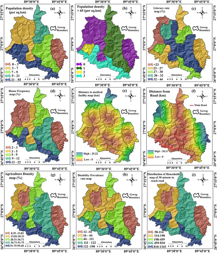
www.nature.com/scientificreports/
responsible for landslides. Among them, landslides caused by road cutting are very common. Landslides are more
likely due to intensive deforestation for farmland. The potential human influence could well be the outcome of
building roadways and other civil constructions on the slopes which are devoid of planning. Blasting is another
addendum to these. The landslide problem is only going to get worse as the world’s population grows, putting
more strain on natural resources. Therefore, the inclusion of these man-made processes as causative factors to
produce a spatial vulnerability map is of utmost importance.
Several studies in the past have considered the role of the geo-environmental factors while few have looked
at the socio-economic aspects of landslide events. Based on the arrangement of anthropogenic and physical
elements in a region, landslides can be accelerated by different geo-environmental as well as socio-economic
factors. With the increasing requirements of the growing population, modification of the land cover for agri-
cultural expansion, road and civil construction, and tourism has influenced the stability of slopes. Therefore, an
effort has been made to analyze the role of both physical and social aspects for spatial vulnerability mapping of
landslides in this s tudy1.
Integration of RS-GIS techniques with knowledge-driven methods or data-mining methods in the landslide
susceptibility as well as vulnerability assessment using spatial and non-spatial data has been widely used11. The
knowledge-driven multi-criteria decision approaches (MCDM) and machine learning models (ML) include
frequency ratio, evidential belief function, logistic regression, weight-of-evidence, fuzzy logic, artificial neural
network, support vector machine, random forest, logistic model tree, boosted regression tree, etc., which are
very widely used in modelling the landslide susceptibility rather than landslide vulnerability11,12. In most cases,
the ML models provided superior results compared to the traditional approaches because the non-linear data
can be adequately treated by the ML models with various scales13. Numerous works have reported that the
ensemble of ML and conventional statistical models provided superior results compared to the single ML model
for modelling landslides14,15.
Along with ML models, recent works have acknowledged deep learning models i.e. convolution neural net-
work (CNN), deep learning neural network (DLNN), recurrent neural network (RNN), etc. as emergent and
more powerful tools for spatial modelling because of better results than the conventional ML models16,17. DLNN
shows many topologies as they appear with more than one hidden layer than that of the single-hidden-layer
neural network. It is used for the extraction, transformation, pattern recognition, and classification tasks of
supervised or unsupervised f eatures17. In the case of CNN model, high detection accuracy for landslide detec-
tion was achieved by Yu et al.18. Ghorbanzadeh et al.19 on the other hand reported contrasting findings of the
CNN approach with three futuristic methods of MLs despite feasibility and high precision. ANN model out-
performed different statistical and ML models in identifying landslide-prone areas as reported by Pourghasemi
and Rahmati20. The deep learning models used in the present study are still not used for vulnerability studies by
the researchers. Previously published landslides susceptibility studies on different parts of Bhutan have revealed
that none of them applied deep learning models to predict susceptibility or vulnerability.
Based on the above-reviewed literature, in the present study, ANN, CNN, and DLNN have been selected
to analyze the landslide vulnerability status of the Chukha district in Bhutan. The risk posed by landslides in
the study region, which is located in the southern part of the country, is mainly due to heavy rainfall during
monsoon21 and weak geology predominantly made of highly fractured and weathered phyllites, slates, and
schists with a high quantity of clay minerals22. The situation is further aggravated due to anthropogenic activities
like road c uttings23. The performance of the above said models were evaluated by the most selective validation
methods and statistical measures. The pixels-based evaluation of landslide models has been done by the relative
landslide density index (R-index) method.
Materials and methods
Study area. The Chukha Dzongkhag (district) lies in the southern foothills of the Bhutan Himalayas (Fig. 1).
It shares border with the neighbouring Indian state of West Bengal and thus serves as a vital route for mutual
trading between the two countries. The major border town of Phuentsholing is the gateway city that connects
India to Western Bhutan. Some of the important hydropower plants such as Chukha and Tala are located in
the Chukha district. Because of proximity to India and ease of accessibility to large Indian market, many of the
country’s industrial infrastructures are located along the foothill flat areas of Chukha district. From the statistic
report of Bhutan Govt., an estimated 4.22% of the entire district (1879.77 km2) comprises of fields cultivated
with oranges and potatoes that constitutes the main source of rural cash income.
In the study area, the monsoon season extends from June–September of each year and about 78% of the
annual rainfall occurs during this period, making the area highly vulnerable to landslide hazards and flooding.
In addition, the rugged mountainous terrain with steep slopes further exacerbates the condition that triggers
the landslides, exposing the area to the vagaries of weather events. The landslides obstruct the national highway
(Phuentsholing-Thimphu Highway) which is the main trade route of the country, causing heavy losses to lives
and infrastructures (Table 1). One of the major landslides in the region was along the Phuentsholing-Thimphu
highway (26.85 N, 89.33 E to 27.15 N, 89.55 E) just after the 2016 monsoon. The intensity and frequency of such
events are expected to increase with climate change, resulting in an increasing risk to the residents and also
affecting the economy of the country.
Methodology. The steps followed in this work are presented in Fig. 2.
(1) Prepared landslide inventory map based on landslide locations identified through field investigation.
(2) Collected data for several geo-environmental and socio-economic factors.
(3) Selected factors using collinearity test and information gain ratio (IGR) methods.
Scientific Reports | (2021) 11:16374 | https://doi.org/10.1038/s41598-021-95978-5 2
Vol:.(1234567890)
www.nature.com/scientificreports/
Figure 1. Location of the study area: (a) Bhutan and (b) Chukha district which is prepared by open source
QGIS 3.16 software (https://qgis.org/en/site/forusers/download.html).
(4) Applied two deep learning approaches i.e. DLNN and CNN, and one benchmark machine learning model
i.e. ANN to produce physical landslide vulnerability, socio-economic landslide vulnerability and overall
landslide vulnerability.
Scientific Reports | (2021) 11:16374 | https://doi.org/10.1038/s41598-021-95978-5 3
Vol.:(0123456789)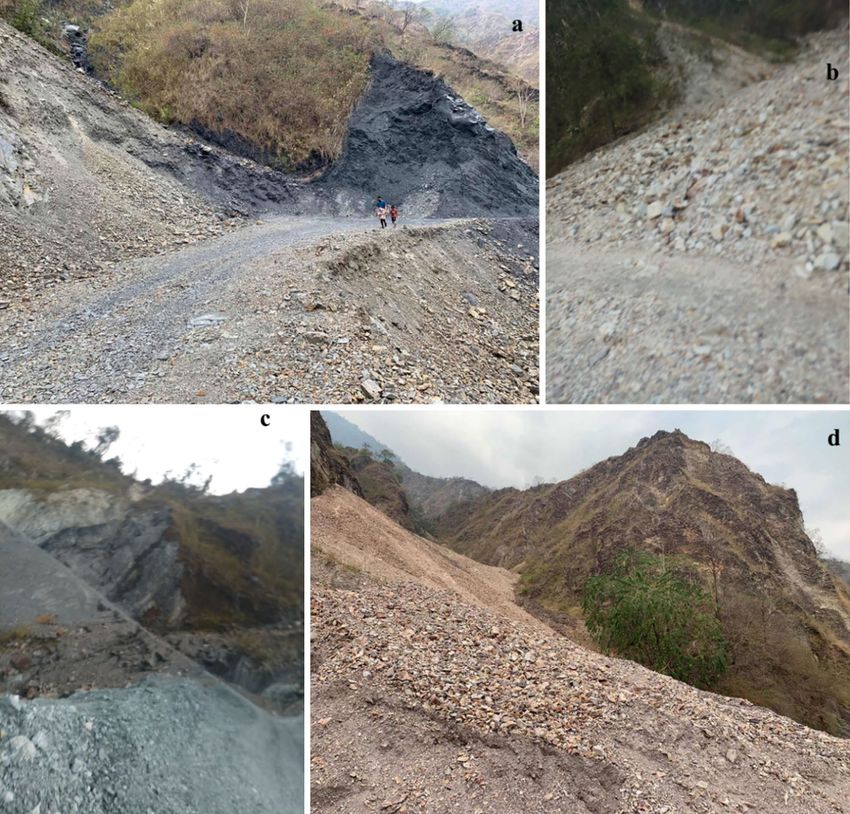
www.nature.com/scientificreports/
Losses caused by the landslides
Name of the area Latitude and longitude Date and time of landslides (properties and lives) Source
Approx
Bhutan Today
Geling gewog (Kamji) 26.90242 N June 16, 2020 Road block
(National news paper, June 17, 2020)
89.51761 E
Approx
(26.89472 N
89.43556 E)—Sorchen Road blocks- nearly 200 vehicles BBS
Sorchen & Kamji July 12, 2019
Approx stranded (National TV, July 12, 2019)
26.90242 N
89.51761 E—Kamji
Approx
Numerous vehicle and houses were Bhutan 24 × 7
Phuentsholing gewog (Kabeytar) 26.86333 N June 25, 2019
damaged (National newspaper, June 26, 2019)
89.39611 E
Approx Killed a 60 year old women and cut off
Kuensel
Phuentsholing gewog (Darjaygang) 26.8775 N August 12, 2017 road connection between Dungna and
(National newspaper, August 13, 2017)
89.38556 E Metedkha gewog
Approx
Massive landslide washed away the sec- Kuensel
Geling gewog (Kamji) 26.90242 N June 23, 2016
tion of road at Kamji (National newspaper, June 24, 2016)
89.51761 E
Table 1. Details of some recent major landslides and losses occurred in the study area.
(5) Analysed significant factors using RF and Chi-square attribute evaluation (CSAE) ML models.
(6) Finally, model performances were analyzed using ROC, AUC, efficiency, accuracy, true positive rate (TRP),
false positive rate (FPR), true negative rate (TNR), false negative rate (FNR), Kappa index, root mean square
error (RMSE), mean absolute error (MAE) and relative landslide density index (R-index) methods.
Preparation of landslide inventory map (LIM). Mapping of the past and present records of landslide
events is called an inventory map24. In this study, these records were collected from the Project Dantak, Border
Road Organisation (BRO), Govt. of India, and from two Royal Government of Bhutan organizations—Depart-
ment of Geology and Mines (DGM) and National Centre for Hydrology and Meteorology (NCHM). For loca-
tion verification, field survey was carried out using Global Positioning System devices in January 2020 (Fig. 3).
A total of 350 landslides were mapped for modelling the relative landslide vulnerability, of which 50.4% are rock
falls, 40.2% are debris slides and 9.4% are rotational slides. Correspondingly, the same amount of non-landslide
points was randomly selected for training and validating the models. Out of the total landslide location, 70% was
used as training dataset and the remaining 30% as testing dataset24.
Preparation of the landslide vulnerability conditioning factors (LVCFs). In this study, 22
geo-environment and 9 socio-economic factors were used for landslide vulnerability modelling which were
obtained from the high-resolution (12.5 × 12.5 m) PALSAR DEM of Alaska DEM facility, Landsat 8OLI/TIRS of
30 m × 30 m resolution from USGS Earth Explorer, the demographic data from the National Statistics Bureau,
Bhutan, rainfall data of last five years from National Centre for Hydrology and Meteorology, and geological map
of 1:500,000 scale from Department of Geology and Mines, Royal Government of Bhutan. The soil resistivity
and textural classes (clay, silt and sand) data were extracted from laboratory tests of collected samples from the
study area. Data processing and modelling were performed using software such as SPSS, MS-Excel, QGIS 3.16,
and R studio.
Geo‑environmental factors. The elevations of the study area vary from a maximum of 4411 m to as low as 98 m
(Fig. 4a) and the slope ranges from 0° to 80° (Fig. 4b). Aspect of slope is classified into nine categories namely,
Flat, North, South, West, East, Northeast, Southeast, Northwest, Southwest (Fig. 4c). The spatial distribution of
plan curvature and profile curvature ranges from − 32.89 to 32.12 (Fig. 4d) and from − 45.17 to 43.52 (Fig. 4e).
The spatial value of convergence index (CI) ranges from − 92.25 to 89.53 (Fig. 4f) and topographical position
index varies between − 17.59 and 26.35 (Fig. 4g). The value of terrain ruggedness ranges from 0 to 40 (Fig. 4h).
The spatial value of topographical wetness index varies between 0.68 and 25.41 (Fig. 4i) and valley depth varies
from 0 to 817 (Fig. 4j). The length of slope and value of relative slope position of this study area ranges between
0 and 119 (Fig. 4k) and from 0 to 1 (Fig. 4l), respectively. Rainfall map was prepared based on the last 5 years’
average annual precipitation data of the different stations using the Inverse Distance Weighted interpolation
method. The average maximum and minimum precipitations for this study area are 4130 mm and 1357 mm,
respectively (Fig. 4n). The land use/land cover (LU/LC) map of the district has been prepared from Landsat 8
OLI/TIRS satellite imagery following the supervised maximum likelihood classification method. The LU/LC
categories are broad leave forest, build-up areas, mixed forest, grassland, miscellaneous, conifer forest, and agri-
culture respectively (Fig. 4p). The normalized differential vegetation index (NDVI) was also generated using
RED and NIR band of Landsat 8OLI/TIRS imagery and values differs from − 0.33 to 0.81 (Fig. 4q). The positive
values of NDVI indicate the dense vegetation cover areas, while the negative values indicate low vegetation cover
areas. The geology of the study can be categorized into Buxa Group, Daling-Shumar Group, the Lesser Himala-
yan zone, Paro formation, and the structurally lower Greater Himalayan zone (Fig. 4r). The soil resistivity values
were determined by surface electrical resistivity method using soil samples and the map depicting resistivity
Scientific Reports | (2021) 11:16374 | https://doi.org/10.1038/s41598-021-95978-5 4
Vol:.(1234567890)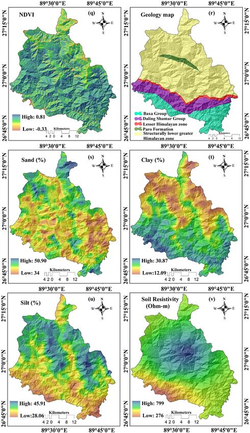
www.nature.com/scientificreports/
Figure 2. Flowchart of the developed methodology.
distribution was prepared applying Inverse Distance Weighted (IDW) interpolation method. The soil resistivity
spatially varies from 276 to 799 Ω-m (Fig. 4v). Following the same method sand, clay, and silt maps were also
prepared. In different parts of the district the percentage of sand, silt, and clay was found to be 34–50%, 12–30%,
and 28–45%, respectively (Fig. 4s, 4t, 4u). Drainage of the study area has been extracted from the open series
topographical maps and DEM. Buffering tool of QGIS 3.16 was used to prepare the distance from the river map
(Fig. 4m) and distance from lineament map (Fig. 4o).
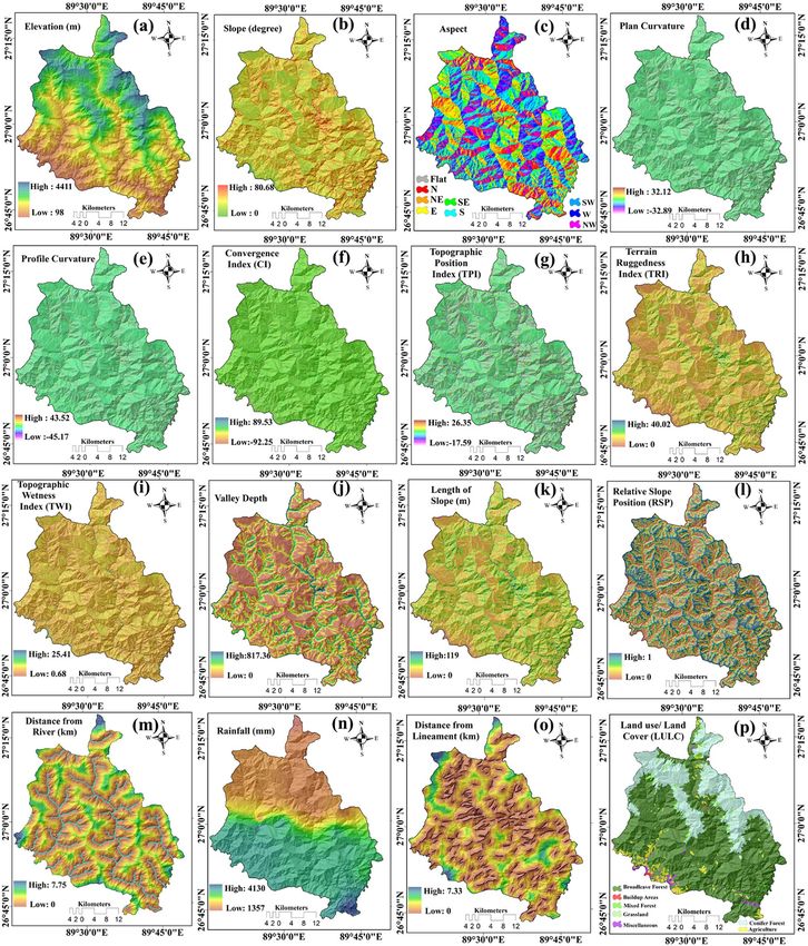
Socio‑economic factors. To identify the social vulnerability of landslides, socio-economic factors were chosen.
The distance from road was prepared using the Euclidian distance buffering tool (Fig. 5f). The demographic
data was derived from the district headquarter of Chukha district, Bhutan. The thematic maps of the population
density, old population density, house frequency, literacy rate, medical facility, disability prevalence rate, number
of households that require at least 30 min to reach the road head (Fig. 5a–i) were prepared in GIS platform based
on the block-wise data.
Scientific Reports | (2021) 11:16374 | https://doi.org/10.1038/s41598-021-95978-5 5
Vol.:(0123456789)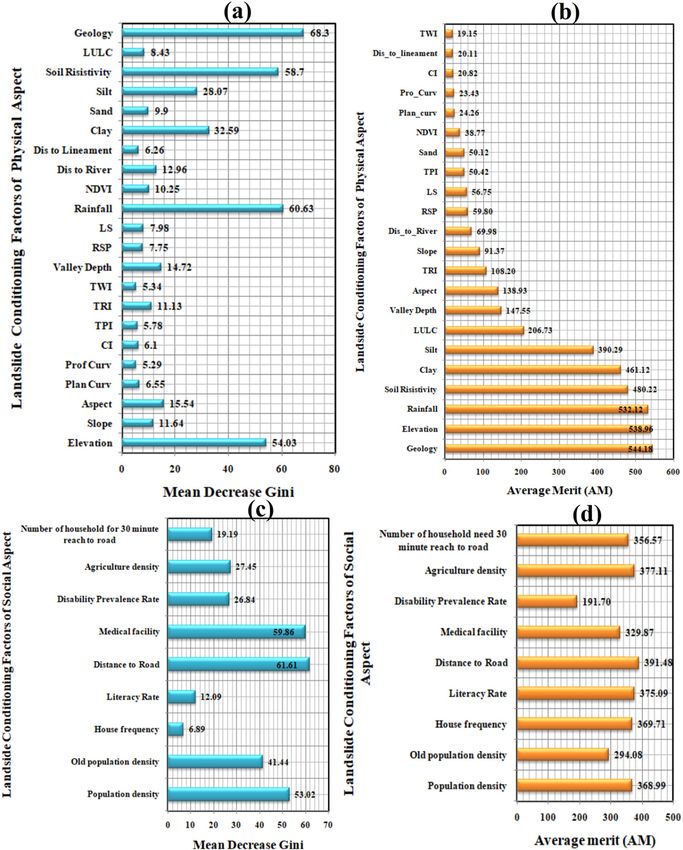
www.nature.com/scientificreports/
Figure 3. Some field photos of landslide events in Sharphug (latitude 26.76 N, longitude 89.7 E), under Darla
Gewog (sub-division) of Chukha Dzongkhag (District).
Factor selection techniques. Collinearity analysis and information gain ratio was used for selecting the
appropriate factors to measure the landslide vulnerability of the Chukha district.
Collinearity analysis (CA). Collinearity is a linear association between two explanatory factors. Two factors are
perfectly collinear if there is an exact linear relationship between them which can influence the model result. The
collinearity test was performed using the Variance Inflation Factor (VIF) and Tolerance (TOI)25. A tolerance of
less than 0.2 and a VIF of > 5 indicates a multicollinearity problem26. Based on the diagnosis, a total of 22 geo-
environment and 9 socio-economic factors have been selected to proceed with the modelling.
Information gain ratio (IGR) method. The information gain ratio (IGR) is one of the machine learning
techniques27 which evaluates the correlations of landslide occurrence with landslide conditioning factors and the
role of these factors in the frequency of their correlations28. The IGR is employed to reduce a bias to multi-value
property, taking into account the size and number of sections, when selecting a function. The IGR for element
TWI, for example, is estimated as:
Scientific Reports | (2021) 11:16374 | https://doi.org/10.1038/s41598-021-95978-5 6
Vol:.(1234567890)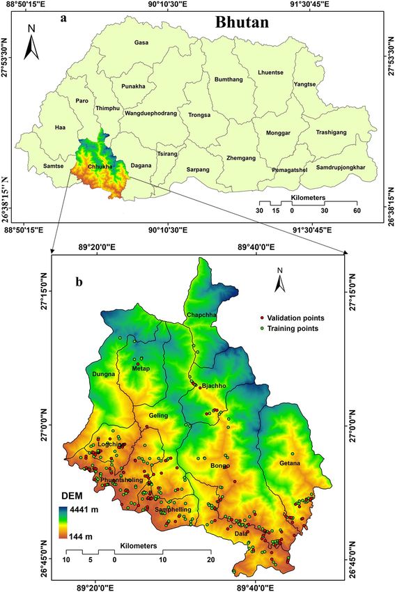
www.nature.com/scientificreports/

                                  Figure 4.  Factors used for producing the landslide susceptibility maps—(a) Elevation, (b) Slope, (c) Aspect,
                                  (d) Plan curvature, (e) Profile curvature, (f) Convergence index, (g) Topographical position index, (h) Terrain
                                  ruggedness index, (i) Topographical wetness index, (j) Valley depth, (k) Length of slope, (l) Relative slope
                                  position, (m) Distance from river, (n) Rainfall, (o) Distance from lineament, (p) Land use/land cover, (q)
                                  Normalized differential vegetation index (NDVI), (s) Geology map, (s) Sand, (t) Clay, (u) Silt, (v) Soil resistivity.

                                                                                         Info(S) − Info(S, TWI)
                                                                       IGR(S, TWI) =                                                                (1)
                                                                                            SplitInfo(S, TWI)

Scientific Reports |   (2021) 11:16374 |               https://doi.org/10.1038/s41598-021-95978-5                                                     7

                                                                                                                                                Vol.:(0123456789)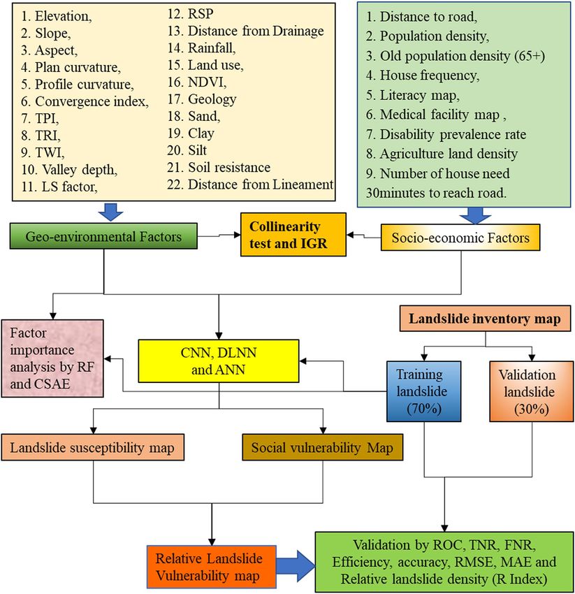
www.nature.com/scientificreports/
Figure 4. (continued)
m
Sj
Sj
SplitInfo(S, TWI) = − log2 (2)
j=1 |S| |S|
where SplitInfo and S are represented potential information conducted by partitioning S into m subset and
training28.
Scientific Reports | (2021) 11:16374 | https://doi.org/10.1038/s41598-021-95978-5 8
Vol:.(1234567890)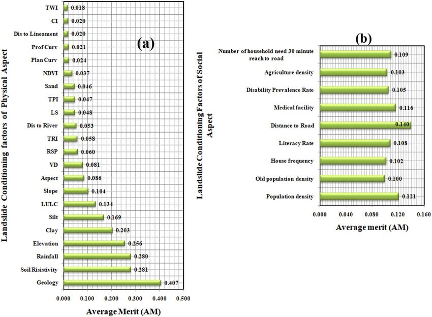
www.nature.com/scientificreports/

                                  Figure 5.  LVCFs used for producing the socio-economic landslide vulnerability maps: (a) Population density,
                                  (b) Old population density, (c) Literacy rate, (d) House frequency, (e) Distance to medical facility, (f) Distance
                                  to road, (g) Agriculture density, (h) Disability prevalence rate, (i) Household need 30 min to reach road.

Scientific Reports |   (2021) 11:16374 |               https://doi.org/10.1038/s41598-021-95978-5                                                      9

                                                                                                                                               Vol.:(0123456789)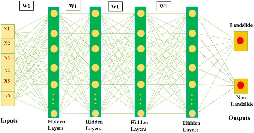
www.nature.com/scientificreports/
Figure 6. Theoretical structure of used CNN model.
Applied deep learning and benchmark machine learning approaches
Artificial neural network (ANN). One of the most popular ANN used for landslide susceptibility is the
Multi-layer perceptron Neural Network (MLP-NN)29. Basically, three layers which include an input layer, one
hidden layer, and an output layer were involved in the topology of MLP-NN m odels30. Although their output is
regulated by their structure, the activation functions and the updating of the link weights between the process-
ing components31. The MLP-NN was introduced in the current study based on the "RSNNS" R package32 and by
using a grid search technique, the number of the hidden processing elements was tuned.
Convolution neural network (CNN). DLAs are modelled on the structure of the human brain and based
on an ANN. CNN, introduced by LeCun et al.33 is a well-known deep learning algorithms (DLA). Recently,
a number of disciplines, including earth science, have been increasingly using CNN for classification and
prediction34. The utilisation of several layers, pooling, local connections, and mutual weighting distinguishes
CNN from traditional neural networks. The central concept behind CNN is that images are used as input param-
eters. The set of indicators can be greatly decreased and processing can be accelerated. The convolution layers
(CLs), pooling layers (PLs), and linear rectified unit layers are involved in the typical structure of CNN model
(Fig. 6). CLs deliver the best data classification results by learning the convolutions. By decreasing the quantity of
convolution architectures, PLs control overfitting that allows consistent conversion and enhances computational
efficiency35. The ReLU improves the network’s nonlinear capabilities by ReLU activation. Researchers have cre-
ated and applied numerous analysis structures based on data form, image, and purpose, including G oogleNet36,
ZFNet37, and VGGNet38 among the more common structures. Several articles have clarified these layer forms,
their basic learning criteria, and how the CNN processes the data for training33. The CNN-2D structure is used
here because it is relevant for earth science s tudies39. The input data in CNN must be 1-D images: a 1-D input
grid cell (vector) with different features which be translated into a 2-D input grid cell to ensure optimum initiali-
zation efficiency and this technique is used for mapping landslide vulnerability. In current research, we compare
the number of LCVFs to the number of attribute values for each factor, and the larger of the two numbers is used
to determine the size of the related two-dimensional matrix. The research region, for example, contains 25 geo-
logical categories, which is more than the number of LCVFs. As a result, for each grid cell, we created a 25 × 25
matrix. Since there is no sorting of data and analysis is continuous, the images are large.
Scientific Reports | (2021) 11:16374 | https://doi.org/10.1038/s41598-021-95978-5 10
Vol:.(1234567890)www.nature.com/scientificreports/
Figure 7. Configuration of the DLNN approach.
Deep learning neural networks (DLNN). The major advantage of DLNN model is that it uses raw data-
set to create a high-level function18. DLNN comprises of three layers—an input layer, followed by hidden layers
which lead to output layers40. Figure 7 demonstrates the conceptual setup of the DLNN model included in this
analysis. The overall pattern of DLNN model is to work in such a way that the input layer delivers the signals that
are diverse landslide factors, and after processing and interpretation of this information in multiple hidden lay-
ers, the impacts are shown in the model’s last year, the output layer. The output layer has two probable labels, i.e.
a negative label (non-landslides) and a positive label (landslides). From the last hidden layer, these classification
results are collected and displayed in the output layer41. DLNN has unique advantages over the conventional ML
algorithm, and therefore much more attention has been put on the use of the DLNN model in the area of predic-
tion analysis. DLNN outperforms all other ML models in several ways, by making optimum use of unstructured
data by specific observations to recognize the training dataset, being versatile enough as to identify new data,
and being able to create new learning models by introducing more layers to the neural network architecture.
Mathematical equation mentioned below was applied in DLNN as per the Kim40:
x if x > 0 x if x > 0
h(x) =
0 if x < 0
= max(0, x) h(x) =
0 if x ≤ 0
= max(0, x) (3)
where x is an input signal, and h is an activation function. The following can be represented on the basis of the
ReLU activation function as:
1 if x > 0
h(x) =
0 if x ≤ 0 (4)
The cost function is the distinction between class outcomes that are experiential and expected. The loss func-
tion (L) of a cross-entropy is used to detect patterns and is given by:
ND
L = − N1D T1n(Y ) + (1 − T)1n(1 − Y ) (5)
n=1
where, the number of the training data sets is expressed by ND , T indicates the class outputs detected and Y
displays the class outputs expected.
Methods used for validating the models
Receiver operating characteristics (ROC) curve. For any two distinct vectors where the first vector
describes the binary presence-absence state of a particular action and the second vector gives the related prob-
ability predictions, the ROC curve can be prepared which is a common cut-off dependent d iagnosis42,43. The
overall model success can be recognized based on AUC values, as per the classification provided by Hosmer and
Lemeshow44. There are four major elements of ROC curve: e true positive (P), false positive (Q), false negative
(R) and true negative. The following measures including sensitivity or true positive rate (TPR), false positive rate
(FPR), true negative rate or specificity (TNR), false negative rate or miss rate (FNR), efficiency, precision, nega-
tive predictive value (NPV), Matthews correlation coefficient (MCC) and Cohen’s Kappa have been computed
from these elements for validating the models:
P P
TPR = = (6)
X P+R
Scientific Reports | (2021) 11:16374 | https://doi.org/10.1038/s41598-021-95978-5 11
Vol.:(0123456789)www.nature.com/scientificreports/
Q Q S
FPR = = =1− (7)
Y Q+S S+Q
S S
TNR = = (8)
Y S+Q
Q Q
FNR = = = 1 − TPR (9)
X Q+P
P+S
Efficiency accuracy = (10)
T
where X, Y and T are the number of landslides, non-landslides and sum of total landslides and non-landslides,
respectively
P
Precision = (11)
P+Q
S
NPV = (12)
S+R
(P × S) − (Q × R)
MCC = √ (13)
(P + Q)(P + R)(S + Q)(S + R)
(P + S) − [(P + R)(P + Q) + (R + S)(Q + S)]/T
Cohen’s Kappa = (14)
T − [(P × S))(P + Q) + (R + S)(Q + S]/T
RMSE. The root mean square error (RMSE) was determined on the basis of the variations between the values
expected by a model and the values actually observed (Eq. 9):
2
N P
i=1 − P (15)
RMSE =
N
and P is predicted and observed values of dependent variable, respectively.
where N is sample size, P
MAE. Mean absolute error (MAE) is measured as the sum of the differences between the expected value and
the actual value of the model, without taking their direction into account:
1
n
MAE =
P − P
(16)
N
i=1
and P are predicted and observed values of dependent variable, respectively.
where N is sample size, P
Relative landslide density (R‑Index). R-index was used to evaluate the vulnerability maps of landslides.
R-index is calculated as following45.
R = ((xi/Xi)/ (xi/Xi)) × 100 (17)
where xi is the percentage of the area that is vulnerable to landslides in each vulnerability class, and Xi is the
percentage of landslides in each vulnerability class. The maximum values of these vulnerability classes indicate
the highest goodness-of-fit and excellent a ccuracy46.
Results
Multicollinearity assessment. The findings of collinearity results indicate that no linearity exists among
the LVCFs because the Tolerance and VIF values of these factors do not surpass their limits (Table 2) which sug-
gests the aptness for inclusion in the modelling.
Results of IGR. The result of IGR method is shown in Fig. 8. The IGR values of the geo-environmental
LVCFs for landslide vulnerability prediction were higher for geology, soil resistivity, rainfall, and elevation
(Fig. 8a) and for socio-economic LVCFs, it is higher for distance to road and population density (Fig. 8b).
Landslide vulnerability analysis. Using the three models i.e. ANN, CNN, and DLNN and consider-
ing three aspects of vulnerability i.e. geo-environmental, socio-economic, and relative or overall vulnerability,
Scientific Reports | (2021) 11:16374 | https://doi.org/10.1038/s41598-021-95978-5 12
Vol:.(1234567890)www.nature.com/scientificreports/
Collinearity statistics
LVCFs Tolerance VIF
Geo-environment factors
Elevation 0.272 3.812
Slope 0.348 2.706
Aspect 0.898 1.113
Plan curvature 0.390 2.562
Profile curvature 0.282 3.547
Convergence index 0.517 1.933
Topographic position index 0.146 6.844
Terrain ruggedness index 0.270 4.286
Topographic wetness index 0.351 2.848
Valley depth 0.323 3.100
Relative slope position 0.327 3.059
Length of slope 0.181 5.521
Rainfall 0.269 3.723
NDVI 0.778 1.285
Distance from river 0.605 1.653
Socio-economic factors
Population density 0.665 1.323
Old population density 0.273 3.646
House frequency 0.263 3.808
Literacy rate 0.233 4.286
Distance from road 0.266 3.765
Medical facility 0.627 1.596
Disability prevalence rate 0.123 8.114
Agriculture density 0.232 3.556
Number of the household for 30 min to reach road 0.334 2.269
Table 2. Collinearity results of LVCFs.
a total of 9 landslide vulnerability maps were derived which are ANN-LS (landslide susceptibility), ANN-SV
(social vulnerability), ANN-RLV (relative landslide vulnerability), CNN-LS, CNN-SV, CNN-RLV, DLNN-LS,
DLNN-SV, DLNN-RLV. Accepting natural breaks classification method, these landslide susceptibility maps were
classified into five vulnerability zones: very low, low, moderate, high, and very high. The ANN-LS, CNN-LS, and
DLNN-LS maps have 16.57%, 18.74%, and 17.75% area of the district as very high vulnerable for landslides from
the scenario of geo-environmental setup. Similarly, ANN-SV, CNN-SV, and DLNN-SV maps have provided the
socio-economic status of vulnerability as very high of 14.49%, 14.55%, and 14.40% area, respectively. In case of
relative vulnerability maps ANN-RLV, CNN-RLV and DLNN-RLV have quantified 15.46%, 18.80%, and 14.66%
of area as most vulnerable to landslides. The very high vulnerable zones have mostly occurred in the southern,
south-west and south-east portion of the district and very low vulnerability is found in northern, north-east, and
north-west regions. These results appear to be associated with the presence of weak geology, heavy rainfall dur-
ing monsoon, and Phuentsholing-Thimphu national highway that passes through the first three portions of the
district. Apart from this, rapid population growth in the above areas due to the fast development of Phuentshol-
ing, the business city of Bhutan, resulted in new anthropogenic activities and thus weakening the soil (Fig. 9).
The spatial extension of other vulnerability classes is given in Fig. 10.
Validation. Table 3 shows the comprehensive results of the ROC curve and other validation measures. The
AUC computed using train data indicates success rate and AUC computed using test or validation data denotes
prediction rate of the models47. Using the training data, AUC of ANN-LS, ANN-SV and ANN-RLV models are
0.893, 0.864, and 0.907 and using validation dataset these are 0.887, 0.846 and 0.902 respectively. The AUC using
train and validation data are 0.912, 0.910 in CNN-LS; 0.893, 0.872 in CNN-SV and 0.921 and 0.928 in CNN-
RLV models respectively. The AUC values of DLNN model are 0.880 (DLNN-LS), 0.867 (DLNN-SV) and 0.901
(DLNN-RLV) in the training case and 0.890 (DLNN-LS), 0.852 (DLNN-SV) and 0.900 (DLNN-RLV) in the vali-
dation case. Among these models, the CNN-RLV model has achieved the highest performance in terms of the
AUC, accuracy, efficiency, kappa and predictive values and all other measures (Table 3). The result of reliability
measures such as MAE and RMSE value is lowest for CNN-RLV followed by DLNN-RLV and ANN-RLV model.
The R-index values for each model using geo-environmental aspect, socio-economic aspect or overall factors, is
highest for very high vulnerability class followed by high vulnerability class (Table 4; Fig. 11).
Scientific Reports | (2021) 11:16374 | https://doi.org/10.1038/s41598-021-95978-5 13
Vol.:(0123456789)www.nature.com/scientificreports/
Figure 8. Average merit of LVCFs: (a) geo-environment factors, (b) socio-economic factors.
Factors importance analysis. The importance of the LVCFs in predicting landslide vulnerability was
evaluated by random forest (RF) and chi-square attribute evolution technique (CSAE). The outcome of RF
showed that the geology, rainfall, soil resistivity, and elevation were the most predictive factors for landslide
vulnerability modelling in this research, followed by the sand and silt distribution and other geo-environment
LVCFs (Fig. 12a). Among the socio-economic LVCFs, distance to road, population density factors have the most
importance (Fig. 12c). The CSAE method yielded similar results to the RF model (Fig. 12b,d).
Discussions
Identifying or mapping the areas with future landslide potential is one of the most useful document for appro-
priate land use planning and mitigation decision m aking13,47,48. Evaluation of landslide susceptibility and vul-
nerability of a hilly area (as mountainous areas are subjected to the landslides) is indeed, necessary as it will
serve as an essential dataset which will be used for identifying the points and places of relatively high landslide
susceptibility and vulnerability which can be utilized for efficient and safe planning, design as well as the con-
struction activities in an identified landslide zone. In the studied region, as well as other similar locations, there
has been a significant growth in human socio-economic activities as well as other geo-environmental variables
in recent decades. As a result, the frequency with which landslides occur in certain locations has risen. Such
occurrences result in a significant loss of human life and property, as well as it results in a negative impact on
different sectors such as tourism and infrastructure development49. A better working LVM has always been a
subject of significant relevance within the community of numerous scholars across the world who are research-
ing and investigating landslides. This is due to the fact that the methodology and conditioning factors used can
have a substantial impact on the models’ predictive performance48. It is very relevant to employ the mechanisms
of factor selection to maximize the efficiency of landslide models by eliminating unwanted or trivial variables
before training t hose50. CA and IGR method was adopted to accomplish this. In this study, CA revealed that all
of the conditioning variables were effective and independent. In order to pick the most appropriate conditioning
factor, there must be a non-collinear link between the LVCFs, which may be done via multicollinearity analysis51.
Applying CA and IGR analysis, this study took into account a total of twenty-two geo-environmental and nine
socio-economic factors, and the incorporation of these LVCFs has been justified in several s tudies4,5,21. It is very
important to select LVCFs associated with past and present landslide events in vulnerability modelling. Although
Scientific Reports | (2021) 11:16374 | https://doi.org/10.1038/s41598-021-95978-5 14
Vol:.(1234567890)www.nature.com/scientificreports/
Figure 9. Physical, social and relative landslide vulnerability maps produced by: (a) ANN-LS, (b) ANN-SV, (c)
ANN-RLV, (d) CNN-LS, (e) CNN-SV, (f) CNN-RLV, (g) DLNN-LS, (h) DLNN-SV and (i). DLNN-RLV.
landslides are quasi-natural hazard but when it results in destruction and harm to the economy and society, it
indicates the association of socio-economic causes in the event happened. Therefore, to enhance the performance
of modelling, this research was conducted taking into consideration both physical and social aspects; these fac-
tors are found to be very significant, especially in hillslope r egions52.
The study was approached towards mapping the landslide vulnerability considering geo-environmental and
socio-economic aspects to improve the classification accuracy using deep learning and benchmark machine
learning methods viz. CNN, DLNN and ANN. In all cases of vulnerability mapping (Physical, socio-economic
Scientific Reports | (2021) 11:16374 | https://doi.org/10.1038/s41598-021-95978-5 15
Vol.:(0123456789)www.nature.com/scientificreports/
Figure 10. Distribution of physical, social and relative vulnerability classes produced using three models.
and combined) opted in this study, CNN has shown the best result followed by DLNN and ANN. In terms of
the validation measures, the CNN-RLV model had the highest goodness-off-fit and excellent predictive perfor-
mance, followed by the CNN-LS, CNN-SV, DLNN-LS, DLNN-S, DLNN- RLV, ANN-LS, ANN-SV and ANN-
RLV models. Sadighi et al.53 for landslide susceptibility assessment used MLP-NN with a Back-Propagation
algorithm (BPANN), Adaptive Neuro-Fuzzy Inference System (ANFIS) models. However, result of models shows
that the ANFIS-ICA had the superior results but ANN had quite good predictive accuracy i.e. AUC of 88.8%.
In this study, ANN-RLV model has assured 88.7% success rate by the application of the AUC measure which
is similar to the aforementioned study. In landslide susceptibility assessments, Bui et al.9 used a DLNN model
and compared its predictive efficiency with state-of-the-art machine learning models in Kon Tum province,
Vietnam. Using ROC curve, the performance of the models revealed that the DLNN model had the highest
goodness-of-fit and outperforming ANN, SVM model. Relatively better performance of DLNN than of ANN was
also achieved in landslide vulnerability mapping for the present research. The efficiency of deep learning models
compared to ML models was found to be better as per the study of Yao et al.54 where authors have developed
the deep neural network model based on semi-supervised analysis (SSL-DNN) for the landslide susceptibility
estimation. For comparison, supervised models were introduced, including deep neural network (DNN), SVM,
and logistic regression (LR). The result revealed that all comparable models were surpassed by the proposed
SSL-DNN (AUC = 0.898) which is greatly supportive of outcome of the deliberating research. Application and
enhanced competence of DLNN model can also be found in other hazard vulnerability and susceptibility map-
ping as Band et al.55 proposed a DLNN model and an ensemble particle swarm optimization (PSO) algorithm
with DLNN (PSO-DLNN), for gully erosion susceptibility mapping. These models were compared with ANN
and SVM model. The PSO-DLNN model has the highest efficiency followed by the ANN and SVM. Therefore,
the derived outcome of this research has a similar covenant to the very previous studies delegating relevance
of adopted methodological scheme. Above all, r, the convolution neural network (CNN) model has provided
superior results outperforming DLNN and ANN models in all of the social vulnerability, landslide susceptibility
and relative or combined vulnerability assessment as exposed by all the adopted validation measures both in
training set and testing set based analysis (Table 4). Therefore, accuracy of the DLNN model was better than the
Scientific Reports | (2021) 11:16374 | https://doi.org/10.1038/s41598-021-95978-5 16
Vol:.(1234567890)www.nature.com/scientificreports/
Matrices ANN-PV ANN-SV ANN-RLV CNN-PV CNN-SV CNN-RLV DLNN-PV DLNN-SV DLNN-RLV
Training dataset
TPR 0.81 0.77 0.82 0.84 0.80 0.86 0.83 0.79 0.83
FPR 0.16 0.20 0.14 0.13 0.17 0.10 0.15 0.18 0.13
TNR 0.84 0.80 0.86 0.87 0.83 0.90 0.85 0.82 0.87
FNR 0.19 0.23 0.18 0.16 0.20 0.14 0.17 0.21 0.17
Accuracy 0.82 0.78 0.84 0.85 0.81 0.88 0.84 0.80 0.85
PPV 0.85 0.80 0.86 0.88 0.83 0.90 0.85 0.83 0.87
NPV 0.79 0.76 0.81 0.83 0.79 0.85 0.81 0.77 0.82
MCC 0.65 0.57 0.68 0.70 0.63 0.76 0.69 0.61 0.70
Cohen’s Kappa 0.65 0.57 0.68 0.70 0.63 0.75 0.69 0.61 0.70
AUC 0.866 0.858 0.887 0.912 0.893 0.921 0.898 0.887 0.911
MAE 0.150 0.187 0.101 0.032 0.064 0.013 0.040 0.089 0.028
RMSE 0.387 0.432 0.318 0.180 0.254 0.114 0.199 0.299 0.169
Validation dataset
TPR 0.82 0.82 0.86 0.89 0.86 0.92 0.88 0.85 0.90
FPR 0.11 0.17 0.10 0.09 0.12 0.07 0.09 0.15 0.09
TNR 0.89 0.83 0.90 0.91 0.88 0.93 0.91 0.85 0.91
FNR 0.18 0.18 0.14 0.11 0.14 0.08 0.12 0.15 0.10
Accuracy 0.85 0.83 0.88 0.90 0.87 0.92 0.90 0.85 0.90
PPV 0.90 0.83 0.90 0.92 0.89 0.93 0.92 0.85 0.90
NPV 0.81 0.82 0.85 0.89 0.86 0.92 0.88 0.85 0.91
MCC 0.71 0.65 0.75 0.81 0.74 0.85 0.79 0.71 0.81
Cohen’s Kappa 0.71 0.65 0.75 0.81 0.74 0.85 0.79 0.71 0.81
AUC 0.857 0.846 0.879 0.910 0.872 0.928 0.890 0.852 0.900
MAE 0.069 0.103 0.044 0.023 0.027 0.011 0.024 0.067 0.022
RMSE 0.263 0.321 0.209 0.153 0.163 0.104 0.155 0.259 0.150
Table 3. Results of validation measures based on training and validation datasets.
conventional ANN machine learning technique. This is because greater number of samples and huge data could
be handled by this model and the outcomes can be estimated with greater precision. The key benefit of deep
learning is its formal system of self-governing DLNN layer organization learning. The conventional machine
learning is incapable of processing such a vast number of inputs, and the result is less optimal in comparison to
the deep learning m odel55. The accuracy of machine learning for different purposes was substantially enhanced
in deep learning systems55. Yi et al.50 developed a convolutional neural network (CNN) model for the spatial
prediction of landslides. The result of CNN was compared with three conventional ML algorithms, i.e., logistic
regression, multilayer perceptron (MLP) neural network and radial basis function (RBF) neural network which
found CNN as the best fitted and excellent predictive model, followed by the MLP, logistic regression RBF. Wang
et al.39 applied the deep learning and ML models such as logistic regression, SVM, RF models for LS assessment.
The result of that research also proved that CNN had the highest performance of predictive modelling followed
by the ML models. With the agreement of the results of these studies, the present work also confirms the rela-
tively highest adaptability of CNN model in deriving LVMs as reflected in the produced results of validation and
accuracy measures. ReLU activation function was applied in the present study considering the aforesaid litera-
ture. The advantages of CNN model are that it considers all the neighbourhood information and can determine
manifold stages of representations from input data56. It maintains the association of pixels using several factors
and identifying internal e lements59.
Following Jenk’s algorithm of natural breaks classification, LVMs were divided into five groups of susceptibility
classes. This strategy of clustering data helps to reduce the mean–variance of each class from the mean within
class range and to increase the discrepancy between each class from the means of the other c lasses57. From the
analysis of the LVMs of this study, the very high vulnerability zone of landslide is found in the southern, south-
western and south-eastern portion where the soil resistivity and geology is very weak. The amount of annual
average precipitation is maximum in this part of the district. With very high elevation and steep slope, certain
geological configurations influenced by socio-economic aspects tend to become unstable causing landslide.
Phuentsholing is a highly urbanized centre located in the south upland slope with dense road network built
through modification of the general slope that accelerates landslide processes.
Landslides are caused by a number of factors in a given area, but not all of them are equally responsible.
During the field investigation, it was found that the landslides in the study region are caused by both natural
causes (geological structure, heavy rainfall and very steep slope) as well as by human interferences (such as
slope cutting for the construction of road, deforestation for expansion of agricultural land) which makes the
area vulnerable to landslide. Relative landslide density index (R), in this work, helped to analyse the association
Scientific Reports | (2021) 11:16374 | https://doi.org/10.1038/s41598-021-95978-5 17
Vol.:(0123456789)www.nature.com/scientificreports/
Models Classes No. of pixels % of pixels No. of landslides % of landslides R-index
Very low 5,607,364 46.58 21 6.11 2
Low 1,547,452 12.85 45 12.86 15
ANN-P Moderate 1,598,676 13.28 47 13.50 16
High 1,291,334 10.73 29 8.36 12
Very high 1,994,494 16.57 207 59.16 55
Very low 5,573,335 46.29 38 10.93 3
Low 1,739,451 14.45 21 6.11 6
ANN-S Moderate 1,546,377 12.84 82 23.47 27
High 1,435,333 11.92 51 14.47 18
Very high 1,744,824 14.49 158 45.02 46
Very low 5,269,576 43.77 1 0.32 0
Low 2,369,894 19.68 6 1.61 1
ANN-RLV Moderate 1,121,903 9.32 33 9.32 14
High 1,416,707 11.77 93 26.69 31
Very high 1,861,241 15.46 217 62.06 54
Very low 6,013,570 49.95 1 0.32 0
Low 1,438,915 11.95 8 2.25 3
CNN-P Moderate 1,207,156 10.03 20 5.79 9
High 1,123,336 9.33 60 17.04 28
Very High 2,256,343 18.74 261 74.60 61
Very low 4,891,668 40.63 2 0.64 0
Low 1,678,914 13.95 7 1.93 2
CNN-S Moderate 1,453,602 12.07 32 9.00 11
High 2,263,865 18.80 96 27.33 22
Very high 1,751,272 14.55 214 61.09 64
Very low 5,376,679 44.66 1 0.32 0
Low 1,714,734 14.24 5 1.29 1
CNN-RLV Moderate 1,339,692 11.13 20 5.79 8
High 1,344,707 11.17 61 17.36 25
Very high 2,263,507 18.80 263 75.24 65
Very low 5,609,514 46.59 8 2.25 1
Low 1,634,496 13.58 10 2.89 3
DLNN-P Moderate 1,258,738 10.46 27 7.72 12
High 1,399,513 11.62 55 15.76 21
Very high 2,137,060 17.75 250 71.38 63
Very low 5,173,934 42.98 5 1.29 0
Low 1,651,690 13.72 8 2.25 2
DLNN-S Moderate 1,929,658 16.03 32 9.00 8
High 1,549,959 12.87 98 27.97 31
Very high 1,734,078 14.40 208 59.49 59
Very low 5,286,053 43.91 5 1.29 0
Low 2,235,567 18.57 9 2.57 2
DLNN-RLV Moderate 1,304,946 10.84 25 7.07 9
High 1,448,229 12.03 102 29.26 33
Very high 1,764,525 14.66 209 59.81 56
Table 4. Relative landslide density index of susceptibility classes of LSM models.
between produced vulnerability classes of landslide models and percentage of inventory landslides. The highest
R-index value can be found in very high vulnerability class of each model followed by high vulnerability class
which is positive for validating models.
The factor importance using RF (mean decrease Gini) and CSAE (average merit) represented the most
important predictive LVCFs which are fittingly prominent in the southern part of the district (Fig. 12). Among
the physical conditioning factors, both the RF and CSAE based evaluation has identified elevation, rainfall, geol-
ogy, soil resistivity, soil clay and silt percentage etc. as the foremost persuasive factors for land sliding. The alike
importance of the factors has reflected in several pieces of research such as elevation has been identified as a criti-
cal LVCF in various literature since most landslides occur in mountainous regions with a specific gradient4,7,10.
Landslides are influenced by the structure, ordination, age, and exposure of the underlying s urface52. The soil
Scientific Reports | (2021) 11:16374 | https://doi.org/10.1038/s41598-021-95978-5 18
Vol:.(1234567890)www.nature.com/scientificreports/
Figure 11. ROC curves used for validation of landslide vulnerability models: (a) ANN-LS, ANN-SV and
ANN-RLV using Training, (b) ANN-LS, ANN-SV and ANN-RLV using validation datasets, (c) CNN-LS,
CNN-SV and CNN-RLV using Training, (d) CNN-LS, CNN-SV and CNN-RLV using validation, (e) DLNN-LS,
DLNN-SV and DLNN-RLV using training, (f) DLNN-LS, DLNN-SV and DLNN-RLV using validation datasets.
resistivity parameter has a positive connection with landslide susceptibility, showing that reducing soil resistance
upturns the chance of a landslide, especially at higher elevations. Increased soil clay and silt content at medium
to high altitude and upslope areas remain more unstable due to lower integrity than rocky sections, making it
more vulnerable to seepage erosion, liquefaction, and fluidization. However, the type of soil and the amount of
vegetation cover plays an important influence in this46. Among the socio-economic factors, RF and CSAE method
have recognised distance to road, population density, agricultural density, house frequency factor as crucial
Scientific Reports | (2021) 11:16374 | https://doi.org/10.1038/s41598-021-95978-5 19
Vol.:(0123456789)www.nature.com/scientificreports/
Figure 12. Importance of the LVCFs: (a) mean decrease Gini of geo-environmental LVCFs by RF, (b) average
merit of geo-environmental LVCFs by CSAE, (c) mean decrease Gini of socio-economic LVCFs by RF, (d)
average merit of socio-economic LVCFs by CSAE.
Scientific Reports | (2021) 11:16374 | https://doi.org/10.1038/s41598-021-95978-5 20
Vol:.(1234567890)www.nature.com/scientificreports/
for making the area landslide vulnerable. A negative correlation exists for the distance to road LVF, indicating
that the severity of possible landslide events increases in places as roads get closer, and vice versa. A substantial
amount of work by Chan et al.58, Weigand et al.59 has established the role of these factors in triggering landslides.
Conclusion
Landslides have been seen in recent decades as the most critical natural risk that poses serious threat to both
life and property all over the world. Thus short-term and long-term solutions are considered necessary to con-
front these daunting challenges. The landslide vulnerability map has recently become an important means of
delineating landslide-prone regions and management. With the aid of sophisticated methods, proper data, and
integration of remote sensing and a geographical information system, this can be accomplished. DLNN, ANN,
and convolution neural network (CNN) models were used and r all aspects of a landslide event were considered
which are novel approaches to perform the landslide vulnerability mapping of the district. Therefore, along with
geo-environmental data, potential socio-economic factors were also considered as LVCFs using advanced factor
selection techniques. CNN model achieved highest accuracy in modelling the vulnerability in the study area. As
per the finding of the models, lower part of the district is highly susceptible and it needs immediate measures for
managing. For the landslide risk supervision in the present and also for the future, the LVM can suggest imple-
menting different management strategies like afforestation, barrier construction, and proper land use planning.
Received: 8 February 2021; Accepted: 3 August 2021
References
1. Thongley, T. & Vansarochana, C. Landslide susceptibility assessment using frequency ratio model at Ossey watershed area in
Bhutan. Eng. Appl. Sci. Res. 48(1), 56–64 (2021).
2. Kashyap, R., Pandey, A. C. & Parida, B. R. Spatio-temporal variability of monsoon precipitation and their effect on precipitation
triggered landslides in relation to relief in Himalayas. Spat. Inf. Res. https://doi.org/10.1007/s41324-021-00392-8 (2021).
3. Nor Diana, M. I., Muhamad, N., Taha, M. R., Osman, A. & Alam, M. Social vulnerability assessment for landslide hazards in
Malaysia: A systematic review study. Land 10(3), 315 (2021).
4. Ram, P. & Gupta, V. Landslide hazard, vulnerability, and risk assessment (HVRA), Mussoorie township, Lesser Himalaya, India.
Environ. Dev. Sustain. https://doi.org/10.1007/s10668-021-01449-2 (2021).
5. Kumar, P., Mital, A., Ray, P. C. & Chattoraj, S. L. Landslide hazard and risk assessment along nh-108 in parts of Lesser Himalaya,
Uttarkashi, using weighted overlay method. In Geohazards (eds Gali, M. L. & Raghuveer-Rao, P.) 163–180 (Springer, 2021).
6. Li, Y., Chen, L., Yin, K., Zhang, Y. & Gui, L. Quantitative risk analysis of the hazard chain triggered by a landslide and the generated
tsunami in the Three Gorges Reservoir area. Landslides 18(2), 667–680 (2021).
7. Li, Z., Deng, X. & Zhang, Y. Evaluation and convergence analysis of socio-economic vulnerability to natural hazards of Belt and
Road Initiative countries. J. Clean. Prod. 282, 125406 (2021).
8. van Westen, C. J., Fonseca, F., & Van den Bout, B. Challenges in analyzing landslide risk dynamics for risk reduction planning.
(2021).
9. Tsangaratos, P., Loupasakis, C., Nikolakopoulos, K., Angelitsa, V. & Ilia, I. Developing a landslide susceptibility map based on
remote sensing, fuzzy logic and expert knowledge of the Island of Lefkada, Greece. Environ. Earth Sci. 77, 363. https://doi.org/10.
1007/s12665-018-7548-6 (2018).
10. Dikshit, A., Sarkar, R., Pradhan, B., Acharya, S. & Alamri, A. M. Spatial landslide risk assessment at Phuentsholing, Bhutan. Geo‑
sciences 10(4), 131. https://doi.org/10.3390/geosciences10040131 (2020).
11. Reichenbach, P., Rossi, M., Malamud, B., Mihir, M. & Guzzetti, F. A review of statistically-based landslide susceptibility models.
Earth-Sci. Rev. 180, 60–91. https://doi.org/10.1016/j.earscirev.2018.03.001 (2018).
12. Bui, D. T., Tsangaratos, P., Nguyen, V. T., Van Liem, N. & Trinh, P. T. Comparing the prediction performance of a Deep Learning
Neural Network model with conventional machine learning models in landslide susceptibility assessment. CATENA 188, 104426.
https://doi.org/10.1016/j.catena.2019.104426 (2020).
13. Pourghasemi, H. R. & Kerle, N. Random forests and evidential belief function-based landslide susceptibility assessment in Western
Mazandaran Province, Iran. Environ. Earth Sci. 75, 185. https://doi.org/10.1007/s12665-015-4950-1 (2016).
14. Chen, W., Sun, Z. & Han, J. Landslide susceptibility modeling using integrated ensemble weights of evidence with logistic regres-
sion and random forest models. Appl. Sci. 9(1), 171. https://doi.org/10.3390/app9010171 (2019).
15. Pham, B. T. et al. Landslide susceptibility modeling using Reduced Error Pruning Trees and different ensemble techniques: Hybrid
machine learning approaches. CATENA 175, 203–218. https://doi.org/10.1016/j.catena.2018.12.018 (2019).
16. Liu, Y. & Wu, L. Geological disaster recognition on optical remote sensing images using deep learning. Procedia Comput. Sci. 91,
566–575. https://doi.org/10.1016/j.procs.2016.07.144 (2016).
17. Schmidhuber, J. Deep learning in neural networks: An overview. Neural Net. 61, 85–117. https://doi.org/10.1016/j.neunet.2014.
09.003 (2015).
18. Yu, H., Ma, Y., Wang, L., Zhai, Y. & Wang, X. A landslide intelligent detection method based on CNN and rsg_r. In Proceedings
of the 2017 IEEE International Conference on Mechatronics and Automation (ICMA), Takamatsu, Japan, 6–9 August 2017, 40–44
(IEEE, 2017).
19. Ghorbanzadeh, O. et al. Evaluation of different machine learning methods and deep-learning convolutional neural networks for
landslide detection. Remote Sens. 11, 196. https://doi.org/10.3390/rs11020196 (2019).
20. Pourghasemi, H. R. & Rahmati, O. Prediction of the landslide susceptibility: Which algorithm, which precision?. CATENA 162,
177–192. https://doi.org/10.1016/j.catena.2017.11.022 (2018).
21. Sarkar, R. & Dorji, K. Determination of the probabilities of landslide events—A case study of Bhutan. Hydrology 6, 52 (2019).
22. Gariano, S. L. et al. Automatic calculation of rainfall thresholds for landslide occurrence in Chukha Dzongkhag, Bhutan. Bull. Eng.
Geol. Environ. 78, 4325–4332 (2019).
23. Kuenza, K., Dorji, Y. & Wangda, D. Landslides in Bhutan. In Proceedings of the SAARC Workshop on Landslide Risk Management
in South Asia, Thimphu, Bhutan, 11–12 May 2010, 73–80 (2010).
24. Yilmaz, C., Topal, T. & Suzen, M. L. GIS-based landslide susceptibility mapping using bivariate statistical analysis in Devrek
(Zonguldak-Turkey). Environ. Earth Sci. 65, 2161–2178. https://doi.org/10.1007/s12665-011-1196-4 (2012).
25. Cama, M., Lombardo, L., Conoscenti, C. & Rotigliano, E. Improving transferability strategies for debris flow susceptibility assess-
ment: Application to the Saponara and Itala catchments (Messina, Italy). Geomorphology 288, 52–65. https://doi.org/10.1016/j.
geomorph.2017.03.025 (2017).
Scientific Reports | (2021) 11:16374 | https://doi.org/10.1038/s41598-021-95978-5 21
Vol.:(0123456789)You can also read