The climate benefit of carbon sequestration - Biogeosciences
←
→
Page content transcription
If your browser does not render page correctly, please read the page content below
Biogeosciences, 18, 1029–1048, 2021
https://doi.org/10.5194/bg-18-1029-2021
© Author(s) 2021. This work is distributed under
the Creative Commons Attribution 4.0 License.

The climate benefit of carbon sequestration
Carlos A. Sierra1 , Susan E. Crow2 , Martin Heimann1,3 , Holger Metzler1 , and Ernst-Detlef Schulze1
1 Max   Planck Institute for Biogeochemistry, 07745 Jena, Germany
2 Department    of Natural Resources and Environmental Management, University of Hawai‘i at Mānoa,
Honolulu, HI 96822, USA
3 Institute for Atmospheric and Earth System Research (INAR)/Physics, University of Helsinki, 00560 Helsinki, Finland

Correspondence: Carlos A. Sierra (csierra@bgc-jena.mpg.de)

Received: 29 May 2020 – Discussion started: 9 June 2020
Revised: 29 December 2020 – Accepted: 6 January 2021 – Published: 11 February 2021

Abstract. Ecosystems play a fundamental role in climate           fixed during the process of photosynthesis remains stored
change mitigation by photosynthetically fixing carbon from        in the terrestrial biosphere over a range of timescales, from
the atmosphere and storing it for a period of time in organic     days to millennia – timescales of relevance for affecting the
matter. Although climate impacts of carbon emissions by           concentration of greenhouse gases in the atmosphere (Archer
sources can be quantified by global warming potentials, the       et al., 2009; IPCC, 2014; Joos et al., 2013). During the time
appropriate formal metrics to assess climate benefits of car-     carbon is stored in the terrestrial biosphere, it is removed
bon removals by sinks are unclear. We introduce here the cli-     from the radiative forcing effect that occurs in the atmo-
mate benefit of sequestration (CBS), a metric that quantifies     sphere; thus, it is of scientific and policy relevance to un-
the radiative effect of fixing carbon dioxide from the atmo-      derstand the timescale of carbon storage in ecosystems, i.e.,
sphere and retaining it for a period of time in an ecosystem      for how long newly fixed carbon is retained in an ecosystem
before releasing it back as the result of respiratory processes   before it is released back to the atmosphere.
and disturbances. In order to quantify CBS, we present a for-        Timescales of element cycling and storage are unambigu-
mal definition of carbon sequestration (CS) as the integral of    ously characterized by the concepts of system age and tran-
an amount of carbon removed from the atmosphere stored            sit time (Bolin and Rodhe, 1973; Rodhe, 2000; Rasmussen
over the time horizon it remains within an ecosystem. Both        et al., 2016; Sierra et al., 2017; Lu et al., 2018). In a system
metrics incorporate the separate effects of (i) inputs (amount    of multiple interconnected compartments, system age char-
of atmospheric carbon removal) and (ii) transit time (time of     acterizes the time that the mass of an element observed in the
carbon retention) on carbon sinks, which can vary largely for     system has remained there since its entry. Transit time char-
different ecosystems or forms of management. These metrics        acterizes the time that it takes element masses to traverse the
can be useful for comparing the climate impacts of carbon         entire system, from the time of entry until they are released
removals by different sinks over specific time horizons, to       back to the external environment (Sierra et al., 2017). Both
assess the climate impacts of ecosystem management, and to        metrics are excellent system-level diagnostics of the dynam-
obtain direct quantifications of climate impacts as the net ef-   ics and timescales of ecosystem processes. Because system
fect of carbon emissions by sources versus removals by sinks.     age and transit time both can be reported as mass or proba-
                                                                  bility distributions, they provide different information about
                                                                  an ecosystem over a wide range in the time domain.
                                                                     System age and transit time are closely related to the com-
1   Introduction                                                  plexity of the ecosystem and its process rates, which are
                                                                  affected by the environment (Luo et al., 2017; Rasmussen
Terrestrial ecosystems exchange carbon with the atmosphere        et al., 2016; Sierra et al., 2017; Lu et al., 2018). Mean system
at globally significant quantities, thereby influencing Earth’s   ages of carbon are consistently greater than mean transit time
climate and potentially mitigating warming caused by in-          (Lu et al., 2018; Sierra et al., 2018b), suggesting that once a
creasing concentrations of CO2 in the atmosphere. Carbon

Published by Copernicus Publications on behalf of the European Geosciences Union.
1030                                                                        C. A. Sierra et al.: Climate benefit of sequestration

mass of carbon enters an ecosystem a large proportion gets          velopment of the metric, then provide simple examples for its
quickly released back to the atmosphere, but a small propor-        computation, and discuss potential applications for ecosys-
tion remains for very long times. Furthermore, differences in       tem management and for climate change mitigation.
transit times across ecosystems suggest that not all carbon se-
questered in the terrestrial biosphere spends the same amount
of time stored; e.g., one unit of photosynthesized carbon is        2     Theoretical framework
returned back to the atmosphere faster in a tropical than in
a boreal forest (Lu et al., 2018). Therefore, not all carbon        2.1    Absolute global warming potential (AGWP)
drawn down from the atmosphere should be treated equally
for the purpose of quantifying the climate mitigation poten-        The direction of carbon flow, into or out of ecosystems,
tial of sequestering carbon in ecosystems as it is currently        is of fundamental importance to understand and quantify
recommended in accounting methodologies (IPCC, 2006).               their contribution to climate change mitigation. The abso-
   Global warming potentials (GWPs; see definition in               lute global warming potential (AGWP) of carbon dioxide
Sect. 2) quantify the radiative effects of greenhouse gases         quantifies the radiative effects of a unit of CO2 emitted
emitted to the atmosphere (Fig. 1) but do not consider the          to the atmosphere during its life time – in the direction
avoided radiative effect of storing carbon in ecosystems            land → atmosphere. It is expressed as (Lashof and Ahuja,
(Neubauer and Megonigal, 2015). GWPs are computed us-               1990; Rodhe, 1990)
ing the age distribution of CO2 and other greenhouse gases
                                                                                       tZ
                                                                                        0 +T
in the atmosphere (Rodhe, 1990; Joos et al., 2013) but do not
consider age or transit times of carbon in ecosystems in the        AGWP(T , t0 ) =            kCO2 (t) Ma (t) dt,                     (1)
case of sequestration. Transit time distributions, in particular,                      t0
can better inform us about the time newly sequestered carbon
will be removed from radiative effects in the atmosphere.           where kCO2 (t) is the radiative efficiency or greenhouse effect
   For more comprehensive accounting of the contribution            of one unit of CO2 (in mole or mass) in the atmosphere at
of carbon sequestration to climate change mitigation, it is         time t, and Ma (t) is the amount of gas present in the atmo-
necessary to quantify the avoided warming effects of se-            sphere at time t (Rodhe, 1990; Joos et al., 2013). The AGWP
questered carbon in ecosystems over the timescale the car-          quantifies the amount of warming produced by CO2 , while it
bon is stored. The GWP metric is inappropriate to quan-             stays in the atmosphere since the time the gas is emitted at
tify avoided warming potential as a result of sequestration.        time t0 over a time horizon T . The function Ma (t) quantifies
A metric that can capture this avoided warming effect could         the fate of the emitted carbon in the atmosphere and can be
have applications for (1) comparing different carbon seques-        written in general form as
tration activities considering the time carbon is stored in
ecosystems and (2) providing better accounting methods for                                            Zt
the effect of removals by sinks in climate policy. Currently,       Ma (t) = ha (t − t0 )Ma (t0 ) +             ha (t − τ )Q(τ ) dτ,   (2)
the Intergovernmental Panel on Climate Change (IPCC) rec-                                             t0
ommends that countries and project developers report only
emissions by sources and removals by sinks of greenhouse            where ha (t − t0 ) is the impulse response function of atmo-
gases (GHGs), treating all removals equally in terms of their       spheric CO2 released into the atmosphere, Ma (t0 ) is the con-
fate (IPCC, 2006).                                                  tent of atmospheric CO2 at time t0 , and Q(τ ) is the pertur-
   Problems with applying GWPs to compute climate ben-              bation of new incoming carbon to the atmosphere between t0
efits of sequestering carbon in ecosystems are well docu-           and t.
mented (Moura Costa and Wilson, 2000; Fearnside et al.,                For a pulse, or instantaneous emission of CO2 , Ma (t0 ) =
2000; Brandão et al., 2013; Neubauer and Megonigal, 2015).          E0 , and
Several approaches have been proposed to deal with the is-
sue of timescales (Brandão et al., 2013), many of which deal        Ma (t) = ha (t − t0 )E0 ,                                          (3)
with time as some form of delay in emissions. However, to
our knowledge, no solution proposed thus far explicitly ac-         assuming no additional carbon enters the atmosphere after
counts for the time carbon is sequestered in ecosystems, from       the pulse. If the pulse is equivalent to 1 kg or mole of CO2 ,
the time of photosynthetic carbon fixation until it is returned     then E0 = 1 and Ma (t) = ha (t − t0 ). For a pulse emission of
back to the atmosphere by autotrophic and heterotrophic res-        any arbitrary size, and assuming constant radiative efficiency
piration, and fires.                                                (see details about this assumption in Sect. 2.2),
   Therefore, the main objective of this paper is to introduce
                                                                                                        tZ
                                                                                                         0 +T
a metric to assess the climate benefits of carbon sequestra-
tion while accounting for the time carbon is stored in ecosys-      AGWP(T , E0 , t0 ) = kCO2 E0                  ha (t − t0 ) dt.     (4)
tems. We first present the theoretical framework for the de-                                               t0

Biogeosciences, 18, 1029–1048, 2021                                                     https://doi.org/10.5194/bg-18-1029-2021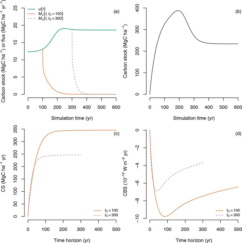
C. A. Sierra et al.: Climate benefit of sequestration                                                                               1031

   The AGWP can be computed for any other greenhouse gas               a pulse of 100 Gt of carbon to a pre-industrial atmosphere
using their respective radiative efficiencies and fate in the at-      with a background concentration of 280 ppm (PI100 func-
mosphere (impulse response function). To compare differ-               tion from here on), and another function was obtained by
ent gases, the global warming potential (GWP) is defined as            emitting 100 Gt of carbon to a present-day atmosphere with
the AGWP of a particular gas divided by the AGWP of CO2                a background of 389 ppm (PD100 from here on). The func-
(Shine et al., 1990; Lashof and Ahuja, 1990). Our interest in          tions they report are averages from the numerical output of
this paper is on carbon fixation and respiration in the form           multiple models fitted to a sum of exponential functions that
CO2 ; therefore, we primarily concentrate here on AGWP.                include an intercept term. This intercept implies that a pro-
   The impulse response function ha (t − t0 ) plays a central          portion of the added CO2 never leaves from the atmosphere–
role within the AGWP framework. The function encodes in-               ocean–terrestrial system to long-term geological reservoirs.
formation about the fate of a gas once it enters the atmo-             Following Millar et al. (2017), we added a timescale of 1 mil-
sphere and determines for how long the gas will remain.                lion years that corresponds to the intercept term in the IRFs.
Therefore, it can be interpreted as a density distribution for         The addition of this timescale has no effect on the results pre-
the transit time of a gas, since the time of emission until it         sented here, which are focused on much shorter timescales,
is removed by natural sinks (e.g., CO2 ) or by chemical reac-          but they avoid the mathematical problem that the integrals
tions (e.g., CH4 ).                                                    of the original functions go to infinity with time (Lashof and
   The function typically is assumed to be static; i.e., the time      Ahuja, 1990; Millar et al., 2017).
at which the gas enters the atmosphere is not relevant, only
the time it remains there (t − t0 ). However, this function can        2.3   Carbon sequestration CS and the climate benefit of
be time-dependent, expressing different shapes depending on                  carbon sequestration (CBS)
the time the gas enters the atmosphere, i.e., ha (t0 , t − t0 ). For
example, when natural sinks saturate, faster accumulation of           GWPs are useful to quantify the climate impacts of increas-
CO2 and longer transit times of carbon in the atmosphere               ing or reducing emissions of GHGs to the atmosphere. How-
are observed (Metzler et al., 2018). In this situation, the spe-       ever, it is also necessary to quantify the climate benefits of
cific time of an emission would lead to different response             carbon flows in the opposite direction, atmosphere → land.
functions in the atmosphere. Because current research on im-           Furthermore, it is also important to quantify not only how
pulse response functions primarily considers the static time-          much and how fast carbon enters ecosystems, but also for
independent case (see Millar et al., 2017, for an exception),          how long the carbon stays (Körner, 2017).
we will consider only the static case for the remainder of this           Carbon taken up from the atmosphere through the process
paper.                                                                 of photosynthesis is stored in multiple ecosystem reservoirs
                                                                       for a particular amount of time. Carbon sequestration can be
2.2   The radiative efficiency of CO2 and its impulse                  defined as the process of capture and long-term storage of
      response function                                                CO2 (Sedjo and Sohngen, 2012). We define here carbon se-
                                                                       questration CS over a time horizon T as
The radiative efficiency of CO2 is a function of the concen-                                 tZ
                                                                                              0 +T
tration of this gas and the concentration of other gases in the        CS(T , S0 , t0 ) :=           Ms (t − t0 ) dt,                 (5)
atmosphere with overlapping absorption bands (Lashof and
                                                                                             t0
Ahuja, 1990; Shine et al., 1990). Therefore, kCO2 changes as
the concentration of GHGs change in the atmosphere. For                where Ms (t − t0 ) represents the fate of a certain amount of
most applications however, the radiative efficiency of CO2             carbon S0 taken up by the sequestering system at a time
has been assumed constant in the limit of a small pertur-              t0 . Notice that this definition of carbon sequestration is very
bation at a specific background concentration (Lashof and              similar to that of AGWP for an emission, with the exception
Ahuja, 1990; Shine et al., 1990; Joos et al., 2013; Myhre              that the radiative efficiency term is omitted.
et al., 2013).                                                             To obtain the fate of sequestered carbon over time, we
   Here, we use a constant value of kCO2 = 6.48 ×                      represent carbon cycling and storage in ecosystems using
10−12 W m−2 per megagram of carbon based on results re-                the theory of compartmental dynamical systems (Luo et al.,
ported by Joos et al. (2013) for an atmospheric background             2017; Sierra et al., 2018a). In their most general form, we
of 389 ppm (∼ present day). This radiative efficiency repre-           can write carbon cycle models as
sents the change in radiative forcing caused by a change of
                                                                       dx(t)
1 Mg of carbon in the atmosphere in the form of CO2 in units                 = ẋ(t) = u(x, t) + B(x, t) x,                           (6)
of rate of energy transfer (watt) per square meter of surface.          dt
   Joos et al. (2013) have also derived impulse response func-         where x(t) ∈ Rn is a vector of n ecosystem carbon pools,
tions (IRFs) of CO2 in the atmosphere using coupled carbon–            u(x, t) ∈ Rn is a time-dependent vector-valued function of
climate models that include multiple feedbacks among Earth             carbon inputs to the system, and B(x, t) ∈ Rn×n is a time-
system processes. One function was obtained by emitting                dependent compartmental matrix. The latter two terms can

https://doi.org/10.5194/bg-18-1029-2021                                                               Biogeosciences, 18, 1029–1048, 2021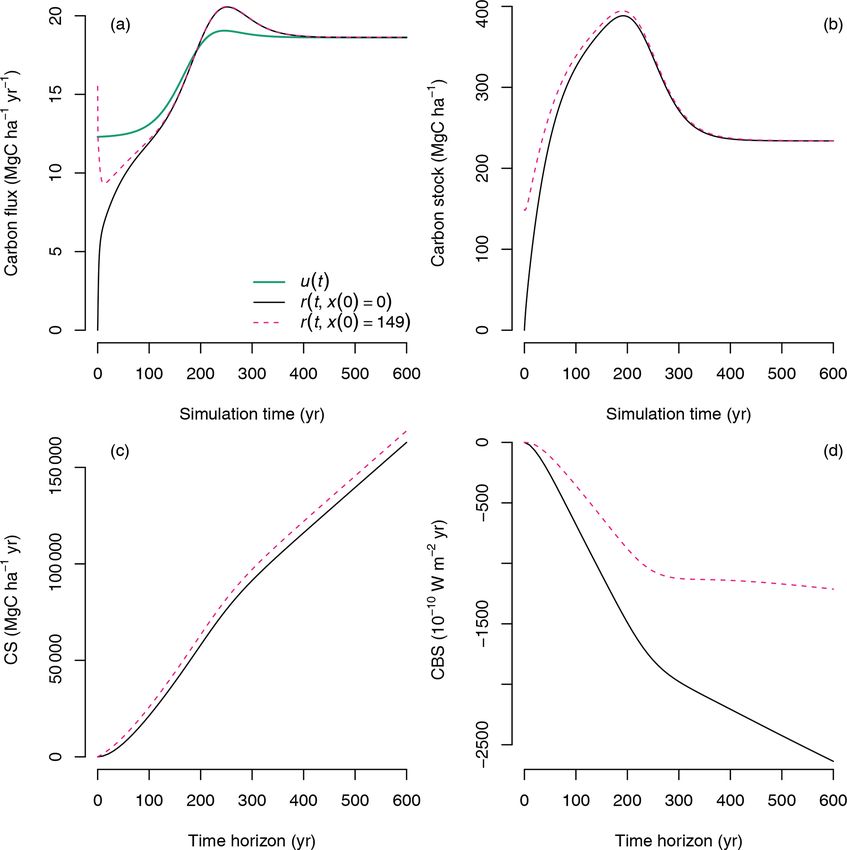
1032                                                                        C. A. Sierra et al.: Climate benefit of sequestration

depend on the vector of states, in which case the compart-              For the atmosphere, carbon sequestration is a form of neg-
mental system is considered nonlinear. In case the input vec-        ative emission, and we can represent its fate in the atmo-
tor and the compartmental matrix have fixed coefficients (no         sphere as
time dependencies), the system is considered autonomous,
and it is considered non-autonomous otherwise (Sierra et al.,                                           Zt
2018a). This distinction of models with respect to linearity         Ma0 (t) = −ha (t − t0 )S0 +             ha (t − τ )r(τ ) dτ,   (10)
and time dependencies (autonomy) is fundamental to dis-                                                 t0
tinguish important properties of models. For instance, mod-
els expressed as autonomous linear systems have a steady-            where the prime symbol represents a perturbed atmosphere
state solution given by x ∗ = −B−1 u, where x ∗ is a vec-            as an effect of sequestration. The first term in the right-hand
tor of steady-state contents for all ecosystem pools. Non-           side represents the response of the atmosphere to an instanta-
autonomous models have no steady-state solution.                     neous sequestration S0 at t0 , and the second term represents
   The fate of the fixed carbon for the general nonlinear non-       the perturbation in the atmosphere of the carbon returning
autonomous case can be obtained as                                   back from the terrestrial biosphere. Notice that the integral
                                                                     in this equation can be written as a convolution (ha ? r)(t)
Ms (t − t0 ) =k 8(t, t0 )β(t0 )S0 k,                          (7)    between the impulse response function of atmospheric CO2
                                                                     and the carbon returning from ecosystems to the atmosphere.
where β(t0 )S0 = u(t0 ), and β(t0 ) is an n-dimension vector
                                                                        We define now the climate benefit of sequestration for a
representing the partitioning of the total sequestered carbon
                                                                     pulse of CO2 into an ecosystem as
among n ecosystem carbon pools (Ceballos-Núñez et al.,
2020). The n × n matrix 8(t, t0 ) is the state-transition opera-                             tZ
                                                                                              0 +T
tor, which represents the dynamics of how carbon moves in a
                                                                     CBS(T , S0 , t0 ) :=            kCO2 Ma0 (t) dt,
system of multiple interconnected compartments (see details
in Appendix B). Throughout this document, we use the sym-                                    t0
bol k k to denote the 1-norm of a vector, i.e., the sum of the                     tZ
                                                                                    0 +T
absolute values of all elements in a vector.                            = −kCO2            (ha (t − t0 )S0 − (ha ? r)(t)) dt.       (11)
   Because ecosystems and most reservoirs are open systems,
                                                                                    t0
the sequestered carbon S0 returns back to the atmosphere,
mostly as CO2 due to ecosystem respiration and fires. Carbon         This metric integrates over a time horizon T the radiative
release r(t) from ecosystems can be obtained according to            effect avoided by sequestration of an amount of carbon S0
                                                                     taken up at time t0 by an ecosystem. It captures the timescale
r(t) = −1| B(t)8(t, t0 )β(t0 )S0 ,                            (8)
                                                                     at which the carbon is stored and gradually returns back to
where 1| is the transpose of the n-dimensional vector con-           the atmosphere. It can also be interpreted as the atmospheric
taining only 1s. The state-transition matrix captures the en-        response to carbon sequestration in the form of a negative
tire fate and dynamics of the sequestered carbon, from the           emission of CO2 during a time horizon of interest. It relies
time it enters t0 until release at any t.                            on knowledge of the atmospheric response to perturbations
   The link between the time it takes sequestered carbon S0 to       in the form of an impulse response function and the transit
appear in the release flux r(t) is established by the concept of     time of carbon in an ecosystem.
transit time (Metzler et al., 2018). In particular, we define the
forward transit time (FTT) as the age that fixed carbon will         2.4   Ecosystems in equilibrium: the linear, steady-state
have at the time it is released back to the atmosphere, or how             case
long a mass fixed now will stay in the system. The backward
transit time (BTT) is defined as the age of the carbon in the        The computation of CS and CBS is simplified for systems
output flux since the time it was fixed, or how long the mass        in equilibrium. For linear systems at a steady state, the time
leaving the system now had stayed. This implies that                 at which the carbon enters the ecosystem is irrelevant (Kloe-
                                                                     den and Rasmussen, 2011; Rasmussen et al., 2016); one only
r(t) = pBTT (t − t0 , t) = pFTT (t − t0 , t0 ),               (9)    needs to know for how long the carbon has been in the sys-
                                                                     tem to predict how much of it remains. Mathematically, this
where pBTT (t − t0 , t) is the backward transit time distribu-       implies
tion of carbon leaving the system at time t with an age t − t0 ,
while pFTT (t − t0 , t0 ) is the forward transit time distribution   8(t, t0 ) = ea·B for all t0 ≤ t and a = t − t0 .               (12)
of carbon entering the system at time t0 and leaving with
an age t − t0 . For systems in equilibrium, both quantities are      Therefore, for linear systems at a steady state, we have the
equal (Metzler et al., 2018). For systems not in equilibrium,        special cases
semi-explicit formulas for their distributions are given in Ap-
pendix B.                                                            Ms (a) = kea·B uk,                                             (13)

Biogeosciences, 18, 1029–1048, 2021                                                         https://doi.org/10.5194/bg-18-1029-2021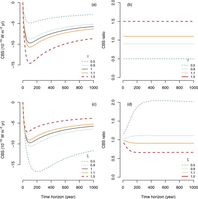
C. A. Sierra et al.: Climate benefit of sequestration                                                                                  1033

Figure 1. Contrast between current approach to quantification of climate effects of emissions and sequestration (a), and the proposed ap-
proach for sequestration (b). Plots and equations represent the concepts of absolute global warming potential (AGWP) of an emission of
CO2 , carbon sequestration (CS), and climate benefits of sequestration (CBS). AGWP integrates over a time horizon T the fate of an instant
emission at time t0 of a gas (Ma (t)) and multiplies by the radiative efficiency k of the gas. A similar idea can be used to define CS as
the integral of the fate Ms (t) of an instant amount of carbon uptake S0 over T . The CBS captures the atmospheric disturbance caused by
CO2 uptake and subsequent release by respiration as the integral over T of the fate of sequestered carbon Ma0 (t) multiplied by the radiative
efficiency of CO2 .

and                                                                         Furthermore, it is possible to find a closed-form expression
                        u                                                for this integral:
Ms1 (a) = ea·B             ,                                   (14)
                       kuk
                                                                         CS(T ) = kB−1 eT ·B − I uk,                                (19)
where Ms1 represents the fate of one unit of fixed carbon,
which can also be interpreted as the proportion of carbon re-            where I ∈ Rn×n is the identity matrix. Similarly, for one unit
maining after the time of fixation.                                      of carbon entering a steady-state system at any time, we de-
   The amount of released carbon returning to the atmosphere             fine CS1 as
is therefore
r(a) = −1| B ea·B u,                                           (15)                   ZT
                                                                                                   u
which for one unit of fixed carbon is equal to the transit               CS1 (T ) =        ea·B         da,                             (20)
                                                                                                  kuk
time density distribution f (τ ) of a linear system (Metzler                          0
and Sierra, 2018, see also Appendix B)
                                                                         which by integration gives
                            u
r1 (a) = −1| B ea·B            ,                               (16)
                           kuk                                                                   u
                                                                         CS1 (T ) = B−1 eT ·B − I     .                                 (21)
where r1 (a) = f (τ ), with mean (expected value) transit time                                    kuk
given by
                                                                            These steady-state expressions can be very useful to com-
               |    −1    u    kx ∗ k                                    pare different systems or changes to a particular system if
E(τ ) = −1 B                 =        .                        (17)
                         kuk   kuk                                       the steady-state assumption is justified. Furthermore, it can
                                                                         be shown that in the long term, as the time horizon T goes to
  We can now derive the steady-state expression of CS as
                                                                         infinity (∞), the term (eT ·B − I) converges to −I, and there-
           ZT                                                            fore Eq. (19) converges to the expression
CS(T ) =           kea·B uk da.                                (18)
                                                                          lim CS(T ) = kx ∗ k,                                          (22)
           0                                                             T →∞

https://doi.org/10.5194/bg-18-1029-2021                                                            Biogeosciences, 18, 1029–1048, 2021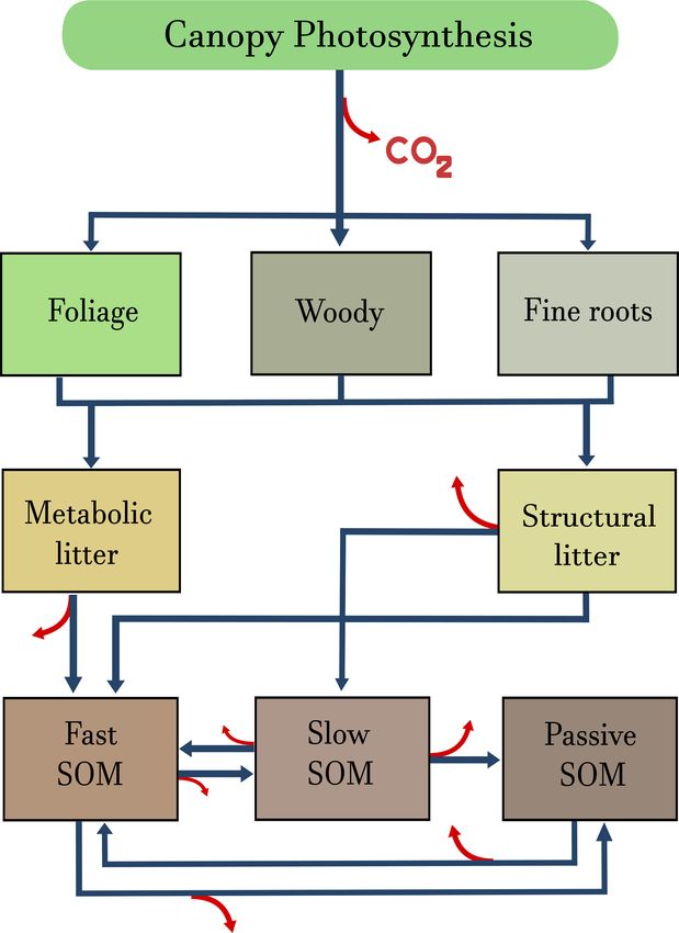
1034                                                                                     C. A. Sierra et al.: Climate benefit of sequestration

which means that the total amount of carbon at a steady state
is equal to the long-term carbon sequestration of an instanta-                                        tZ
                                                                                                       0 +T
neous amount of fixed carbon at an arbitrary time.
                                                                                 CBS(T , s, t0 ) :=           kCO2 Ma0 (t) dt,
   Similarly, for one unit of carbon entering a system at a
steady state, the long-term CS1 from Eq. (21) can be obtained                                         t0
simply as                                                                                                       tZ
                                                                                                                 0 +T

                                                                                                = −kCO2               (ha ? (s − r))(t) dt.   (28)
 lim CS1 (T ) = E(τ )                                                     (23)
T →∞                                                                                                             t0

by using the definition of mean transit time of Eq. (17). This                   This expression of CBS accounts for the dynamic behavior
means that long-term sequestration of one unit of CO2 con-                       of inputs and outputs of carbon in ecosystems, and it can be
verges to the mean transit time of carbon in an ecosystem.                       used to represent time dependencies resulting from environ-
                                                                                 mental changes and disturbances or produced by emission
2.5    Dynamic ecosystems out of equilibrium: the                                scenarios or scheduled management activities. This time-
       continuous sequestration and emissions case                               dependent CBS is computed for a time horizon T starting at
                                                                                 any initial time t0 . In other words, it can be used to analyze
In addition of considering isolated pulses of emissions E0 or                    specific time windows of interest, accounting for the fate of
sequestrations S0 , we can also consider permanently ongoing                     all carbon sequestered during specific time intervals.
emissions e : t 7 −→ E(t) and sequestration s : t 7 −→ S(t), re-
spectively. Hence,
                                                                                 3     Example 1: CS and CBS for linear systems in
                        tZ
                         0 +T                                                          equilibrium
CS(T , s, t0 ) :=               Ms (t) dt,                                (24)
                                                                                 3.1    The fate of a pulse of inputs through the system
                         t0

where                                                                            A simple ecosystem carbon model, the terrestrial ecosystem
                                                                                 model (TECO), will now demonstrate an application of the
           Zt                                                                    theory to compute CS and CBS assuming a linear system at
Ms (t) =            k8(t, τ ) β(τ ) s(τ )k dτ.                            (25)   a steady state (i.e., in equilibrium). We used a modified ver-
           t0                                                                    sion of the TECO model, originally described by Weng and
                                                                                 Luo (2011) with parameter values obtained through data as-
   Here s(τ ) is a scalar flux of sequestration at time τ . This                 similation using observations from the Duke Forest in North
leads to                                                                         Carolina, USA. It contains eight main compartments: foliage
                                                                                 x1 , woody biomass x2 , fine roots x3 , metabolic litter x4 ,
                          Zt
                |                                                                structural litter x5 , fast soil organic matter (SOM) x6 , slow
r(t) = −1 B(t)                 8(t, τ ) β(τ ) s(τ ) dτ.                   (26)   SOM x7 , and passive SOM x8 (Fig. 2). The model represents
                         t0                                                      the dynamics of carbon at a temperate forest dominated by
                                                                                 loblolly pine. We chose this model due to its simplicity and
   The fate of sequestered carbon, for the atmosphere in the
                                                                                 tractability, but the framework presented in Sect. 2 can be ap-
form of a balance between simultaneous sequestration and
                                                                                 plied to more complex models and for other ecosystems (see
return of carbon, can now be obtained as
                                                                                 reference in Sect. “Executable research compendium (ERC)”
                Zt                             Zt                                for an example with a nonlinear model). In addition to its
Ma0 (t) = −           ha (t − τ ) s(τ ) dτ +        ha (t − τ )r(τ ) dτ          simplicity and tractability, there are two advantages of us-
                                                                                 ing this model over others: (1) it provides reasonable predic-
                t0                             t0
                                                                                 tions of net ecosystem carbon fluxes and biometric pool data
                Zt                                                               (Weng and Luo, 2011); (2) it is commonly used to express
        =−            ha (t − τ ) [s(τ ) − r(τ )] dτ                             complex ecosystem-level concepts such as the matrix gener-
                t0                                                               alization of carbon cycle models, their traceability, and tran-
        = −(ha ? (s − r))(t).                                             (27)   sient behavior (e.g., Luo and Weng, 2011; Luo et al., 2012;
                                                                                 Xia et al., 2013; Luo et al., 2017; Sierra, 2019).
We can now define the climate benefit of sequestration for a                        The model is commonly expressed as
dynamic ecosystem with continuous sequestration and respi-                       dX(t)
ration as                                                                              = bU (t) + ξ(t)ACX(t),                                 (29)
                                                                                  dt
                                                                                 where X is a vector of ecosystem carbon pools, C is a diag-
                                                                                 onal matrix with cycling rates for each pool, A is a matrix of

Biogeosciences, 18, 1029–1048, 2021                                                                   https://doi.org/10.5194/bg-18-1029-2021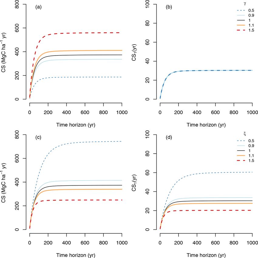
C. A. Sierra et al.: Climate benefit of sequestration 1035
Figure 2. Graphical representation of the terrestrial ecosystem
model (TECO) described in Weng and Luo (2011) and Luo et al.
(2012). Carbon enters the ecosystem through canopy photosynthe- Figure 3. Fate of carbon (Ms (t), left axis; and Ms1 (t), right axis)
sis and is allocated to three biomass pools: foliage, woody biomass, entering the ecosystem according to the TECO model parameter-
and fine roots. From these pools, carbon is transferred to metabolic ized for the Duke Forest and calculated using Eq. (13) for the upper
and structural litter pools, from where it can be respired as CO2 or panel, and respired carbon (r(t)) returning back to the atmosphere
transferred to the soil organic matter (SOM) pools. Blue arrows rep- calculated using Eq. (15).
resent transfers among compartments, and red arrows release to the
atmosphere in the form of CO2 .
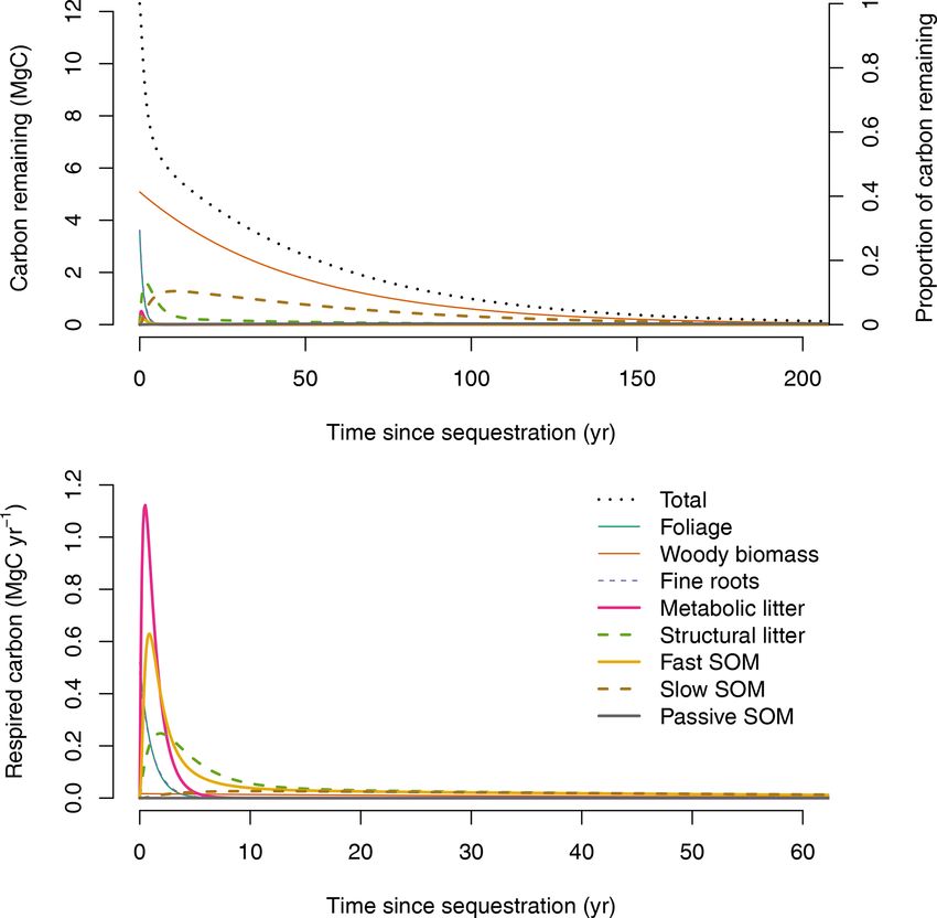
carbon is returned back to the atmosphere in 7.6 years and
transfer coefficients among pools, and b is a vector of alloca- 95 % in 124 years.
tion coefficients to plant parts. We modified the entries of ma- Ecosystem-level CS, i.e., the area under the curve of the
trix A to allow autotrophic respiration to be computed from amount of remaining carbon over time (area under dotted
the vegetation pools and not from the GPP flux as in the orig- line in Fig. 3, upper panel), increases towards an asymp-
inal model (see details in Appendix C). The function U (t) tote as the time horizon of integration increases (Fig. 4a).
determines the carbon inputs to the system as gross primary Here, CS is reported in units of Mg C ha−1 yr, because
production (GPP), and ξ(t) is a time-dependent function that this is the amount of carbon retained in organic matter
modifies ecosystem cycling rates according to changes in the over a fixed time horizon. For relevant time horizons of
environment. 50, 100, 500, and 1000 years, CS was 233.51, 317.68,
For this steady-state example, we assume constant in- 371.64, and 373.42 Mg C ha−1 yr, respectively. In the long
puts (U (t) = U ) and constant rates (ξ(t) = 1). Furthermore, term (i.e., as the time horizon goes to infinity), CS converges
defining B := AC, and u := bU , we can write this model as to the steady-state carbon stock predicted by the model of
a linear, autonomous compartmental system of the form 373.67 Mg C ha−1 .
A similar computation can be made for one unit of fixed
ẋ = u + B x, (30)
carbon (CS1 ). In this case CS1 was 18.98, 25.83, 30.21,
with values for B and u as described in Appendix C. and 30.36 years for time horizons of 50, 100, 500, and
The fate of a pulse of carbon input entering the ecosys- 1000 years, respectively. In the long term, CS1 converges to
tem at an arbitrary time when the system is in equilibrium the mean transit time of carbon: 30.4 years (Fig. 4b).
can be obtained by applying Eqs. (13) and (14) (Fig. 3). Car- Due to sequestration at t0 , the CBS shows a rapid neg-
bon enters the ecosystem through foliage, wood, and fine- ative increase in radiative forcing, which decreases as the
root pools. A large proportion of this carbon is quickly trans- time horizon increases due to the return of carbon to the at-
ferred from these pools to the fine and metabolic litter pools. mosphere as an effect of respiration (Fig. 4c). The shape of
Subsequently, the carbon moves to the SOM pools with im- the curve, however, depends strongly on the IRF for atmo-
portant respiration losses during these transfers. Most carbon spheric CO2 . CBS is larger over the long term (> 200 years)
is returned back to the atmosphere with a mean transit time for the present-day (PD100) curve proposed by Joos et al.
of 30.4 years for the whole system. Half of the sequestered (2013) than for the pre-industrial curve (PI100). During the
https://doi.org/10.5194/bg-18-1029-2021 Biogeosciences, 18, 1029–1048, 2021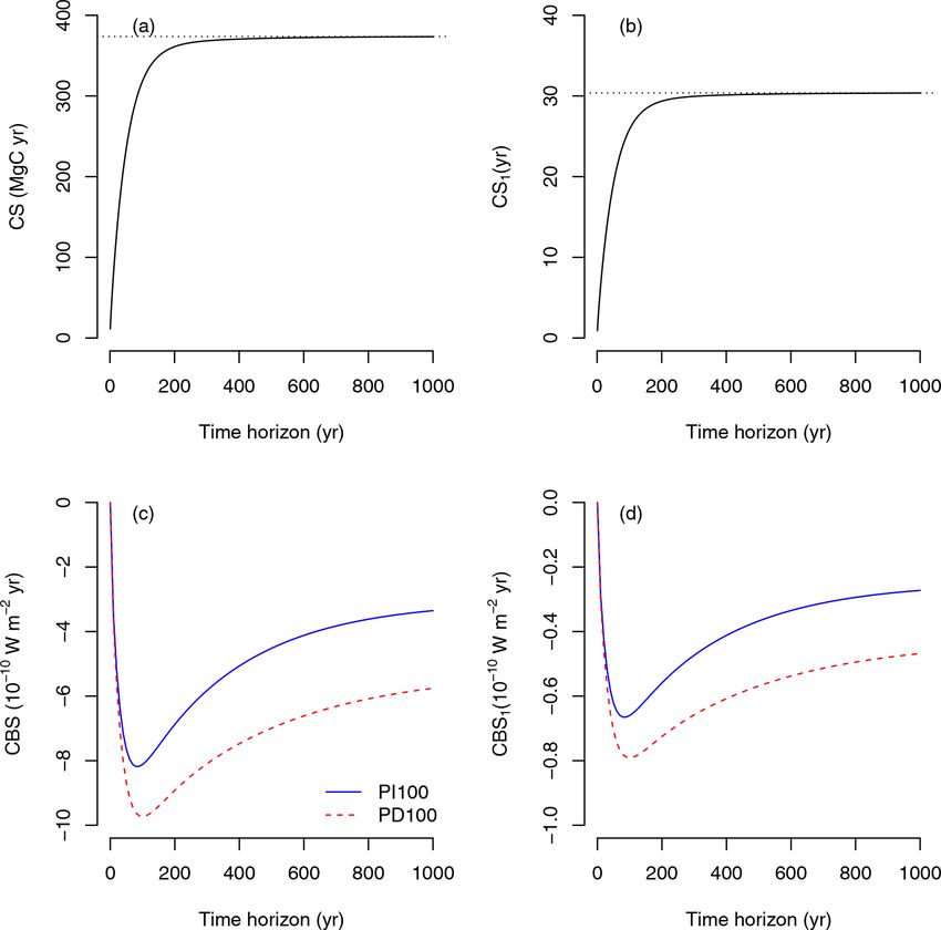
1036                                                                           C. A. Sierra et al.: Climate benefit of sequestration

                                                                        Figure 5. Absolute global warming potential (AGWP) due to the
                                                                        emission of 1 Mg of CO2 –C to the atmosphere for the two different
                                                                        IRFs (pre-industrial atmosphere with a pulse of 100 Gt of carbon:
                                                                        PI100, and present-day atmosphere with a pulse of 100 Gt of car-
                                                                        bon: PD100) reported by Joos et al. (2013).
Figure 4. Carbon sequestration (CS) and climate benefit of seques-
tration (CBS) for instantaneous carbon uptake at any given time.
(a) CS due to the uptake of 12.3 Mg C ha−1 , which corresponds to
GPP of 1 year. (b) CS due to the uptake of one unit of carbon (CS1 ).   corresponding to the amount of GPP sequestered in 1 year
(c) CBS due to the uptake of 12.3 Mg C ha−1 for two different im-       (12.3 Mg C ha−1 yr−1 for Duke Forest).
pulse response functions (pre-industrial atmosphere with a pulse of        In our example, the emission of 1 Mg of carbon to the at-
100 Gt of carbon: PI100, and present-day atmosphere with a pulse        mosphere has a predominant warming effect that cannot be
of 100 Gt of carbon: PD100). (d) CBS due to the uptake of one unit      compensated for by the sequestration of 1 Mg of carbon at
of carbon (CBS1 ) for two different impulse response function. Dot-     the Duke Forest (Fig. 6). However, the sequestration of the
ted lines in (a) and (b) represent steady-state carbon storage and      equivalent of GPP in 1 year can have a significant climate
mean transit time, respectively.                                        benefit compared to the emission of 1 Mg of carbon, depend-
                                                                        ing on the time horizon of analysis. When one integrates in
                                                                        time horizons lower than 200 years, CBS outweighs AGWP
pre-industrial period, perturbations of CO2 in the atmosphere           in this example. However, because the lifetime of an emis-
are lower than in the present-day period due to higher up-              sion of CO2 is much longer in the atmosphere than the transit
take of carbon from the oceans and the land biosphere (Joos             time of carbon through a forest ecosystem, AGWP outweighs
et al., 2013). Therefore, the benefits of carbon sequestration          CBS on longer timescales.
are larger under present-day conditions based on these IRF                 The time of integration in the computation of GWP has
curves. Impulse response functions depend strongly on the               been a heavily debated topic in the past, and this is related
magnitude and timing of the pulse (Joos et al., 2013; Mil-              to the topic of “permanence” of sequestration in carbon ac-
lar et al., 2017). Therefore, estimates of climate impacts of           counting and climate policy (Moura Costa and Wilson, 2000;
emissions (AGWP, Fig. 5) and climate benefits of sequestra-             Noble et al., 2000; Sedjo and Sohngen, 2012). One problem
tion (CBS, Fig. 4c, d) depend strongly on the choice of the             in these previous debates is that the timescale of carbon in
IRF. For the purpose of this paper, we will use the present-            ecosystems was not considered explicitly while the timescale
day curve (PD100) from here on.                                         of carbon in the atmosphere was. With the approach proposed
   Because AGWP and CBS are based on similar concepts                   here, both are explicitly taken into account and can better in-
and share similar units, it becomes possible to directly com-           form management and policy debates about sequestration of
pare one another (Fig. 6) and obtain an estimate of the cli-            carbon in natural and man-made sinks.
mate impact of emissions versus sequestration. This can be
done either as the ratio of the absolute value of CBS to                3.2   Carbon management to maximize the climate
AGWP, i.e., |CBS|/AGWP (unitless), or as the net radiative                    benefit of carbon sequestration
balance CBS + AGWP (W m−2 yr). It is possible to compute
these relations using the CBS for one unit of sequestered               In the context of climate change mitigation, management of
carbon, which provides a direct estimate of the impact of               ecosystems may be oriented to increase carbon sequestration
one unit of sequestration versus one unit of emission, or               and its climate benefit. In the recent past, scientists and pol-

Biogeosciences, 18, 1029–1048, 2021                                                        https://doi.org/10.5194/bg-18-1029-2021
C. A. Sierra et al.: Climate benefit of sequestration 1037
Both the transit time distribution (Eqs. B4 and 16) and the
mean transit time (Eq. 17) only take into account the propor-
tional distribution of the carbon inputs to the different pools
(u/kuk) but not the total amount of inputs. Therefore, a unit
of carbon that enters an ecosystem stays there for the same
amount of time independent of how much carbon is entering
the system. Although these results only apply to linear sys-
tems at a steady state, they provide some intuition about what
might be the case in systems out of equilibrium.
Carbon management can also be oriented to modify pro-
cess rates in ecosystems as encoded in the matrix B. A pro-
portional decrease in process rates by a factor ξ < 1 not only
increases carbon storage as
1
−(ξ B)−1 u = (−B−1 u),
ξ
x∗
= , (33)
ξ
Figure 6. Relations between CBS and AGWP for the IRF PD100 as but also increases the mean transit time as
a function of time horizon T . (a) Ratio between the absolute value
u E(τ )
of CBS and AGWP, based on a total sequestration of 12.3 Mg of −1| (ξ B)−1 = . (34)
carbon (back line, GPP equivalent for 1 ha and 1 year at Duke For- kuk ξ
est) versus a sequestration of 1 Mg of carbon (dashed green line).
(b) Radiative balance (net difference) between CBS and AGWP for A proportional change in the opposite direction (ξ > 1)
the sequestration of 12.3 Mg of carbon (black line) and 1 Mg of car- causes the opposite effect; a proportional increase in pro-
bon (dashed green line). cess rates decreases carbon storage and decreases mean tran-
sit time.
Based on these results, it is now clear that carbon man-
icy makers have advocated increasing the amount of inputs to agement to increase carbon inputs alone can only increase
ecosystems as an effective form of carbon management (e.g., CS but not CS1 ; i.e., the new carbon inputs have a sequestra-
Silver et al., 2000; Grace, 2004; Lal, 2004; Chabbi et al., tion benefit only through increase of carbon storage but not
2017; Minasny et al., 2017). Although increases in carbon through a longer transit time in ecosystems. Management to
inputs can increase the amount of stored carbon in an ecosys- decrease process rates, on the contrary, can increase both CS
tem with related climate benefits, it does not necessarily in- and CS1 because the new carbon entering the system stays
crease the amount of time the sequestered carbon will stay in there for longer.
the system. Therefore, strategies that focus on increasing car- We can see these effects of carbon management on CS by
bon inputs alone do not take full advantage of the potential running simulations using the TECO model at a steady state
of ecosystems to mitigate climate change. (Fig. 7). Now, we modified carbon inputs and process rates
We can conceptualize any management activity that in- by either increasing them by 10 % and 50 % (γ , ξ = 1.1, 1.5)
creases or reduces carbon inputs to an ecosystem by a factor or decreasing them by 10 % and 50 % (γ , ξ = 0.9, 0.5). The
γ , so the new inputs are given by the product γ u. For exam- simulations showed that increasing or decreasing carbon in-
ple, if we increase carbon inputs to an ecosystem by 10 %, puts increase or decrease CS for any time horizon (Fig. 7a),
γ = 1.1. Increasing carbon inputs by a proportion γ > 1 in- but it does not modify the behavior of one unit of sequestered
creases carbon storage at a steady state by an equal propor- carbon (CS1 ) (Fig. 7b). On the contrary, decreasing or in-
tion since creasing process rates increase or decrease both CS (Fig. 7c)
−B−1 (γ u) = γ (−B−1 u), and CS1 (Fig. 7d).
= γ x∗. (31) The resultant effects of changes in management of inputs
or process rates on CBS can differ substantially. Increases or
Similarly, a decrease in carbon inputs by a proportion γ < 1 decreases of carbon inputs have similar proportional effects
decreases steady-state carbon storage by an equal propor- on CBS, but differences in processes rates are not equally
tion. However, the time carbon requires to travel through the proportional. While an increase in inputs by 50 % would in-
ecosystem is still the same since the transit time does not crease CBS by 50 %, a decrease in process rates by 50 %
change, as we can see from the mean transit time expression would have an increase in CBS by more than 100 % for time
γu horizons longer than 300 years (Fig. 8). Similarly, while a
−1| B−1 = E(τ ). (32) decrease in inputs by 50 % would reduce CBS by 50 %, an
kγ uk
https://doi.org/10.5194/bg-18-1029-2021 Biogeosciences, 18, 1029–1048, 20211038 C. A. Sierra et al.: Climate benefit of sequestration
Figure 7. Different carbon management strategies and their effect Figure 8. Effects of different management strategies on CBS.
on the CS and CS1 . Management to increase or decrease carbon (a) Effect of increasing or decreasing carbon inputs by a proportion
inputs in the vector u by specific proportions γ is shown in panel (a) γ on CBS; (b) same effect of γ expressed as a ratio with respect to
and (b). Management to increase or decrease process rates in the the reference case of γ = 1. (c) Effects of decreasing or increasing
matrix B by a proportion ξ is shown in panels (c) and (d). Since CS1 process rates in the matrix B by a proportion ξ on CBS; (d) same
quantifies carbon sequestration of one unit of carbon, management effect of ξ expressed as a ratio with respect to the reference case
of the amount of carbon inputs does not modify CS1 in panel (b), ξ = 1.
and all lines overlap.
larger or smaller depending on the ecosystems being com-
pared).
increase in process rates by 50 % would decrease CBS by
only ∼ 40 %.
4 Example 2: CS and CBS for dynamic systems out of
These results show that management of transit time, e.g.,
equilibrium
by decreasing process rates, may lead to stronger climate
benefits than managing carbon inputs alone. Furthermore, 4.1 Pulses entering at different times and experiencing
one could think about optimization scenarios in which both different environments
inputs and transit times are managed to achieve larger cli-
mate benefits given certain constraints. The concept of CBS The steady-state examples above are useful to gain some in-
is thus a useful mathematical framework to formally pose tuition about potential long-term patterns in CS and CBS, but
such an optimization problem. for real-world applications it is necessary to consider systems
We can also use these results to infer differences in CS out of equilibrium and driven by specific time-dependent sig-
and CBS for different ecosystem types. Without manage- nals. We will consider now the case of the temperate ecosys-
ment, we would expect large variability of CS and CBS in tem of our previous example driven by increases in atmo-
the terrestrial biosphere. Inputs and process rates vary con- spheric CO2 concentrations that lead to higher photosyn-
siderably for terrestrial ecosystems as previously reported in thetic uptake and increasing temperatures that lead to faster
other studies. For instance, gross primary productivity can cycling rates. We will thus consider a non-autonomous ver-
range from about 1 to > 30 Mg C ha−1 yr−1 from high- to sion of the TECO model that follows the general form
low-latitude ecosystems (Jung et al., 2020). Based on simula-
tions from the CABLE model, Lu et al. (2018) found a range ẋ(t) = γ (t) · u + ξ(t) · B · x(t), (35)
of mean transit times between 13 and 341 years from low-
to high-latitude ecosystems. These large ranges of variability where the time-dependent function γ (t) incorporates the ef-
for GPP and mean transit time suggest that CS and CBS may fects of temperature and atmospheric CO2 on primary pro-
vary among ecosystems by large proportions (> 20 times duction, and the function ξ(t) incorporates the effects of tem-
Biogeosciences, 18, 1029–1048, 2021 https://doi.org/10.5194/bg-18-1029-2021C. A. Sierra et al.: Climate benefit of sequestration 1039
Although more carbon enters the ecosystem at simulation
year 300 than at year 100 due to the CO2 fertilization effect, it
is lost much faster because of higher temperatures that result
in faster transit times for simulation times above 300 years
(Fig. 9a). The slower transit times experienced by the carbon
that enters at year 100 due to lower temperature result then in
much higher values of CS for time horizons T > 100 years
(Fig. 9c). Similarly for CBS, where differences are evident
much earlier, lower temperatures lead to higher values of
CBS for time horizons T > 50 years (Fig. 9d).
This simple example highlights the importance of time-
dependent transit times in determining CS and CBS. If
changes in climate lead to faster carbon processing rates, we
would thus expect carbon to transit faster through the ecosys-
tem, returning faster to the atmosphere, and therefore with
lower values for carbon sequestration and its climate benefit.
4.2 Continuous inputs into a changing environment
In the previous example, we considered the case of two sin-
gle pulses entering the ecosystem at different times under
Figure 9. Prediction of CS and CBS for a non-steady-state case changing environmental conditions during a simulation. A
with time-dependent inputs u(t) controlled by CO2 fertilization consolidated view can be obtained by taking all single pulses
and temperature and process rates controlled by temperature modi- and integrating them continuously in time to compute CS and
fied by a time-dependent factor ξ(t). (a) Predicted time-dependent CBS using Eqs. (24) and (28), respectively. In this case, CS
inputs u(t), and the fate of carbon entering the ecosystem at increases monotonically, and CBS decreases monotonically
simulation year 100 (Ms (t, t0 = 100)) and simulation year 300 with time horizon (Fig. 10, continuous black lines), which
(Ms (t, t0 = 300)). (b) Predicted carbon accumulation in the ecosys- is somewhat obvious because as the ecosystem accumulates
tem (k x(t) k) for the entire simulation period. (c) Carbon seques-
carbon, more of it is retained in the ecosystem and is isolated
tration for the amount of inputs entering at simulation years 100 and
from atmospheric radiative effects. However, this simulation
300 calculated for different time horizons T . (d) Climate benefit of
sequestration for carbon entering the ecosystem at simulation years only considers carbon that enters the ecosystem from the be-
100 and 300 integrated for different time horizons T . ginning of the simulation until the end of the time horizon,
from t0 to t0 + T . An important aspect to consider is the role
of carbon already present in the ecosystem at t0 .
perature on respiration rates. Specific shapes for these func- We will consider now the case of continuous sequestration
tions were taken from Rasmussen et al. (2016) and are de- and release of carbon with differences in the initial condi-
scribed in detail in Appendix C. When applied to the CASA tions in the simulation, which can vary according to land use
model in Rasmussen et al. (2016), these functions predicted changes. For example, when changing land use from agricul-
an increase in primary production and an increase in process ture to forest, or from natural forest to plantation, there are
rates, which resulted in a decrease in transit times over a sim- carbon legacies that have an influence on future carbon tra-
ulation of 600 years. jectories (Harmon et al., 1990; Janisch and Harmon, 2002;
We used the same simulation setup here starting from Sierra et al., 2012). These carbon legacies are usually dead
an empty system (x(0) = 0) and obtained similar results in biomass and detritus, which cause ecosystems to lose carbon
terms of primary production and transit times as in Ras- via decomposition before photosynthesis from new biomass
mussen et al. (2016). We used these simulation results to compensates for the losses. In these initial stages of recovery,
compute CS and CBS for carbon entering the ecosystem at ecosystems are usually net carbon sources, but they still may
different times during the simulation window. In particular, store more carbon than an ecosystem developing from bare
we considered the case of the amount of carbon sequestered ground.
at years 100 and 300 after the start of the simulation; i.e., The CS and CBS concepts can be very useful to com-
we considered the cases t0 = 100 and t0 = 300 (Fig. 9a) and pare contrasting trajectories of ecosystem development and
computed the fate of this carbon (Ms (t, t0 , u0 )), its carbon assess their role in terms of carbon sequestration alone and
sequestration (CS(T , u0 , t0 )) and the climate benefit of se- their climate impact. For this purpose, we performed an ad-
questration (CBS(T , u0 , t0 )) for different time horizons T . ditional simulation in which at the starting time there is no
living biomass, but the detritus pools and the SOM pools
are 1.5 and 1.0 times as large as in the equilibrium case, re-
https://doi.org/10.5194/bg-18-1029-2021 Biogeosciences, 18, 1029–1048, 20211040 C. A. Sierra et al.: Climate benefit of sequestration
rics, these two different aspects of carbon sequestration can
be discussed separately.
5 Discussion
The metrics introduced here, carbon sequestration (CS) and
the climate benefit of sequestration (CBS), integrate both
the amount of carbon entering an ecosystem and the time
it is stored there, thus avoiding radiative effects in the at-
mosphere. Disproportionate attention is given to quantifying
sources and sinks of carbon in ongoing debates about the role
of ecosystems in climate change mitigation, with much less
attention paid to the fate of carbon once it enters an ecosys-
tem. The time carbon remains in an ecosystem, encapsulated
in the concept of transit time, is critical for climate change
mitigation because during this time carbon is removed from
radiative effects in the atmosphere.
The CS and CBS concepts unify atmospheric and ecosys-
tem approaches to quantifying the greenhouse effect. The
CBS concept builds on that of the absolute global warming
Figure 10. Computation of CS and CBS for continuous inputs and potential (AGWP) of a greenhouse gas. The main difference
release of carbon in simulations with different initial conditions x 0 : is that CBS quantifies avoided warming during the time car-
in one simulation the ecosystem develops from empty pools (x(0) = bon is stored in an ecosystem, while AGWP quantifies poten-
0, i.e., bare ground, black lines), and in the second simulation the tial warming when the carbon enters the atmosphere. Both
ecosystem develops from existing litter and SOM pools but empty metrics rely on the quantification of the fate of carbon (or
biomass pools (kx(0)k = 149.04 Mg C ha−1 , dashed magenta color other GHGs for AGWP) once it enters the particular system.
lines). (a) Inputs u(t) and release fluxes r(t) along the simulation For atmospheric systems, a significant amount of work has
time. (b) Carbon stocks predicted by the model along the simulation
been done in determining the fate of GHGs once they enter
time. (c) Carbon sequestration CS for a sequence of time horizons.
the atmosphere after emissions (e.g., Rodhe, 1990; O’Neill
(d) Climate benefit of sequestration CBS for a sequence of time
horizons. et al., 1994; Prather, 1996; Archer et al., 2009; Joos et al.,
2013). For terrestrial ecosystems; however, robust methods
to quantify the fate of carbon as it flows through terrestrial
system components have been developed only recently (Ras-
mussen et al., 2016; Metzler and Sierra, 2018; Metzler et al.,
spectively (kx(0)k = 149.04 Mg C ha−1 ). In this simulation, 2018).
the ecosystem losses a significant amount of carbon in the Global warming potential (GWP), or the climate impact
early stages of development, and respiration is much larger of an emission of a certain gas in relation to the impact
than primary production (r(t) > ku(t)k) (Fig. 10a, dashed of an emission of CO2 , is often used to assess climate im-
magenta line). Because soils are already close to an equilib- pacts of actions, e.g., avoided deforestation, land use change,
rium value, the ecosystem already has a large amount of car- and even enhanced carbon sequestration. However, this met-
bon stored; therefore in the computation of the fate of carbon ric has two limitations when applied to carbon sequestration
Ms (t, t0 ) there is already a larger amount of carbon to con- and in comparison to the combined use of CBS and AGWP
sider, which causes CS to be larger for the land-use-change we advocate here: (1) it only quantifies the climate effects of
case than for the bare ground case (Fig. 10c). On the con- emissions but not of sequestration and treats all fixed carbon
trary, because there are more emissions from the ecosystem equally independent of its transit time in the ecosystem and
in early development stages, CBS is lower for the land-use- (2) it is a relative measure with respect to the emission of
change case than for the bare ground case (Fig. 10d). CO2 . GWPs are commonly reported in units of CO2 equiv-
These contrasting results between CS and CBS for the alents, which only address indirectly the effect of a gas in
continuous case with contrasting initial conditions can be producing warming. In contrast, CBS quantifies the effects
very useful to address debates and controversies about the of avoided warming in units of W m−2 over the period of
role of land use change and baselines in carbon accounting. time carbon is retained.
The results show that carbon sequestration can still be high Other concepts have been proposed in the past to account
in ecosystems where emission fluxes are large, but climate for the temporary nature of carbon sequestration (see review
impacts can differ significantly. By using two different met- by Brandão et al., 2013, and references therein), with special
Biogeosciences, 18, 1029–1048, 2021 https://doi.org/10.5194/bg-18-1029-2021C. A. Sierra et al.: Climate benefit of sequestration 1041
interest in accounting for credits in carbon markets. In fact, TECO model is an excellent tool to illustrate ecosystem-level
“ton-year” accounting methods (Noble et al., 2000) resem- concepts because of its simplicity and tractability, but other
ble our definition of carbon sequestration; however, none of models with more accurate parameterizations and including
these previous concepts explicitly considers the time carbon more processes should be considered for practical applica-
is retained in the ecosystem. Instead, these approaches relate tions. The formulas and formal theory developed in Sect. 2
carbon sequestration to delay in fossil fuel emissions (Fearn- are general enough to deal with the non-steady-state case
side et al., 2000), or as the equivalence of the amount of as well as with models with nonlinear interactions among
carbon storage to AGWP (Moura Costa and Wilson, 2000). state variables. In Sierra (2020), we provide an example in
The concepts of sustained global warming potential (SGWP) the form of a Jupyter Notebook to compute CS and CBS
and sustained global cooling potential (SGCP) proposed by for a nonlinear model (see Sect. “Executable research com-
Neubauer and Megonigal (2015) are notable exceptions. The pendium (ERC)” for details).
CBS concept captures some of the ideas of the SGCP con- The concepts of CS and CBS present improvements to the
cept but differs in some fundamental assumptions related current guidelines for carbon inventories that treat all carbon
to the interpretation of the impulse response functions, the removals by sinks equally (IPCC, 2006) by explicitly con-
treatment of time-dependent fluxes and rates, and reporting. sidering the transit time of carbon in ecosystems. Therefore,
While SGCP reports values in reference to CO2 as is com- these new concepts have potential for being incorporated in
monly done for GWP, we report CBS for individual gases as revised policies for carbon accounting in the context of in-
it is done for AGWP. Appendix A elaborates on other aspects ternational climate agreements and carbon markets. CS and
of the SGWP and SGCP concepts. CBS can aid in the economic valuation of carbon by adding
The concept of CBS improves our ability to address some economic incentives to sequestration activities that retain car-
of the existing debates about the role of ecosystems in mit- bon in ecosystems for longer times. In addition, the concepts
igating climate change and enhances our potential to pro- can help in dealing with the issue of permanence of carbon by
vide decision support. In combination with quantifications of explicitly quantifying climate benefits of sequestration that
AGWP, CBS provides the net climate effect of an ecosystem can be compared directly with the climate impacts of emis-
or some management. For example, CBS can be used to bet- sions on a similar time horizon.
ter understand the climate impacts of storing carbon in long- Two potential limitations to apply the concepts of CS and
term reservoirs such as soils and wood products, as well as CBS are that they rely (1) on a model that tracks the fate of
the climate benefits of increasing the transit time in these sys- the fixed carbon and (2) on an impulse response function of
tems. CBS can be used to better quantify the climate benefits CO2 in the atmosphere. Reliable models may not be available
of using biofuels as fossil fuel substitution by computing the for certain types of ecosystems or may include large uncer-
CBS of the whole bioenergy production system and adding tainties that propagate to CS and CBS estimates. Also, es-
the negative AGWP attributed to the avoided emission. Sim- timates of impulse response functions for atmospheric CO2
ilarly, it can be incorporated in assessments of sequestration seem to also have uncertainties, particularly related to the
in industrial systems with associated carbon capture and stor- size of the emission pulse, the atmospheric background at
age. which the pulse is applied, and the long-term behavior of the
Carbon management of ecosystems can maximize CS curve for timescales longer than 1000 years (Archer et al.,
and/or CBS by not only increasing carbon inputs, but also by 2009; Lashof and Ahuja, 1990; Joos et al., 2013; Millar
increasing the transit time of carbon. There are many ways et al., 2017). However, one advantage of the functions pro-
in which the transit time of carbon can be increased – for posed by Joos et al. (2013) is that they are derived from cou-
instance, by increasing transfers of carbon to slow cycling pled climate–carbon models that include multiple feedbacks.
pools such as the case of increasing wood harvest allocation Therefore, when computing CS and CBS for small pertur-
to long-duration products (Schulze et al., 2019), or addition bations of the carbon cycle, it is not necessary to explicitly
of biochar to soils, or by reducing cycling rates of organic compute carbon–climate feedbacks. Also, when comparing
matter such as the case of soil flipping (Schiedung et al., two different systems with a CBS ratio as in Fig. (8) or a ra-
2019). Independently of the management activity, CS and tio CBS to AGWP (Fig. 6), uncertainties in the IRFs would
CBS can be powerful metrics to quantify their climate ben- tend to cancel each other out. Nevertheless, advances in our
efits, make comparisons among them, and compare against understanding of the fate of emitted CO2 to the atmosphere
baselines or no-management scenarios. will consequently derive better estimates of the climate ben-
The examples we provided in this paper illustrate the use efits of carbon sequestration.
and interpretation of CS and CBS metrics under the assump-
tions of linearity, steady state, or time dependencies in carbon
cycle dynamics with subsequent consequences for carbon se- 6 Conclusions
questration and its climate benefits. The computation of the
CBS relies on a model, which can be as simple as a one- Analyses of carbon sequestration for climate change mitiga-
pool model or a state-of-the-science land surface model. The tion purposes must consider both the amount of carbon in-
https://doi.org/10.5194/bg-18-1029-2021 Biogeosciences, 18, 1029–1048, 2021You can also read