Robust statistical calibration and characterization of portable low-cost air quality monitoring sensors to quantify real-time O3 and NO2 ...
←
→
Page content transcription
If your browser does not render page correctly, please read the page content below
Atmos. Meas. Tech., 14, 37–52, 2021
https://doi.org/10.5194/amt-14-37-2021
© Author(s) 2021. This work is distributed under
the Creative Commons Attribution 4.0 License.

Robust statistical calibration and characterization of portable
low-cost air quality monitoring sensors to quantify real-time O3
and NO2 concentrations in diverse environments
Ravi Sahu1 , Ayush Nagal2 , Kuldeep Kumar Dixit1 , Harshavardhan Unnibhavi3 , Srikanth Mantravadi4 , Srijith Nair4 ,
Yogesh Simmhan3 , Brijesh Mishra5 , Rajesh Zele5 , Ronak Sutaria6 , Vidyanand Motiram Motghare7 ,
Purushottam Kar2 , and Sachchida Nand Tripathi1
1 Department  of Civil Engineering, Indian Institute of Technology Kanpur, Kanpur, India
2 Department  of Computer Science and Engineering, Indian Institute of Technology Kanpur, Kanpur, India
3 Department of Computational and Data Sciences, Indian Institute of Science, Bengaluru, India
4 Department of Electrical Communication Engineering, Indian Institute of Science, Bengaluru, India
5 Department of Electrical Engineering, Indian Institute of Technology, Mumbai, India
6 Centre for Urban Science and Engineering, Indian Institute of Technology, Mumbai, India
7 Maharashtra Pollution Control Board, Mumbai, India

Correspondence: Sachchida Nand Tripathi (snt@iitk.ac.in)

Received: 3 April 2020 – Discussion started: 12 June 2020
Revised: 4 October 2020 – Accepted: 1 November 2020 – Published: 4 January 2021

Abstract. Low-cost sensors offer an attractive solution to        age point increase in terms of R 2 values offered by classi-
the challenge of establishing affordable and dense spatio-        cal non-parametric methods. We also offer a critical analysis
temporal air quality monitoring networks with greater mo-         of the effect of various data preparation and model design
bility and lower maintenance costs. These low-cost sensors        choices on calibration performance. The key recommenda-
offer reasonably consistent measurements but require in-          tions emerging out of this study include (1) incorporating
field calibration to improve agreement with regulatory instru-    ambient relative humidity and temperature into calibration
ments. In this paper, we report the results of a deployment       models; (2) assessing the relative importance of various fea-
and calibration study on a network of six air quality moni-       tures with respect to the calibration task at hand, by using an
toring devices built using the Alphasense O3 (OX-B431) and        appropriate feature-weighing or metric-learning technique;
NO2 (NO2-B43F) electrochemical gas sensors. The sensors           (3) using local calibration techniques such as k nearest neigh-
were deployed in two phases over a period of 3 months at          bors (KNN); (4) performing temporal smoothing over raw
sites situated within two megacities with diverse geographi-      time series data but being careful not to do so too aggres-
cal, meteorological and air quality parameters. A unique fea-     sively; and (5) making all efforts to ensure that data with
ture of our deployment is a swap-out experiment wherein           enough diversity are demonstrated in the calibration algo-
three of these sensors were relocated to different sites in the   rithm while training to ensure good generalization. These re-
two phases. This gives us a unique opportunity to study the       sults offer insights into the strengths and limitations of these
effect of seasonal, as well as geographical, variations on cal-   sensors and offer an encouraging opportunity to use them
ibration performance. We report an extensive study of more        to supplement and densify compliance regulatory monitor-
than a dozen parametric and non-parametric calibration al-        ing networks.
gorithms. We propose a novel local non-parametric calibra-
tion algorithm based on metric learning that offers, across de-
ployment sites and phases, an R 2 coefficient of up to 0.923
with respect to reference values for O3 calibration and up to
0.819 for NO2 calibration. This represents a 4–20 percent-

Published by Copernicus Publications on behalf of the European Geosciences Union.
38                       R. Sahu et al.: Robust statistical calibration and characterization of low-cost air quality sensors

1    Introduction                                                  1.1   Challenges in low-cost sensor calibration

Elevated levels of air pollutants have a detrimental impact        Measuring ground-level O3 and NO2 is challenging as they
on human health as well as on the economy (Chowdhury               occur at parts-per-billion levels and intermix with other pol-
et al., 2018; Landrigan et al., 2018). For instance, high levels   lutants (Spinelle et al., 2017). LCAQ sensors are not de-
of ground-level O3 have been linked to difficulty in breath-       signed to meet rigid performance standards and may gen-
ing, increased frequency of asthma attacks and chronic ob-         erate less accurate data as compared to regulatory-grade
structive pulmonary disease (COPD). The World Health Or-           CAAQMSs (Mueller et al., 2017; Snyder et al., 2013; Miskell
ganization reported (WHO, 2018) that in 2016, 4.2 million          et al., 2018). Most LCAQ gas sensors are based on ei-
premature deaths worldwide could be attributed to outdoor          ther metal oxide (MOx) or electrochemical (EC) technolo-
air pollution, 91 % of which occurred in low- and middle-          gies (Pang et al., 2017; Hagan et al., 2019). These present
income countries where air pollution levels often did not          challenges in terms of sensitivity towards environmental con-
meet its guidelines. There is a need for accurate real-time        ditions and cross-sensitivity (Zimmerman et al., 2018; Lewis
monitoring of air pollution levels with dense spatio-temporal      and Edwards, 2016). For example, O3 electrochemical sen-
coverage.                                                          sors undergo redox reactions in the presence of NO2 . The
   Existing regulatory techniques for assessing urban air          sensors also exhibit loss of consistency or drift over time.
quality (AQ) rely on a small network of Continuous Ambient         For instance, in EC sensors, reagents are spent over time and
Air Quality Monitoring Stations (CAAQMSs) that are instru-         have a typical lifespan of 1 to 2 years (Masson et al., 2015;
mented with accurate air quality monitoring gas analyzers          Jiao et al., 2016). Thus, there is a need for the reliable cali-
and beta-attenuation monitors and provide highly accurate          bration of LCAQ sensors to satisfy performance demands of
measurements (Snyder et al., 2013; Malings et al., 2019).          end-use applications (De Vito et al., 2018; Akasiadis et al.,
However, these networks are established at a commensu-             2019; Williams, 2019).
rately high setup cost and are cumbersome to maintain (Sahu
et al., 2020), making dense CAAQMS networks impractical.           1.2   Related works
Consequently, the AQ data offered by these sparse networks,
however accurate, limit the ability to formulate effective AQ      Recent works have shown that LCAQ sensor calibration
strategies (Garaga et al., 2018; Fung, 2019).                      can be achieved by co-locating the sensors with regulatory-
   In recent years, the availability of low-cost AQ (LCAQ)         grade reference monitors and using various calibration mod-
monitoring devices has provided exciting opportunities for         els (De Vito et al., 2018; Hagan et al., 2019; Morawska
finer-spatial-resolution data (Rai et al., 2017; Baron and         et al., 2018). Zheng et al. (2019) considered the problem
Saffell, 2017; Kumar et al., 2015; Schneider et al., 2017;         of dynamic PM2.5 sensor calibration within a sensor net-
Zheng et al., 2019). The cost of a CAAQMS system that              work. For the case of SO2 sensor calibration, Hagan et al.
meets federal reference method (FRM) standards is around           (2019) observed that parametric models such as linear least-
USD 200 000, while that of an LCAQ device running com-             squares regression (LS) could extrapolate to wider concentra-
modity sensors is under USD 500 (Jiao et al., 2016; Simmhan        tion ranges, at which non-parametric regression models may
et al., 2019). In this paper, we use the term “commodity” to       struggle. However, LS does not correct for (non-linear) de-
refer to sensors or devices that are not custom built and in-      pendence on temperature (T ) or relative humidity (RH), for
stead sourced from commercially available options. The in-         which non-parametric models may be more effective.
creasing prevalence of the Internet of things (IoT) infrastruc-       Since electrochemical sensors are configured to have
ture allows for building large-scale networks of LCAQ de-          diffusion-limited responses and the diffusion coefficients
vices (Baron and Saffell, 2017; Castell et al., 2017; Arroyo       could be affected by ambient temperature, Sharma et al.
et al., 2019).                                                     (2019), Hitchman et al. (1997) and Masson et al. (2015)
   Dense LCAQ networks can complement CAAQMSs to                   found that at RH exceeding 75 % there is substantial error,
help regulatory bodies identify sources of pollution and           possibly due to condensation on the potentiostat electronics.
formulate effective policies; allow scientists to model in-        Simmhan et al. (2019) used non-parametric approaches such
teractions between climate change and pollution (Hagan             as regression trees along with data aggregated from multi-
et al., 2019); allow citizens to make informed decisions,          ple co-located sensors to demonstrate the effect of the train-
e.g., about their commute (Apte et al., 2017; Rai et al., 2017);   ing dataset on calibration performance. Esposito et al. (2016)
and encourage active participation in citizen science initia-      made use of neural networks and demonstrated good calibra-
tives (Gabrys et al., 2016; Commodore et al., 2017; Gillooly       tion performance (with mean absolute error < 2 ppb) for the
et al., 2019; Popoola et al., 2018).                               calibration of NO2 sensors. However, a similar performance
                                                                   was not observed for O3 calibration. Notably, existing works
                                                                   mostly use a localized deployment of a small number of sen-
                                                                   sors, e.g., Cross et al. (2017), who tested two devices, each
                                                                   containing one sensor per pollutant.

Atmos. Meas. Tech., 14, 37–52, 2021                                                    https://doi.org/10.5194/amt-14-37-2021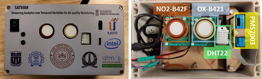
R. Sahu et al.: Robust statistical calibration and characterization of low-cost air quality sensors 39
1.3 Our contributions and the SATVAM initiative 2. Site M. Located within the city of Mumbai (hence
site M) at the Maharashtra Pollution Control Board
The SATVAM (Streaming Analytics over Temporal Vari- (MPCB) within the university campus of IIT Bombay
ables from Air quality Monitoring) initiative has been devel- (19.13◦ N, 72.91◦ E; 50 m a.m.s.l.).
oping low-cost air quality (LCAQ) sensor networks based on
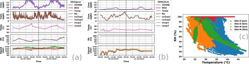
Figure 2 presents a snapshot of raw parameter values pre-
highly portable IoT software platforms. These LCAQ devices
sented by the two sites. We refer readers to the supplemen-
include (see Fig. 3) PM2.5 as well as gas sensors. Details on
tary material for additional details about the two deployment
the IoT software platform and SATVAM node cyber infras-
sites. Due to increasing economic and industrial activities, a
tructure are available in Simmhan et al. (2019). The focus of
progressive worsening of ambient air pollution is witnessed
this paper is to build accurate and robust calibration models
at both sites. We considered these two sites to cover a broader
for the NO2 and O3 gas sensors present in SATVAM devices.
range of pollutant concentrations and weather patterns, so as
Our contributions are summarized below:
to be able to test the reliability of LCAQ networks. It is no-
1. We report the results of a deployment and calibration table that the two chosen sites present different geographical
study involving six sensors deployed at two sites over settings as well as different air pollution levels with site D
two phases with vastly different meteorological, geo- of particular interest in presenting significantly higher mini-
graphical and air quality parameters. mum O3 levels than site M, illustrating the influence of the
geographical variability over the selected region.
2. A unique feature of our deployment is a swap-out exper-
iment wherein three of these sensors were relocated to 2.2 Instrumentation
different sites in the two phases (see Sect. 2 for deploy-
ment details). This allowed us to investigate the efficacy LCAQ sensor design. Each SATVAM LCAQ device contains
of calibration models when applied to weather and air two commodity electrochemical gas sensors (Alphasense
quality conditions vastly different from those present OX-B421 and NO2-B42F) for measuring O3 (ppb) and NO2
during calibration. Such an investigation is missing (ppb) levels, a PM sensor (Plantower PMS7003) for measur-
from previous works which mostly consider only local- ing PM2.5 (µg m−3 ) levels, and a DHT22 sensor for measur-
ized calibration. ing ambient temperature (◦ C) and relative humidity RH (%).
Figure 3 shows the placement of these components. A no-
3. We present an extensive study of parametric and non- table feature of this device is its focus on frugality and use
parametric calibration models and develop a novel local of the low-power Contiki OS platform and 6LoWPAN for
calibration algorithm based on metric learning that of- providing wireless-sensor-network connectivity.
fers stable (across gases, sites and seasons) and accurate Detailed information on assembling these different
calibration. components and the interfacing with an IoT network is
4. We present an analysis of the effect of data preparation described in Simmhan et al. (2019). These sensors form a
techniques, such as volume of data, temporal averag- highly portable IoT software platform to transmit 6LoWPAN
ing and data diversity, on calibration performance. This packets at 5 min intervals containing five time series data
yields several take-home messages that can boost cali- points from individual sensors, namely NO2 , O3 , PM2.5
bration performance. (not considered in this study), temperature and RH. Given
the large number of devices spread across two cities and
seasons in this study, a single border-router edge device was
2 Deployment setup configured at both sites using a Raspberry Pi that acquired
data, integrated them and connected to a cloud facility using
Our deployment employed a network of LCAQ sensors and a Wi-Fi link to the respective campus broadband networks.
reference-grade monitors for measuring NO2 and O3 concen- A Microsoft Azure Standard D4s v3 VM was used to host
trations, deployed at two sites across two phases. the cloud service with four cores, 16 GB RAM and 100 GB
SSD storage running an Ubuntu 16.04.1 LTS OS. The Pi
2.1 Deployment sites edge device was designed to ensure that data acquisition
continues even in the event of cloud VM failure.
SATVAM LCAQ sensor deployment and co-location with
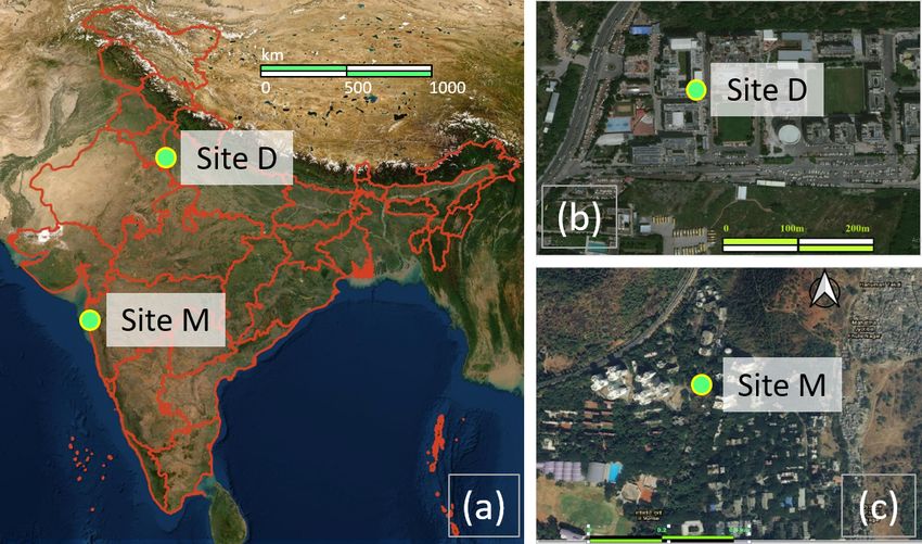
reference monitors was carried out at two sites. Figure 1
Reference monitors. At both the deployment sites, O3 and
presents the geographical locations of these two sites.
NO2 were measured simultaneously with data available at
1. Site D. Located within the Delhi (hence site D) National 1 min intervals for site D deployments (both Jun and Oct)
Capital Region (NCR) of India at the Manav Rachna In- and 15 min intervals for site M deployments. O3 and NO2
ternational Institute of Research and Studies (MRIIRS), values were measured at site D using an ultraviolet photo-
Sector 43, Faridabad (28.45◦ N, 77.28◦ E; 209 m a.m.s.l. metric O3 analyzer (Model 49i O3 analyzer, Thermo Sci-
– above mean sea level). entific™, USA) and a chemiluminescence oxide of nitrogen
https://doi.org/10.5194/amt-14-37-2021 Atmos. Meas. Tech., 14, 37–52, 2021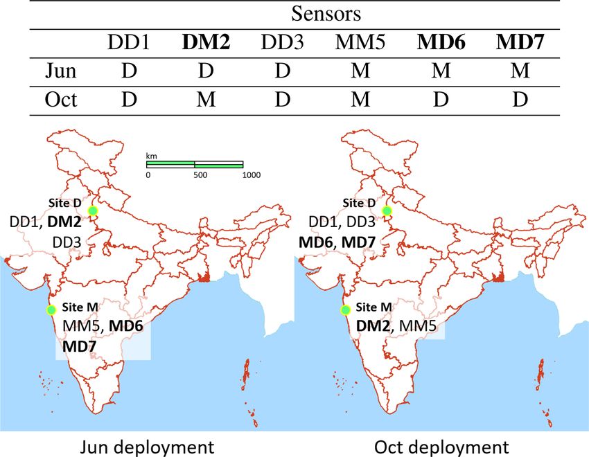
40                         R. Sahu et al.: Robust statistical calibration and characterization of low-cost air quality sensors

Figure 1. A map showing the locations of the deployment sites. Panels (b) and (c) show a local-scale map of the vicinity of the deployment
sites – namely site D at MRIIRS, Delhi NCR (b), and site M at MPCB, Mumbai (c), with the sites themselves pointed out using bright green
dots. Panel (a) shows the location of the sites on a map of India. Credit for map sources: (a) is taken from the NASA Earth Observatory with
the outlines of the Indian states in red taken from QGIS 3.4 Madeira; (b) and (c) are obtained from © Google Maps. The green markers for
the sites in all figures were added separately.

Figure 2. Panels (a, b) present time series for raw parameters measured using the reference monitors (NO2 and O3 concentrations) as well
as those measured using the SATVAM LCAQ sensors (RH, T , no2op1, no2op2, oxop1, oxop2). Panel (a) considers a 48 h period during the
June deployment (1–2 July 2019) at site D with signal measurements taken from the sensor DD1 whereas (b) considers a 48 h period during
the October deployment (20–21 October 2019) at site M with signal measurements taken from the sensor MM5 (see Sect. 2.3 for conventions
used in naming sensors e.g., DD1, MM5). Values for site D are available at 1 min intervals, while those for site M are averaged over 15 min
intervals. Thus, the left plot is more granular than the right plot. Site D experiences higher levels of both NO2 and O3 as compared to site M.
Panel (c) presents a scatterplot showing variations in RH and T at the two sites across the two deployments. The sites offer substantially
diverse weather conditions. Site D exhibits wide variations in RH and T levels during both deployments. Site M exhibits almost uniformly
high RH levels during the October deployment which coincided with the retreating monsoons.

(NOx ) analyzer (Model 42i NOx analyzer, Thermo Scien-                    stalled. These also have a UV photometric analyzer to mea-
tific™, USA), respectively. Regular maintenance and multi-                sure O3 levels and use chemiluminescence to measure NO2
point calibration, zero checks, and zero settings of the in-              concentrations with lowest detectable limits for O3 and NO2
struments were carried out following the method described                 of 0.4 and 0.2 ppb, respectively, and a precision of ± 0.2 and
by Gaur et al. (2014). The lowest detectable limits of ref-               ± 0.1 ppb, respectively. For every deployment, the reference
erence monitors in measuring O3 and NO2 were 0.5 and                      monitors and the AQ sensors were time-synchronized, with
0.40 ppb, respectively, and with a precision of ± 0.25 and                the 1 min interval data averaged across 15 min intervals for
± 0.2 ppb, respectively. Similarly, the deployments at site M             all site M deployments since the site M reference monitors
had Teledyne T200 and T400 reference-grade monitors in-                   gave data at 15 min intervals.

Atmos. Meas. Tech., 14, 37–52, 2021                                                             https://doi.org/10.5194/amt-14-37-2021
R. Sahu et al.: Robust statistical calibration and characterization of low-cost air quality sensors                               41

                                                                      deployment pattern. The name of a sensor is of the form
                                                                      XYn where X (Y) indicates the site at which the sensor
                                                                      was deployed during the June (October) deployment and n
                                                                      denotes its unique numerical identifier. Figure 4 outlines the
                                                                      deployment patterns for the six sensors DD1, DM2, DD3,
                                                                      MM5, MD6 and MD7.

Figure 3. Primary components of the SATVAM LCAQ (low-cost             Swap-out experiment. As Fig. 4 indicates, three sensors were
air-quality) sensor used in our experiments. The SATVAM device        swapped with the other site across the two deployments.
consists of a Plantower PMS7003 PM2.5 sensor, Alphasense OX-          Specifically, for the October deployment, DM2 was shifted
B431 and NO2-B43F electrochemical sensors, and a DHT22 RH             from site D to M and MD6 and MD7 were shifted from site
and temperature sensor. Additional components (not shown here)        M to D.
include instrumentation to enable data collection and transmission.
                                                                      Sensor malfunction. We actually deployed a total of seven
                                                                      sensors in our experiments. The seventh sensor, named DM4,
                                                                      was supposed to be swapped from site D to site M. However,
                                                                      the onboard RH and temperature sensors for this sensor were
                                                                      non-functional for the entire duration of the June deployment
                                                                      and frequently so for the October deployment as well. For
                                                                      this reason, this sensor was excluded from our study alto-
                                                                      gether. To avoid confusion, in the rest of the paper (e.g., the
                                                                      abstract, Fig. 4) we report only six sensors, of which three
                                                                      were a part of the swap-out experiment.

                                                                      3   Data analysis setup

                                                                      All experiments were conducted on a commodity laptop with
                                                                      an Intel Core i7 CPU (2.70 GHz, 8 GB RAM) and running
                                                                      an Ubuntu 18.04.4 LTS operating system. Standard off-the-
                                                                      shelf machine-learning and statistical-analysis packages such
Figure 4. A schematic showing the deployment of the six LCAQ
sensors across site D and site M during the two deployments. The
                                                                      as NumPy, sklearn, SciPy and metric-learn were used to im-
sensors subjected to the swap-out experiment are presented in bold.   plement the calibration algorithms.
Credit for map sources: the outlines of the Indian states in red
are taken from QGIS 3.4 Madeira with other highlights (e.g., for      Raw datasets and features. The six sensors across the June
oceans) and markers being added separately.                           and October deployments gave us a total of 12 datasets.
                                                                      We refer to each dataset by mentioning the sensor name
                                                                      and the deployment. For example, the dataset DM2(Oct)
2.3   Deployment details                                              contains data from the October deployment at site M of the
                                                                      sensor DM2. Each dataset is represented as a collection of
A total of four field co-location deployments, two each at            eight time series for which each timestamp is represented
sites D and M, were evaluated to characterize the calibration         as an 8-tuple (O3 , NO2 , RH, T , no2op1, no2op2, oxop1,
of the low-cost sensors during two seasons of 2019. The two           oxop2) giving us the reference values for O3 and NO2
field deployments at site D were carried out from 27 June–            (in ppb), relative humidity RH (in %) and temperature
6 August 2019 (7 weeks) and 4–27 October 2019 (3 weeks).              T (in ◦ C) values, and voltage readings (in mV) from the
The two field deployments at site M, on the other hand, were          two electrodes present in each of the two gas sensors,
carried out from 22 June–21 August 2019 (10 weeks) and 4–             respectively. These readings represent working (no2op1
27 October 2019 (3 weeks). For the sake of convenience, we            and oxop1) and auxiliary (no2op2 and oxop2) electrode
will refer to both deployments that commenced in the month            potentials for these sensors. We note that RH and T values
of June 2019 (October 2019) as June (October) deployments             in all our experiments were obtained from DHT22 sensors in
even though the dates of both June deployments do not ex-             the LCAQ sensors and not from the reference monitors. This
actly coincide.                                                       was done to ensure that the calibration models, once trained,
   A total of six low-cost SATVAM LCAQ sensors were                   could perform predictions using data available from the
deployed at these two sites. We assign each of these sensors          LCAQ sensor alone and did not rely on data from a reference
a unique numerical identifier and a name that describes its           monitor. For site D, both the LCAQ sensor and the reference

https://doi.org/10.5194/amt-14-37-2021                                                       Atmos. Meas. Tech., 14, 37–52, 2021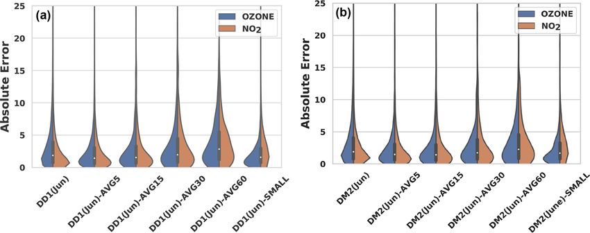
42                        R. Sahu et al.: Robust statistical calibration and characterization of low-cost air quality sensors

Table 1. Samples of the raw data collected from the DM2(June) and MM5(October) datasets. The last column indicates whether data from
that timestamp were used in the analysis or not. Note that DM2(June) data, coming from site D, have samples at 1 min intervals whereas
MM5(October) data, coming from site M, have samples at 15 min intervals. The raw voltage values (no2op1, no2op2, oxop1, oxop2) offered
by the LCAQ sensor are always integer values, as indicated in the DM2(June) data. However, for site M deployments, due to averaging,
the effective-voltage values used in the dataset may be fractional, as indicated in the MM5(October) data. The symbol × indicates missing
values. A bold font indicates invalid values. Times are given in local time.

                                                              DM2(June)
      Timestamp            O3       NO2         T     RH    no2op1     no2op2         oxop1    oxop2   no2diff    oxdiff   Valid?
      29 Jun 04:21      19.82     20.49      32.7    54.6       212          231        242      209     −19         33       Yes
      30 Jun 08:02     46.363    −0.359      36.8    39.6       184          221        234      201     −37         33       No
      01 Jul 04:02      24.38     14.73      32.5    69.7        ×            ×          ×        ×       ×          ×        No
      08 Jul 07:51     −0.035    17.147      31.5    97.8       209          238        231      216     −29         15       No
                                                               MM5(Oct)
      Timestamp            O3       NO2         T     RH    no2op1     no2op2         oxop1    oxop2   no2diff    oxdiff   Valid?
      19 Oct 05:45          ×         ×        ×       ×     160.46     188.31       158.31   172.38   −27.85    −14.07       No
      19 Oct 07:15        5.55     11.52    41.47    99.9     170.4      197.2        167.6   181.93    −26.8    −14.33       Yes
      20 Oct 10:45          ×         ×     28.52    99.9     121.8      154.0        119.3    135.3    −32.2     −16.0       No
      22 Oct 18:30        8.33     10.91    27.87    99.9     143.2      172.3        146.2   155.47    −29.1     −9.27       Yes

monitor data were available at 1 min intervals. However for            both sites, more data are available for the June deployment
site M, since reference monitor data were only available               (that lasted longer) than the October deployment.
at 15 min intervals, LCAQ sensor data were averaged over
15 min intervals.                                                      3.1     Data augmentation and derived dataset creation

Data cleanup. Timestamps from the LCAQ sensors were                    For each of the 12 datasets, apart from the six data features
aligned to those from the reference monitors. For several              provided by the LCAQ sensors, we included two augmented
timestamps, we found that either the sensor or reference               features, calculated as follows: no2diff = no2op1 − no2op2,
monitors presented at least one missing or spurious value (see         and oxdiff = oxop1−oxop2. We found that having these aug-
Table 1 for examples). Spurious values included the follow-            mented features, although they are simple linear combina-
ing cases: (a) a reference value for O3 or NO2 of > 200 ppb            tions of raw features, offered our calibration models a pre-
or < 0 ppb (the reference monitors sometimes offered nega-             dictive advantage. The augmented datasets created this way
tive readings when powering up and under anomalous oper-               represented each timestamp as a vector of eight feature val-
ating conditions, e.g., condensation at the inlet), (b) a sensor       ues (RH, T , no2op1, no2op2, oxop1, oxop2, no2diff, oxdiff),
temperature reading of > 50 ◦ C or < 1 ◦ C, (c) a sensor RH            apart from the reference values of O3 and NO2 .
level of > 100 % or < 1 %, and (d) a sensor voltage read-
ing (any of no2op1, no2op2, oxop1, oxop2) of > 400 mV or               3.1.1       Train–test splits
< 1 mV. These errors are possibly due to electronic noise in
the devices. All timestamps with even one spurious or miss-            Each of the 12 datasets was split in a 70 : 30 ratio to obtain a
ing value were considered invalid and removed. Across all 12           train–test split. For each dataset, 10 such splits were indepen-
datasets, an average of 52 % of the timestamps were removed            dently generated. All calibration algorithms were given the
as a result. However, since site D (site M) offered timestamps         same train–test splits. For algorithms that required hyperpa-
at 1 min (15 min) intervals i.e., 60 (4) timestamps every hour,        rameter tuning, a randomly chosen set of 30 % of the training
at least one valid timestamp (frequently several) was still            data points in each split was used as a held-out validation set.
found every hour in most cases. Thus, the valid timestamps             All features were normalized to improve the conditioning of
could still accurately track diurnal changes in AQ parame-             the calibration problems. This was done by calculating the
ters. The datasets from June (October) deployments at site D           mean and standard deviation for each of the eight features on
offered an average of 33 753 (9548) valid timestamps. The              the training portion of a split and then mean centering and
datasets from June (October) deployments in site M offered             dividing by the standard deviation all timestamps in both the
an average of 2462 (1062) valid timestamps. As expected,               training and the testing portion of that split. An exception
site D which had data at 1 min intervals offered more times-           was made for the Alphasense calibration models, which re-
tamps than site M which had data at 15 min intervals. For              quired raw voltage values. However, reference values were
                                                                       not normalized.

Atmos. Meas. Tech., 14, 37–52, 2021                                                           https://doi.org/10.5194/amt-14-37-2021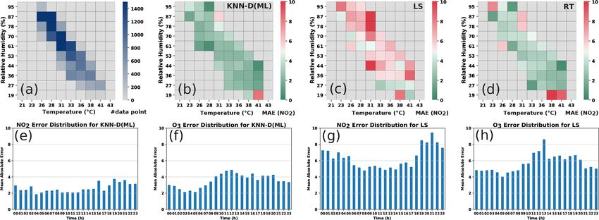
R. Sahu et al.: Robust statistical calibration and characterization of low-cost air quality sensors                             43

3.2   Derived datasets                                             3.2.1   Performance evaluation

In order to study the effect of data frequency (how frequently     The performance of calibration algorithms was assessed
do we record data, e.g., 1 min, 15 min?), data volume (total       using standard error metrics and statistical hypothesis testing.
number of timestamps used for training) and data diversity
(data collected across seasons or sites) on the calibration per-   Error metrics. Calibration performance was measured using
formance, we created several derived datasets as well. All         four popular metrics: mean absolute error (MAE), mean
these datasets contained the augmented features.                   absolute percentage error (MAPE), root mean squared error
                                                                   (RMSE), and the coefficient of determination (R 2 ) (please
 1. Temporally averaged datasets. We took the two datasets         see the supplementary material for detailed expressions of
    DD1(Jun) and DM2(Jun) and created four datasets out            these metrics).
    of each of them by averaging the sensor and reference
    monitor values at 5, 15, 30 and 60 min intervals. These        Statistical hypothesis tests. In order to compare the perfor-
    datasets were named by affixing the averaging inter-           mance of different calibration algorithms on a given dataset
    val size to the dataset name. For example, DD1(Jun)-           (to find out the best-performing algorithm) or to compare the
    AVG5 was created out of DD1(Jun) by performing                 performance of the same algorithm on different datasets (to
    5 min averaging and DM2(Jun)-AVG30 was created out             find out the effect of data characteristics on calibration per-
    of DM2(Jun) using 30 min averaging.                            formance), we performed paired and unpaired two-sample
                                                                   tests, respectively. Our null hypothesis in all such tests pro-
 2. Sub-sampled datasets. To study the effect of having            posed that the absolute errors offered in the two cases con-
    fewer training data on calibration performance, we             sidered are distributed identically. The test was applied, and
    created sub-sampled versions of both these datasets            if the null hypothesis was rejected with sufficient confidence
    by sampling a random set of 2500 timestamps from               (an α value of 0.05 was used as the standard to reject the
    the training portion of the DD1(June) and DM2(June)            null hypotheses), then a winner was simultaneously identi-
    datasets to get the datasets named DD1(June)-SMALL             fied. Although Student’s t test is more popular, it assumes
    and DM2(June)-SMALL.                                           that the underlying distributions are normal, and an appli-
                                                                   cation of the Shapiro–Wilk test (Shapiro and Wilk, 1965)
 3. Aggregated datasets. Next, we created new datasets             to our absolute error values rejected the normal hypothesis
    by pooling data for a sensor across the two deploy-            with high confidence. Thus, we chose the non-parametric
    ments. This was done to the data from the sensors              Wilcoxon signed-rank test (Wilcoxon, 1945) when compar-
    DD1, MM5, DM2 and MD6. For example, if we con-                 ing two algorithms on the same dataset and its unpaired vari-
    sider the sensor DD1, then the datasets DD1(June)              ant, the Mann–Whitney U test (Mann and Whitney, 1947)
    and DD1(October) were combined to create the dataset           for comparing the same algorithm on two different datasets.
    DD1(June–October).                                             These tests do not make any assumption about the underlying
                                                                   distribution of the errors and are well-suited for our data.
Investigating impact of diversity in data. The aggregated
datasets are meant to help us study how calibration al-
gorithms perform under seasonally and spatially diverse
data. For example, the datasets DD1(June–October) and              4   Baseline and proposed calibration models
MM5(June–October) include data that are seasonally diverse
but not spatially diverse (since these two sensors were lo-        Our study considered a large number of parametric and non-
cated at the same site for both deployments). On the other         parametric calibration techniques as baseline algorithms. Ta-
hand, the datasets DM2(June–October) and MD6(June–                 ble 2 provides a glossary of all the algorithms including
October) include data that are diverse both seasonally and         their acronyms and brief descriptions. Detailed descriptions
spatially (since these two sensors were a part of the swap-        of all these algorithms are provided in the supplementary
out experiment). At this point, it is natural to wonder about      material. Among parametric algorithms, we considered the
studying the effect of spatial diversity alone (without sea-       Alphasense models (AS1–AS4) supplied by the manufac-
sonal effects). This can be done by aggregating data from          turers of the gas sensors and linear models based on least
two distinct sensors since no sensor was located at both sites     squares (LS and LS(MIN)) and sparse recovery (LASSO).
during a deployment. However, this turns out to be challeng-       Among non-parametric algorithms, we considered the re-
ing since the onboard sensors in the LCAQ devices, e.g., RH        gression tree (RT) method, kernel-ridge regression (KRR),
and T sensors, do not present good agreement across devices,       the Nystroem method for accelerating KRR, the Nadaraya–
and some form of cross-device calibration is needed. This is       Watson (NW) estimator and various local algorithms based
an encouraging direction for future work but not considered        on the k nearest-neighbors principle (KNN, KNN-D). In this
in this study.                                                     section we give a self-contained description of our proposed

https://doi.org/10.5194/amt-14-37-2021                                                    Atmos. Meas. Tech., 14, 37–52, 2021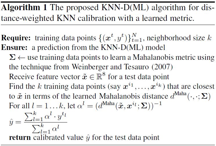
44                        R. Sahu et al.: Robust statistical calibration and characterization of low-cost air quality sensors

algorithms KNN(ML) and KNN-D(ML).                                    T , seem to have a significant influence on calibration perfor-
                                                                     mance. Thus, it is unclear how much emphasis RH and T
Notation. For every timestamp t, the vector x t ∈ R8 denotes         should receive, as compared to other features such as volt-
the 8-dimensional vector of signals recorded by the LCAQ             age values, e.g., oxop1, while calculating distances between
sensors for that timestamp (namely, RH, T , no2op1, no2op2,          two points. The technique of metric learning (Weinberger
oxop1, oxop2, no2diff, oxdiff), while the vector y t ∈ R2 will       and Saul, 2009) offers a solution in this respect by learning a
denote the 2-tuple of the reference values of O3 and NO2             customized Mahalanobis metric that can be used instead of
for that time step. However, this notation is unnecessarily          the generic Euclidean metric. A Mahalanobis metric is char-
cumbersome since we will build separate calibration mod-             acterized by a positive semi-definite matrix 6 ∈ R8×8 and
els for O3 and NO2 . Thus, to simplify the notation, we will         calculates the distance between any two points as follows:
instead use y t ∈ R to denote the reference value of the gas
being considered (either O3 or NO2 ). The goal of calibration                                   p
                                                                     d Maha (x 1 , x 2 ; 6) =       (x 1 − x 2 )> 6(x 1 − x 2 ).
will then be to learn a real-valued function f : R8 → R such
that f (x t ) ≈ y t for all timestamps t (the exact error being
measured using metrics such as MAE or MAPE). Thus, two               Note that the Mahalanobis metric recovers the Euclidean
functions will be learned, say fNO2 and fO3 , to calibrate for       metric if we choose 6 = I8 , i.e., the identity matrix. Now,
NO2 and O3 concentrations, respectively. Since our calibra-          whereas metric learning for KNN is popular for classifica-
tion algorithms use statistical estimation or machine learning       tion problems, it is uncommon for calibration and regres-
algorithms, we will let N (n) denote the number of training          sion problems. This is due to regression problems lack-
(testing) points for a given dataset and split thereof. Thus,        ing a small number of “classes”. To overcome this prob-
{(x t , y t )}N                                                      lem, we note that other non-parametric calibration algo-
              t=1 will denote the training set for a given dataset
and split with x t ∈ R8 and y t ∈ R.                                 rithms such as NW and KRR also utilize a metric indirectly
                                                                     (please see the supplementary material) and there exist tech-
4.1   Proposed method – distance-weighed KNN with a                  niques to learn a Mahalanobis metric to be used along with
      learned metric                                                 these algorithms (Weinberger and Tesauro, 2007). This al-
                                                                     lows us to adopt a two-stage algorithm that first learns a
Our proposed algorithm is a local, non-parametric algorithm          Mahalanobis metric well-suited for use with the NW algo-
that uses a learned metric. Below we describe the design of          rithm and then uses it to perform KNN-style calibration. Al-
this method and reasons behind these design choices.                 gorithm 1 describes the resulting KNN-D(ML) algorithm.

Non-parametric estimators for calibration. The simplest
example of a non-parametric estimator is the KNN (k
nearest-neighbors) algorithm that predicts, for a test point,
the average reference value in the k most similar training
points also known as “neighbors”. Other examples of
non-parametric algorithms include kernel ridge regression
(KRR) and the Nadaraya–Watson (NW) estimator (please
see the supplementary material for details). Non-parametric
estimators are well-studied and known to be asymptotically
universal which guarantees their ability to accurately model
complex patterns which motivated our choice. These models
can also be brittle (Hagan et al., 2019) when used in unseen
operating conditions, but Sect. 5.2 shows that our proposed
algorithm performs comparably to parametric algorithms
when generalizing to unseen conditions but offers many
more improvements when given additional data.                        5   Results and discussion

Metric learning for KNN calibration. As mentioned above,             The goals of using low-cost AQ monitoring sensors vary
the KNN algorithm uses neighboring points to perform pre-            widely. This section critically assesses a wide variety of cal-
diction. A notion of distance, specifically a metric, is required    ibration models. First we look at the performance of the al-
to identify neighbors. The default and most common choice            gorithms on individual datasets, i.e., when looking at data
for a metric is the Euclidean distance which gives equal im-         within a site and within a season. Next, we look at derived
portance to all eight dimensions when calculating distances          datasets (see Sect. 3.2) which consider the effect of data vol-
between two points, say x 1 , x 2 ∈ R8 . However, our experi-        ume, data averaging and data diversity on calibration perfor-
ments in Sect. 5 will show that certain features, e.g., RH and       mance.

Atmos. Meas. Tech., 14, 37–52, 2021                                                         https://doi.org/10.5194/amt-14-37-2021
R. Sahu et al.: Robust statistical calibration and characterization of low-cost air quality sensors 45
Table 2. Glossary of baseline and proposed calibration algorithms used in our study with their acronyms and brief descriptions. The
KNN(ML) and KNN-D(ML) algorithms are proposed in this paper. Please see the Supplement for details.
Parametric algorithms Non-parametric algorithms Non-parametric KNN-style algorithms
AS1, AS2 Alphasense models RT Regression tree KNN k nearest neighbors
AS3, AS4 (From gas sensor manufacturer) KRR Kernel ridge regression KNN-D Distance-weighted KNN
LS Least-squares regression NYS Nystroem method KNN(ML)∗ KNN (learned metric)
LS(MIN) LS with reduced features NW(ML) Nadaraya–Watson (learned metric) KNN-D(ML)∗ KNN-D (learned metric)
LASSO Sparse regression
∗ Proposed in this paper.
Table 3. Results of the pairwise Wilcoxon signed-rank tests across all model types. We refer the reader to Sect. 5.1.1 for a discussion on
how to interpret this table. KNN-D(ML) beats every other algorithm comprehensively and is scarcely ever beaten (with the exception of
NW(ML), which KNN-D(ML) still beats 58 % of the time for NO2 and 62 % of the time for O3 ). The overall ranking of the algorithms is
indicated to be KNN-D(ML) > NW(ML) > KRR > RT > LS.
NO2 O3
LS RT KRR NW(ML) KNN-D(ML) LS RT KRR NW(ML) KNN-D(ML)
LS 0 0 0 0 0 0 0.01 0 0 0
RT 0.97 0 0.38 0.16 0 0.83 0 0.22 0 0
KRR 1 0.4 0 0 0 1 0.63 0 0.01 0
NW(ML) 1 0.75 1 0 0.07 1 0.97 0.96 0 0.02
KNN-D(ML) 1 1 1 0.58 0 1 1 0.97 0.62 0
5.1 Effect of model on calibration performance gets 0) or else the null hypothesis is not refuted (in which
case both get 0). The average of these scores is then shown.
We compare the performance of calibration algorithms in- For example, in Table 3, row 3–column 7 (excluding column
troduced in Sect. 4. Given the vast number of algorithms, and row headers) records a value of 0.63 implying that in
we executed a tournament where algorithms were divided 63 % of these tests, KRR won over RT in the case of O3 cal-
into small families, decided the winner within each family ibration, whereas row 2–column 8 records a value of 0.22,
and then compared winners across families. The detailed per- implying that in 22 % of the tests, RT won over KRR. On
family comparisons are available in the supplementary mate- balance (1 − 0.63 − 0.22 = 0.15) i.e., 15 % of the tests, nei-
rial and summarized here. The Wilcoxon paired two-sample ther algorithm could be declared a winner.
test (see Sect. 3.2.1) was used to compare two calibration al-
gorithms on the same dataset. However, for visual inspection, 5.1.2 Intra-family comparison of calibration models
we also provide violin plots of the absolute errors offered by
the algorithms. We refer the reader to the supplementary ma-
We divided the calibration algorithms (see Table 2 for
terial for pointers on how to interpret violin plots.
a glossary) into four families: (1) the Alphasense fam-
ily (AS1, AS2, AS3, AS4), (2) linear parametric models
5.1.1 Interpreting the two-sample tests
(LS, LS(MIN) and LASSO), (3) kernel regression models
We refer the reader to Table 2 for a glossary of algorithm (KRR, NYS), and (4) KNN-style algorithms (KNN, KNN-
names and abbreviations. As mentioned earlier, we used the D, NW(ML), KNN(ML), KNN-D(ML)). We included the
paired Wilcoxon signed-rank test to compare two algorithms Nadaraya–Watson (NW) algorithm in the fourth family since
on the same dataset. Given that there are 12 datasets and 10 it was used along with metric learning, as well as because as
splits for each dataset, for ease of comprehension, we pro- explained in the supplementary material, the NW algorithm
vide globally averaged statistics of wins scored by an algo- behaves like a “smoothed” version of the KNN algorithm.
rithm over another. For example, say we wish to compare RT The winners within these families are described below.
and KRR as done in Table 3, we perform the test for each
individual dataset and split. For each test, we get a win for 1. Alphasense. All four Alphasense algorithms exhibit ex-
RT (in which case RT gets a +1 score and KRR gets 0) or tremely poor performance across all metrics on all
a win for KRR (in which case KRR gets a +1 score and RT datasets, offering extremely high MAE and low R 2 val-
https://doi.org/10.5194/amt-14-37-2021 Atmos. Meas. Tech., 14, 37–52, 202146 R. Sahu et al.: Robust statistical calibration and characterization of low-cost air quality sensors
ues. This is corroborated by previous studies (Lewis and
indicate the best-performing algorithm in terms of mean statistics.
Table 4. A comparison of algorithms across families on the DD1 and MM5 datasets across seasons with respect to the R 2 metric. All values are averaged across 10 splits. Bold values
KNN-D(ML)
NW(ML)
KRR
RT
LS
Edwards, 2016; Jiao et al., 2016; Simmhan et al., 2019).
2. Linear parametric. Among the linear parametric algo-
rithms, LS was found to offer the best performance.
3. Kernel regression. The Nystroem method (NYS) was
0.923 ± 0.003
0.895 ± 0.004
0.885 ± 0.005
0.852 ± 0.005
0.843 ± 0.006 confirmed to be an accurate but accelerated approxi-
mation for KRR with the acceleration being higher for
June larger datasets.
DD1
4. KNN and metric-learning models. Among the KNN
family of algorithms, KNN-D(ML), i.e., distance-
0.988 ± 0.001
0.987 ± 0.002
0.971 ± 0.003
0.969 ± 0.002
0.99 ± 0.001
weighted KNN with a learned metric, was found to offer
O3
October
the best accuracies across all datasets and splits.
5.1.3 Global comparison of comparison models
0.744 ± 0.043
0.719 ± 0.037
0.488 ± 0.071
0.334 ± 0.035
We took the best algorithms from all the families (except Al-
0.74 ± 0.038
phasense models that gave extremely poor performance) and
regression trees (RT) and performed a head-to-head compar-
June
ison to assess the winner. The two-sample tests (Table 3) as
MM5
well as violin plots (Fig. 5) indicate that the KNN-D(ML) al-
0.943 ± 0.025
0.943 ± 0.026
gorithm continues to emerge as the overall winner. Table 4
0.393 ± 0.224
0.846 ± 0.019
0.935 ± 0.02
additionally establishes that KNN-D(ML) can be up to 4–
October
20 percentage points better than classical non-parametric al-
gorithms such as KRR in terms of the R 2 coefficient. The
improvement is much more prominent for NO2 calibration
which seems to be more challenging as compared to O3
calibration. Figure 6 presents cases where the KNN-D(ML)
0.819 ± 0.015
0.717 ± 0.017
0.608 ± 0.019
0.674 ± 0.015
0.341 ± 0.013
models offer excellent agreement with the reference moni-
tors across significant spans of time.
June
Analyzing high-error patterns. Having analyzed the cali-
DD1
bration performance of various algorithms including KNN-
0.977 ± 0.002
0.957 ± 0.003
0.913 ± 0.014
0.623 ± 0.005
0.97 ± 0.003
D(ML), it is interesting to note under what conditions these
algorithms incur high error. Non-parametric algorithms such
October
as RT and KNN-D(ML) are expected to do well in the pres-
ence of good quantities of diverse data. Figure 7 confirms
NO2
this by classifying timestamps into various bins according to
0.771 ± 0.026
0.759 ± 0.022
0.728 ± 0.034
0.487 ± 0.064
0.375 ± 0.049
weather conditions. KNN-D(ML) and RT give high average
error mostly in those bins where there were fewer training
points. Figure 7 also confirms a positive correlation between
June
high concentrations and higher error although this effect is
MM5
more pronounced for LS than for KNN-D(ML).
0.751 ± 0.043
0.751 ± 0.039
0.673 ± 0.059
0.358 ± 0.087
0.321 ± 0.026
5.2 Effect of data preparation on calibration
performance
October
We critically assessed the robustness of these calibration
models and identified the effect of other factors, such as tem-
poral averaging of raw data, total number of data available
for training and diversity in training data. We note that some
of these studies were made possible only because the swap-
out experiment enabled us to have access to sensors that did
not change their deployment sites, as well as to those that did
change their deployment site.
Atmos. Meas. Tech., 14, 37–52, 2021 https://doi.org/10.5194/amt-14-37-2021R. Sahu et al.: Robust statistical calibration and characterization of low-cost air quality sensors 47
Figure 5. The violin plots on the left (a) show the distribution of absolute errors incurred by various models on the DD1(October)
(MM5(June)) datasets. KNN-D(ML) offers visibly superior performance as compared to other algorithms such as LS and RT.
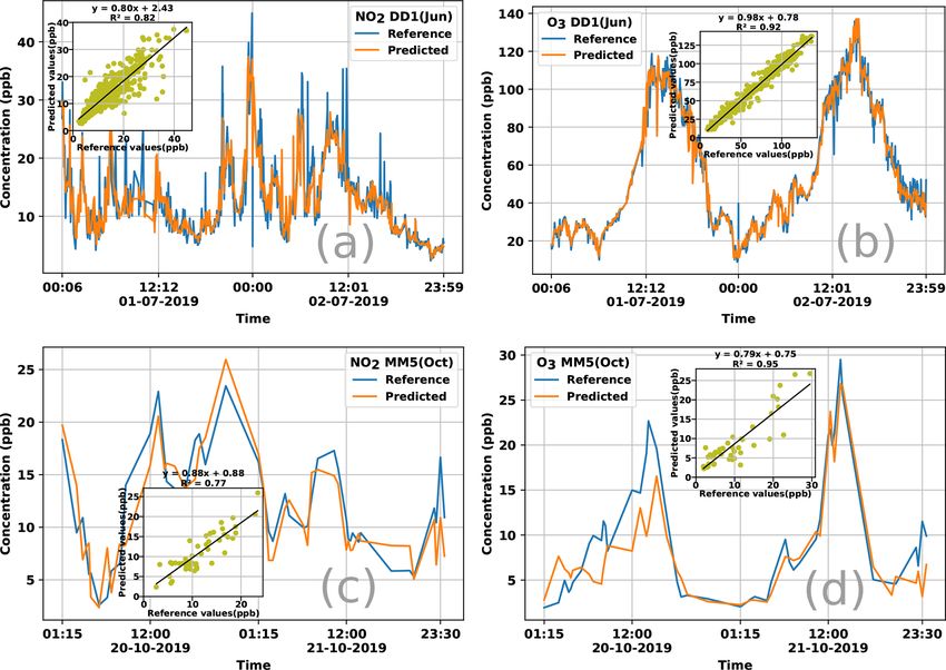
Figure 6. Time series plotting reference values and those predicted by the KNN-D(ML) algorithm for NO2 and O3 concentration for 48 h
durations using data from the DD1 and MM5 sensors. The legend of each plot notes the gas for which calibration is being reported and
the deployment season, as well as the sensor from which data were used to perform the calibration. Each plot also contains a scatterplot as
an inset showing the correlation between the reference and predicted values of the concentrations. For both deployments and both gases,
KNN-D(ML) can be seen to offer excellent calibration and agreement with the FRM-grade monitor.
5.2.1 Some observations on original datasets affecting calibration performance negatively, as well as that
O3 calibration might be less sensitive to these factors than
The performance of KNN-D(ML) on the original datasets NO2 calibration.
itself gives us indications of how various data preparation
methods can affect calibration performance. Table 4 shows 5.2.2 Effect of temporal data averaging
us that in most cases, the calibration performance is better
(with higher R 2 ) for O3 than for NO2 . This is another in- Recall that data from sensors deployed at site M had to be
dication that NO2 calibration is more challenging than O3 averaged over 15 min intervals to align them with the refer-
calibration. Moreover, for both gases and in both seasons, ence monitor timestamps. To see what effect such averaging
we see site D offering a better performance than site M. This has on calibration performance, we use the temporally av-
difference is more prominent for NO2 than for O3 . This in- eraged datasets (see Sect. 3.1). Figure 8 presents the results
dicates that paucity of data and temporal averaging may be of applying the KNN-D(ML) algorithm on data that are not
https://doi.org/10.5194/amt-14-37-2021 Atmos. Meas. Tech., 14, 37–52, 202148 R. Sahu et al.: Robust statistical calibration and characterization of low-cost air quality sensors
Figure 7. Analyzing error distributions of LS, KNN-D(ML) and RT. Panel (a) shows the number of training data points in various weather
condition bins. Panels (b, c, d) show the MAE for NO2 calibration offered by the algorithms in those same bins. Non-parametric algorithms
such as KNN-D(ML) and RT offer poor performance (high MAE) mostly in bins that had fewer training data. No such pattern is observable
for LS. Panels (e, f, g, h) show the diurnal variation in MAE for KNN-D(ML) and LS at various times of day. O3 errors exhibit a diurnal trend
of being higher (more so for LS than for KNN-D(ML)) during daylight hours when O3 levels are high. No such trend is visible for NO2 .
Figure 8. Effect of temporal data averaging and lack of data on the calibration performance of the KNN-D(ML) algorithm on temporally
averaged and sub-sampled versions of the DD1(June) and DM2(June) datasets. Notice the visible deterioration in the performance of the al-
gorithm when aggressive temporal averaging, e.g., across 30 min windows, is performed. NO2 calibration performance seems to be impacted
more adversely than O3 calibration by lack of enough training data or aggressive averaging.
averaged at all (i.e., 1 min interval timestamps), as well as pacted more adversely than O3 calibration by aggressive av-
data that are averaged at 5, 15, 30 and 60 min intervals. The eraging.
performance for 30 and 60 min averaged datasets is visibly
inferior than for the non-averaged dataset as indicated by the
violin plots. This leads us to conclude that excessive aver- 5.2.3 Effect of data paucity
aging can erode the diversity of data and hamper effective
calibration. To distinguish among the other temporally aver-
aged datasets for which visual inspection is not satisfactory, Since temporal averaging decreases the number of data as a
we also performed the unpaired Mann–Whitney U test, the side-effect, in order to tease these two effects (of the tem-
results for which are shown in Table 5. The results are strik- poral averaging and of the paucity of data) apart, we also
ing in that they reveal that moderate averaging, for example considered the sub-sampled versions of these datasets (see
at 5 min intervals, seems to benefit calibration performance. Sect. 3.1). Figure 8 also shows that reducing the number
However, this benefit is quickly lost if the averaging window of training data has an appreciable negative impact on cal-
is increased much further, at which point performance almost ibration performance. NO2 calibration performance seems to
always suffers. NO2 calibration performance seems to be im- be impacted more adversely than O3 calibration by lack of
enough training data.
Atmos. Meas. Tech., 14, 37–52, 2021 https://doi.org/10.5194/amt-14-37-2021R. Sahu et al.: Robust statistical calibration and characterization of low-cost air quality sensors 49
Table 5. Results of the pairwise Mann–Whitney U tests on the performance of KNN-D(ML) across temporally averaged versions of the DD1
dataset. We refer the reader to Sect. 5.1.1 for a discussion on how to interpret this table. The dataset names are abbreviated, e.g., DD1(June)-
AVG5 is referred to as simply AVG5. Results are reported over a single split. AVG5 wins over any other level of averaging and clarifies that
mild temporal averaging (e.g., over 5 min windows) boosts calibration performance, whereas aggressive averaging, e.g., 60 min averaging in
AVG60, degrades performance.
O3 NO2
DD1(June) AVG5 AVG15 AVG30 AVG60 DD1(June) AVG5 AVG15 AVG30 AVG60
DD1(June) 0 0 0 0 0 DD1(June) 0 0 0 1 1
AVG5 1 0 1 1 1 AVG5 1 0 1 1 1
AVG15 1 0 0 1 1 AVG15 0 0 0 1 1
AVG30 1 0 0 0 1 AVG30 0 0 0 0 1
AVG60 0 0 0 0 0 AVG60 0 0 0 0 0
Table 6. A demonstration of the impact of data diversity and data volume on calibration performance. All values are averaged across 10
splits. The results for LS diverged for some of the datasets for a few splits, and those splits were removed while averaging to give LS an
added advantage. Bold values indicate the better-performing algorithm. The first two rows present the performance of the KNN-D(ML) and
LS calibration models when tested on data for a different season (deployment) but in the same site. This was done for the DD1 and MM5
sensors that did not participate in the swap-out experiment. The next two rows present the same but for sensors DM2 and MD6 that did
participate in the swap-out experiment, and thus, their performance is being tested for not only a different season but also a different site.
The next four rows present the dramatic improvement in calibration performance once datasets are aggregated for these four sensors. NO2
calibration is affected worse by these variations (average R 2 in first four rows being −3.69) than O3 calibration (average R 2 in first four
rows being −0.97).
KNN-D(ML) LS
O3 NO2 O3 NO2
Train → test MAE R2 MAE R2 MAE R2 MAE R2
DD1(Jun) → (Oct) 21.82 0.19 21.86 −0.64 12.88 0.73 12.73 0.22
MM5(Oct) → (Jun) 8.33 −3.75 15.79 −12.28 10.39 −4.83 17.06 −21.67
DM2(Jun) → (Oct) 13.04 0.41 9.05 −0.99 9.36 0.68 5.95 0.1
MD6(Jun) → (Oct) 16.71 −0.72 30.9 −0.85 21.12 −1.29 25.67 −0.23
DD1(Jun–Oct) 3.3 0.956 2.6 0.924 11.7 0.29 13.0 0.38
MM5(Jun–Oct) 2.5 0.902 1.8 0.814 4.28 0.32 5.51 0.67
DM2(Jun–Oct) 3.7 0.916 2.8 0.800 6.13 0.79 6.72 0.26
MD6(Jun–Oct) 1.9 0.989 1.8 0.975 7.01 0.71 6.36 0.91
5.2.4 The swap-out experiment – effect of data faced with unseen RH and T ranges. To verify that this is
diversity indeed the case, we ran the KNN-D(ML) algorithm on the
aggregated datasets (see Sect. 3.1) which combine training
Table 6 describes an experiment wherein we took the KNN- sets from the two deployments of these sensors. Table 6 con-
D(ML) model trained on one dataset and used it to make pre- firms that once trained on these more diverse datasets, the
dictions on another dataset. To avoid bringing in too many algorithms resume offering good calibration performance on
variables such as cross-device calibration (see Sect. 3.2), this the entire (broadened) range of RH and T values. However,
was done only in cases where both datasets belonged to the KNN-D(ML) is more superior at exploiting the additional di-
same sensor but for different deployments. Without excep- versity in data than LS. We note that parametric models are
tion, such “transfers” led to a drop in performance. We con- expected to generalize better than non-parametric models for
firmed that this was true for not just non-parametric meth- unseen conditions, and indeed we observe this in some cases
ods such as KNN-D(ML) but also parametric models like in Table 6 where, for DD1 and DM2 datasets, LS generalized
LS. This is to be expected since the sites D and M expe- better than KNN-D(ML). However, we also observe some
rience largely non-overlapping ranges of RH and T across cases such as MM5 and MD6 where KNN-D(ML) general-
the two deployments (see Fig. 2c for a plot of RH and T izes comparably to or better than LS.
values experienced at both sites in both deployments). Thus,
it is not surprising that the models performed poorly when
https://doi.org/10.5194/amt-14-37-2021 Atmos. Meas. Tech., 14, 37–52, 202150 R. Sahu et al.: Robust statistical calibration and characterization of low-cost air quality sensors
6 Conclusions and future work Supplement. The supplement related to this article is available on-
line at: https://doi.org/10.5194/amt-14-37-2021-supplement.
In this study we presented results of field deployments of
LCAQ sensors across two seasons and two sites having di-
verse geographical, meteorological and air pollution param- Author contributions. RaS and BM performed measurements. RaS,
eters. A unique feature of our deployment was the swap-out AN, KKD, HU and PK processed and analyzed the data. RaS, AN
experiment wherein three of the six sensors were transported and PK wrote the paper. AN and PK developed the KNN-D(ML)
across sites in the two deployments. To perform highly ac- calibration algorithm described in Sect. 4 and conducted the data
curate calibration of these sensors, we experimented with a analysis experiments reported in Sect. 5. SM, SN and YS designed
and set up the IoT cyber-infrastructure required for data acquisition
wide variety of standard algorithms but found a novel method
from the edge to the cloud. BM, RoS and RZ designed the SATVAM
based on metric learning to offer the strongest results. A few LCAQ device and did hardware assembly and fabrication. VMM
key takeaways from our statistical analyses are as follows: provided reference-grade data from site M used in this paper. SNT
1. Incorporating ambient RH and T , as well as the aug- supervised the project, designed and conceptualized the research,
mented features oxdiff and noxdiff (see Sect. 3), into the provided resources, acquired funding, and helped in writing and re-
vising the paper.
calibration model improves calibration performance.
2. Non-parametric methods such as KNN offer the best
performance but stand to gain significantly through Competing interests. Author Ronak Sutaria is the CEO of Respirer
the use of metric-learning techniques, which automat- Living Sciences Pvt. Ltd. which builds and deploys low-cost-
ically learn the relative importance of each feature, as sensor-based air quality monitors with the trade name “Atmos – Re-
well as hyper-local variations such as distance-weighted altime Air Quality”. Ronak Sutaria’s involvement was primarily in
the development of the air quality sensor monitors and the big-data-
KNN. The significant improvements offered by non-
enabled application programming interfaces used to access the tem-
parametric methods indicate that these calibration tasks poral data but not in the data analysis. Author Brijesh Mishra, sub-
operate in high-variability conditions where local meth- sequent to the work presented in this paper, has joined the Respirer
ods offer the best chance of capturing subtle trends. Living Sciences team. The authors declare that they have no other
competing interests.
3. Performing smoothing over raw time series data ob-
tained from the sensors may help improve calibration
performance but only if done over short windows. Very
Acknowledgements. This research has been supported under the
aggressive smoothing done over long windows is detri- Research Initiative for Real Time River Water and Air Quality Mon-
mental to performance. itoring program funded by the Department of Science and Technol-
ogy, government of India, and Intel® and administered by the Indo-
4. Calibration models are data-hungry as well as diversity-
United States Science and Technology Forum (IUSSTF).
hungry. This is especially true of local methods, for in-
stance KNN variants. Using these techniques limits the
number of data or diversity of data in terms of RH, T
Financial support. This research has been supported by the Indo-
or concentration levels, which may result in calibration United States Science and Technology Forum (IUSSTF) (grant no.
models that generalize poorly. IUSSTF/WAQM-Air Quality Project-IIT Kanpur/2017).
5. Although all calibration models see a decline in perfor-
mance when tested in unseen operating conditions, cal-
Review statement. This paper was edited by Pierre Herckes and re-
ibration models for O3 seem to be less sensitive than
viewed by three anonymous referees.
those for NO2 calibration.
Our results offer encouraging options for using LCAQ
sensors to complement CAAQMSs in creating dense and
portable monitoring networks. Avenues for future work in-
clude the study of long-term stability of electrochemical sen- References
sors, characterizing drift or deterioration patterns in these
sensors and correcting for the same, and the rapid calibra- Akasiadis, C., Pitsilis, V., and Spyropoulos, C. D.: A Multi-Protocol
tion of these sensors that requires minimal co-location with IoT Platform Based on Open-Source Frameworks, Sensors, 19,
a reference monitor. 4217, 2019.
Apte, J. S., Messier, K. P., Gani, S., Brauer, M., Kirchstetter, T. W.,
Lunden, M. M., Marshall, J. D., Portier, C. J., Vermeulen, R. C.,
Code availability. The code used in this study is available at the fol- and Hamburg, S. P.: High-Resolution Air Pollution Mapping
lowing repository: https://github.com/purushottamkar/aqi-satvam with Google Street View Cars: Exploiting Big Data, Environ. Sci.
(last access: 5 November 2020; Nagal and Kar, 2020). Technol., 51, 6999–7008, 2017.
Atmos. Meas. Tech., 14, 37–52, 2021 https://doi.org/10.5194/amt-14-37-2021You can also read