Quantifying the coexistence of neuronal oscillations and avalanches
←
→
Page content transcription
If your browser does not render page correctly, please read the page content below
Quantifying the coexistence of neuronal oscillations and
                                                                                    avalanches
                                            Fabrizio Lombardi1 , Selver Pepić1 , Oren Shriki2 , Gašper Tkačik1 , and Daniele De
                                                                                   Martino3
                                                   1
                                                     Institute of Science and Technology Austria, Am Campus 1, A-3400
arXiv:2108.06686v1 [q-bio.NC] 15 Aug 2021

                                                                           Klosterneuburg, Austria
                                                                  2
                                                                    Ben-Gurion University of the Negev, Israel
                                            3
                                              Biofisika Institute (CSIC,UPV-EHU) and Ikerbasque Foundation, Bilbao 48013,
                                                                                    Spain

                                                                                   August 17, 2021

                                                                                        Abstract

                                                     Brain dynamics display collective phenomena as diverse as neuronal oscillations
                                                 and avalanches. Oscillations are rhythmic, with fluctuations occurring at a character-
                                                 istic scale, whereas avalanches are scale-free cascades of neural activity. Here we show
                                                 that such antithetic features can coexist in a very generic class of adaptive neural net-
                                                 works. In the most simple yet fully microscopic model from this class we make direct
                                                 contact with human brain resting-state activity recordings via tractable inference of
                                                 the model’s two essential parameters. The inferred model quantitatively captures
                                                 the dynamics over a broad range of scales, from single sensor fluctuations, collec-
                                                 tive behaviors of nearly-synchronous extreme events on multiple sensors, to neuronal
                                                 avalanches unfolding over multiple sensors across multiple timebins. Importantly,
                                                 the inferred parameters correlate with model-independent signatures of “closeness to
                                                 criticality”, suggesting that the coexistence of scale-specific (neural oscillations) and
                                                 scale-free (neuronal avalanches) dynamics in brain activity occurs close to a non-
                                                 equilibrium critical point at the onset of self-sustained oscillations.

                                            Author Summary
                                            The quest for a coherent picture of the resting-state dynamics of the human brain is
                                            hampered by the wide spectrum of coexisting collective behaviors, which encompass phe-
                                            nomena as diverse as rhythmic oscillations and scale-free avalanches. Ad hoc mechanistic
                                            descriptions, where available, are often difficult to reconcile in the absence of a unifying
                                            principle. Here we show that neuronal oscillations and avalanches can generically coexist

                                                                                            1
in the simplest model of an adaptive neural network. Crucially, the model can be con-
nected to the resting-state brain activity via proper parameter inference. In the inferred
state, the model quantitatively reproduces the diverse emergent aspects of brain dynam-
ics. Such a state lies close to a non-equilibrium critical point at the onset of self-sustained
oscillations.
Introduction
Synchronization is a key organizing principle that leads to the emergence of coherent
macroscopic behaviors across diverse biological networks [67]. From Hebb’s “neural as-
semblies” [30] to synfire chains [1, 2], synchronization has also strongly shaped our under-
standing of brain dynamics and function [21]. The classic and arguably most prominent
example of large scale neural synchronization are brain oscillations [12, 19], first reported
about a century ago [12]: periodic, large deflections in electrophysiological recordings,
such as electroencephalography (EEG), magnetoencephalography (MEG), or local field
potential (LFP) [12, 19]. Because oscillations are thought to play a fundamental role in
brain function, their mechanistic origins have been the subject of intense research. Ac-
cording to the current view, the canonical circuit that generates the alpha rhythm and
the alternation of up- and down-states utilizes mutual coupling between excitatory (E)
and inhibitory (I) neurons [86, 84, 39]. Alternative circuits, including I-I population cou-
pling, have been proposed to explain other brain rhythms such as high-frequency gamma
oscillations [23, 15, 20]. Setting biological details aside, the majority of research has pre-
dominantly focused on the emergence of synchronization at a preferred temporal scale –
the oscillation frequency.
However, brain activity also exhibits complex large-scale dynamics with characteris-
tics that are antithetic to those of oscillations, and that are not accounted for by models
of oscillations. In particular, empirical observations of “neuronal avalanches” have shown
that brain rhythms coexist with activity cascades in which neuronal groups fire in patterns
with no characteristic time or spatial scale [11, 63, 66, 41, 79, 76, 71, 54, 55, 51, 36, 69].
The coexistence of such scale-free organization with scale-specific oscillations suggests
an intriguing dichotomy, which has been the focus of recent modelling attempts [68, 74,
29, 36, 26, 25, 46, 16]. Poil et al proposed a probabilistic integrate and fire (IF) spiking
model with E and I neurons [68, 26] that generates long-range correlated fluctuations rem-
iniscent of MEG oscillations in the resting state, with supra-threshold activity following
power-law statistics consistent with neuronal avalanches and criticality [11]. By adopting
a coarse-grained Landau-Ginzburg approach to neural network dynamics, Di Santo et al
have recently shown that neuronal avalanches and related putative signatures of critical-
ity co-occur at a synchronization phase transition, where collective oscillations may also
emerge [29]. These results were recently extended to a hybrid-type synchronization transi-
tion in a generalized Kuramoto model [16]. While both approaches address the coexistence
of neuronal oscillations and avalanches, they suffer from three major shortcomings. First,
2these models are neither simple (e.g., in terms of parameters) nor analytically tractable,
making an exhaustive exploration of their phase diagram out of reach. Second, none of
the two models simultaneously captures events at the microscopic scale (individual spikes)
and macroscopic scale (collective variables). Third, it is not clear how to connect these
models to data rigorously, beyond relying on qualitative correspondences.
Here we propose a minimal, microscopic, and analytically tractable model class that
can capture a wide spectrum of emergent phenomena in brain dynamics, including neu-
ral oscillations, extreme event statistics, and scale-free neuronal avalanches [11]. These
models are non-equilibrium extensions of the Ising model of statistical physics with an
extra feedback loop which enables self-adaptation [27]. As a consequence of feedback,
neuronal dynamics is driven by the ongoing network activity, generating a rich repertoire
of dynamical behaviors. The structure of the simplest model from this class permits
microscopic network dynamics investigations as well as analytical mean-field solution in
the Laudau-Ginzburg spirit, and in particular, allows us to construct the model’s phase
diagram.
The tractability of our model enables us to make direct contact with MEG data on
the resting state activity of the human brain. With its two free parameters inferred from
data, the model closely captures brain dynamics across scales, from single sensor MEG
signals to collective behavior of extreme events and neuronal avalanches. Remarkably,
the inferred parameters indicate that scale-specific (neural oscillations) and scale-free
(neuronal avalanches) dynamics in brain activity coexist close to a non-equilibrium critical
point that we proceed to characterize in detail.
Results
Adaptive Ising model
We consider a population of interacting neurons whose dynamics is self-regulated by a
time-varying field that depends on the ongoing population activity level (Fig 1A). The
N spins si = ±1 (i = 1, 2, ..., N , N = 104 in our simulations unless specified differently)
represent excitatory neurons that are active when si = +1 or inactive when si = −1.
In the simplest, fully homogeneous scenario described here, neurons interact with each
other through synapses of equal strength Jij = J = 1. The ongoing network activity
is defined as m(t) = N1 N
P
i=1 si (t) (i.e., as the magnetization of the Ising model) and
each neuron experiences a uniform negative feedback h that depends on the network
activity as ḣ = −cm, with c determining the strength of the feedback. Neurons si are
stochastically activated according to the Glauber dynamics, where the new state of neuron
si is drawn from the marginal Boltzmann-Gibbs distribution P (si ) ∝ exp(β h̃i si ), with
P
h̃i = j6=i Jij sj + h, where β is reminiscent of the inverse temperature for an Ising model
(see SI Appendix).
Multiple interpretations of this model are possible. On the one hand, negative feedback
3can be identified with a mean-field approximation to the inhibitory neuron population
that uniformly affects all excitatory neurons with a delay given by the characteristic time
c−1 (SI Appendix). On the other hand, feedback could be seen as intrinsic to excitatory
neurons, mimicking, e.g., spike-threshold adaptation [8, 9, 43, 85]. Exploration-worthy
(and possibly more realistic) extensions within the same model class are accessible by
considering two ways in which geometry can enter the model. First, as in the standard
Ising magnet, the interactions J can be restricted to simulate local excitatory connec-
tivity, e.g., to nearest-neighbors on a 2D lattice. Second, feedback hi to neuron i could
be derived from a local magnetization in a neighborhood around neuron i instead of the
global magnetization; in the interesting limiting case where ḣi = −csi , each neuron would
feed back on its own past spiking history only, and the model would reduce to a set of
coupled “binary oscillators” [27]. Irrespective of the exact setting, the model’s mathe-
matical attractiveness stems from its tractable interpolation between stochastic (spiking
of excitatory units) and deterministic (feedback) elements.
Network behavior is determined by feedback strength c and inverse temperature β. In
the fully-connected continuous-time limit, the model can be described with the following
Langevin equations:
ṁ = −m + tanh [β(Jm + h)] + bξ (1)
ḣ = −cm,
p
where ξ is an uncorrelated Gaussian noise with amplitude b = 2/(βN ). Equations (1)
can be linearized around the stationary point (m∗ = 0, h∗ = 0) to calculate dynamical
eigenvalues and construct a phase diagram (Fig 1B):
p
(β − 1) (β − 1)2 − 4cβ
λ± = ± . (2)
2 2
For c = 0, h = 0, the model reduces to the standard infinite-dimensional (mean field)
Ising model with a second order phase transition at β = βc = 1. At non-zero feedback,
c > 0, the model is driven out of equilibrium and its critical point at βc coincides with an
Andronov-Hopf bifurcation [45, 27]. For c below a threshold value c∗ = (β − 1)2 /4β, m(t)
is described by an Ornstein-Uhlenbeck process (O-U) independently of β. For β < βc ,
the system is stable and shows a crossover from a stable node with exponential relaxation
(two negative real eigenvalues) to a stable focus with oscillation-modulated exponen-
tial relaxation (two imaginary eigenvalues; “resonant regime”) when c increases beyond
c∗ (Fig S1). In the resonant regime, c > c∗ , oscillations become more prominent as the
critical point βc = 1 is approached, finally transitioning into self-sustained oscillations for
β > βc (Fig S2).
We focus on the resonant regime below and at the critical point, and study the reversal
times and zero-crossing areas of the total network activity m(t) (Fig 1C). The distribution
P (a0 ) of the zero-crossing area follows a power-law behavior with an exponent τ = 1.29 ±
4A C 101
P(a0)-1 τ ≈1.3 β=1
·
-1.2 β = 0.99
10 P(a)
h = − cm
β = 0.9
P(a)
-3 β = 0.7
10 2
m a0
-5 0
10 t
-2
-7 time
10 -2 -1 0 1 2 3
m 10 10 10 10 10 10
B2 D a0
Intermittent Self- -1 ≈1.4 10 0
P(a0)
Oscillations Oscillations 10 ᵅ t-1.4 -2
10 P(t)
P(t) 10
-4
P(t)
-3 10
-6 J=0
1 10 0 10 20
c
a0, t
β=1
c = c* 10
-5
O-U
0
0 0.5 1 1.5 2 10
0
10
1
10
2
10
3
10
4
ββ t
Figure 1: Adaptive Ising model exhibits coexistance of oscillations and scale-
free activity excursions near the critical point. (A) Schematic illustration of the
model. Interacting spins si (i = 1, 2, ..., N ) take values +1 (up arrows) or −1 (down ar-
rows) and experience a time-varying external field h(t) that mimics an activity-dependent
feedback mechanism. (B) Phase diagram for the mean-field adaptive Ising model. An
Andronov- Hopf bifurcation at βc = 1 separates self-sustained oscillations in the total
activity m(t) for β > βc (green) from the regime of intermittent oscillations (yellow) for c
above c∗ (β) (solid red line) and an Ornstein-Uhlenbeck process for c below c∗ (gray). (C)
Reversal time t is the time interval between consecutive zero-crossing events in m and a0
is the area under the m(t) curve between two zero-crossing events (inset). Distributions
P (a0 ) are shown in the resonant regime, c > c∗ , for different values of β. When β ≈ 1,
P (a0 ) is approximately power-law with exponent τ = 1.29 ± 0.01. (D) Distributions P (t)
of the reversal times are shown in the resonant regime, c > c∗ , for different values of β.
When β ≈ 1, P (t) is approximately power-law with exponent αt = 1.40 ± 0.01. Inset:
Distributions P (a0 ) and P (t) for the uncoupled model, J = 0, always exhibit exponential
instead of power-law behavior (note linear horizontal scale).
0.01 in the vicinity of the critical point. As β decreases, the scaling regime shrinks
until it eventually vanishes for small enough β. Similar behavior is observed for the
distribution P (t) of reversal times. This distribution also follows a power-law with an
exponent αt = 1.40 ± 0.01 near the critical point (Fig 1D). Both distributions have an
exponential cutoff related to the characteristic time of the network activity oscillations,
1/c; this cutoff transforms into a hump as β → 1 and c
c∗ (β), i.e., as oscillations in m(t)
5become increasingly prominent (Fig S3). Importantly, for the non-interacting (J = 0)
model, the distributions P (a0 ) and P (t) follow a purely exponential behavior (Fig 1D,
inset), indicating that the coexistence of oscillatory bursts and power-law distributions
for the network activity requires neuron interactions as well as the adaptive feedback (Fig
S4).
Model inference from local resting state brain dynamics
In the resonant regime below the critical point (c > c∗ , β < βc ), it is possible to analyti-
cally compute the autocorrelation function of the ongoing network activity m(t) in linear
approximation [40]:
γ
C(τ ) = e−γτ (cos ωτ + sin ωτ ), (3)
ω
p
where γ = (1 − β)/2 and ω = βc − (1 − β)2 /4. The autocorrelation C(τ ) can be used
to infer model parameters β and c from empirical data by moment matching, thereby
locating the observed system in the phase diagram (Fig 1B).
We test the proposed approach on MEG recordings of the resting awake state of the
human brain (Materials and Methods). During resting wakefulness the brain activity is
largely dominated by oscillations in the alpha band (8 − 13 Hz) (Fig 2A), which has been
the starting point of many investigations [19, 38, 42, 24] including ours reported below;
similar results are also obtained for the broadband activity (Fig S5).
We first analyze the brain activity on each of the 273 MEG sensors of a single subject
(Materials and Methods). After isolating the alpha band, we estimate the quantities
γ and ω by fitting the empirical C(τ ) to the functional form given by Eq (3). Fig 2B
illustrates the typical quality of the fit and the qualitative resemblance between the model
and MEG sensor signal dynamics.
Since our model is fit to reproduce the second-order statistical structure in the signal,
we next turn our attention to signal excursions over threshold, a higher-order statistical
feature routinely used to characterize bursting brain dynamics [38, 79, 50, 62, 83, 52]. To
that end, we construct the distribution of (log) areas under the signal above a threshold
±e (Fig 2C) [38]. P (log ae ) is bell-shaped, featuring strongly asymmetric tails for MEG
sensors as well as the model (Fig 2C). Variability across subjects is mostly related to
signal amplitude modulation, resulting in small horizontal shifts in P (log ae ) but no vari-
ability in the distribution shape. Remarkably, the rescaled distribution is independent of
the threshold e over a robust range of values, and is well-described by a Weibull form,
k x k−1 −(x/λ)k
PW (x; λ, k) = λ(λ) e (Fig 2C, bottom panel inset; Fig S6). Taken together,
these observations indicate that our model has the ability to capture non-trivial aspects
of amplitude statistics in MEG signals, within and across different subjects (Fig S7).
Parameters inferred across all sensors and subjects suggest baseline values of β = 0.99
and c = 0.01 that are well matched to data, which we use for all subsequent analyses
(unless stated otherwise). Specifically, we find the best-fit β values strongly concentrate
in a narrow range around β ≈ 0.99 (β = 0.986 ± 0.006; c = 0.012 ± 0.001), very close to
6A B C
Amp (SD)
Amp (SD)
2 2 2 ae
Amp (SD)
0 0 0
-2 -2 MEG -2 ae
0 500 1000 1500 0 500 1000
2
Time (ms) Time (ms)
0
0.2
MEG
MEG -2 Model 0.6 0.6 e=1.5SD
P(log ae)
e=2.0SD
0 1000 2000 3000
P(log ae)
S (Hz )
0.4 e=2.5SD
-1
Time (ms) 0.4 0.2 e=2.8SD
0.1 1 Weibull
0
-6 -4 -2 0 2
0.2
0 MEG log(aee0.5)
C
-1 MEG Model Model
0 0
0 10 20 30 0 150 300 -8 -6 -4 -2 0 2
f (Hz) τ log(ae)
D 12 E F 1
10 3
10 3 ɑ=1 0.9 R2 = 0.14
11 p < 10-5
0.8
10 22
10
ff(Hz)
(Hz)
F(n)
0.7
F
10
ᵅ
1
10 1
10 ɑ = 0.5 0.6
9 alpha % 20 40 60 80 0.5 alpha % 20 40 60 80
power 10 0
10 0 MEG 0.4 power
2 3 4
0.96 0.97 0.98 0.99 1 10 2
10 10 3
10 10 4
10 0.96 0.97 0.98 0.99 1
ᵝ nn (ms)
(ms)
ᵝ
Figure 2: MEG resting state activity of the human brain corresponds to a
marginally sub-critical adaptive Ising model. (A) Example trace from a single
MEG sensor (top) predominantly contains power in the alpha band (8-13 Hz; bottom, ᵅ
shaded region). Power spectra of MEG signals (bottom; gray = average across 273 MEG
sensors for each of the 14 subjects; green = average over sensors and subjects) peak
around 10 Hz. (B) Example alpha bandpass filtered MEG signal (top; green) and the
simulated total activity m(t) of a model with parameters matched to data (top; violet)
show qualitatively very similar behavior. Model parameters (β = 0.9870 and c = 0.1129
for this trace) are inferred by fitting the analytical form of the autocorrelation function
C(τ ) (bottom; green line), to autocorrelation estimated from MEG data (bottom; violet
dots). (C) Schematic of the area under the curve ae (red) for a given threshold ±e
in units of signal SD (top). Distributions P (log ae ) of the logarithm of the area under
the curve ae , with e = 2.5SD, for MEG data (green curves = average over sensors for
each subject) and the model (violet curve = simulation at baseline parameters, see text).
Inset: Rescaled distributions of ae collapse to a universal Weibull-like distribution across
different threshold values e (Weibull parameters: k = 1.74, λ = 2.58). (D) Central
frequency f = ω/2π = (βc − (1 − β)2 )1/2 /8π of the fitted model plotted against fitted β,
across all MEG sensors and subjects (color = fraction of total MEG signal power in the
alpha band). β values closer to critical βc = 1 are correlated with higher power in the
alpha band (R2 = 0.59; p < 0.001). (E) Root-mean-square fluctuation function F (n) of
the DFA for the amplitude envelope of MEG sensor signals in the alpha band (green lines
= individual sensors for a single subject). F (n) scales as F (n) ∝ nα for 2 s < n < 60 s
(dashed lines), with α > 0.5 for all MEG sensors (0.53 < α < 0.85). (F) Inferred β values
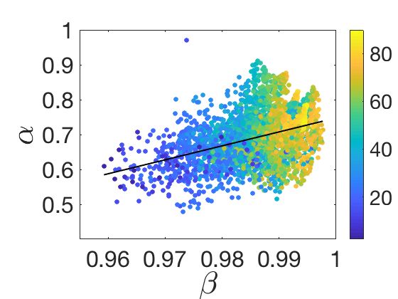
correlate with the corresponding DFA exponents α for all MEG sensors and subjects.
the critical point (Fig 2D and Fig S8). Even though all analyzed signals are bandpass-
limited to a central frequency around 10 Hz by filtering, closeness to criticality appears
to strongly correlate with the fraction of total power in the raw signal in the alpha band
7(R2 = 0.59; p < 0.001). This suggests that alpha oscillations may be closely related to
critical brain tuning during the resting state [49, 42, 62, 76, 56].
A classic fingerprint of tuning to criticality is the emergence of long-range temporal
correlations (LRTC), which have been documented empirically [49, 42, 62, 13, 57, 56, 52].
LRTC in the alpha band have been investigated primarily by applying the detrended
fluctuations analysis (DFA) to the amplitude envelope of MEG or EEG signals in the
alpha band (SI Appendix) [49, 68, 62, 72]. Briefly, DFA estimates the scaling exponent α
of the root mean square fluctuation function F in non-stationary signals with polynomial
trends [64]. For signals exhibiting positive (or negative) LRTC, F scales as F ∝ nα with
0.5 < α < 1 (or 0 < α < 0.5, respectively); α = 0.5 indicates the absence of long range
correlations; α also approaches unity for a number of known model systems as they are
tuned to criticality [33, 32].
To test for the presence of LRTC using DFA, we analyzed the scaling behavior of
fluctuations and extracted their scaling exponent α [49, 42]. To avoid spurious correlations
introduced by signal filtering, α was estimated over the range 2 s < n < 60 s (Fig 2E) [49,
42]. We find that α is consistently between 0.5 and 1 for all MEG sensors and subjects,
in agreement with previous analyses [49, 59, 62, 87, 57, 13]. Importantly, model-free α
values measured across MEG sensors positively correlate with the inferred β values from
the model (Fig 2F), indicating that higher β values are diagnostic about the presence of
long-range temporal correlations in the amplitude envelope.
Taken together, our analyses so far show that the adaptive Ising model recapitulates
single MEG sensor dynamics by matching their autocorrelation function and the distri-
bution of amplitude fluctuations, and further suggest that the true MEG signals are best
reproduced when the adaptive Ising model is tuned close to, but slightly below, its critical
point (β . 1).
Scale invariant collective dynamics of extreme events
We now turn our attention to phenomena that are intrinsically collective: (i) coordi-
nated supra-threshold bursts of activity, which emerge jointly with LRTC in alpha oscil-
lations [68, 62]; and (ii) neuronal avalanches, i.e., spatio-temporal cascades of threshold-
crossing sensor activity, which have been identified in the MEG of the resting state of the
human brain [76, 56]. Both of these phenomena are generally seen as chains of extreme
events that are diagnostic about the underlying brain dynamics [37, 79, 50, 7, 35, 53].
We start by defining the instantaneous network excitation, A (t), as the number of
extreme events co-occurring within time bins of size across the entire MEG sensor array.
For each sensor, extreme events are the extreme points in that sensor’s signal that exceed
a set threshold e (Fig 3A). For a given threshold, network excitation A depends on the
size of the time bin that we use to analyze the data (Fig 3B). To make contact with
the model, we parcel our simulated network into K equally-sized disjoint subsystems of
nsub = N/K neurons each, and consider each subsystem activity mµ , µ = 1, . . . , K, as
8the equivalent of a single MEG sensor signal. Network excitation, A , for the model then
follows the same definition as for the data, allowing us to perform direct side-by-side
comparisons of extreme event statistics.
We first study the distribution of network excitation, P (A ). We set e = 2.9SD both
for MEG data and for the model [76]. Even though P (A ) generally depends on , the
distributions corresponding to different collapse onto a single, non-exponential master
curve when A is rescaled by γ , with γ = 1/2, for the average over subjects as well as
for individual subjects (Fig 3C). Excitation distribution is thus invariant under temporal
coarse-graining and the number of extreme events scales non-trivially with , in contrast
to phase-shuffled surrogate data (SI Appendix). Remarkably, model simulations fully
recapitulate this data collapse as well as the non-exponential extreme event statistics.
Periods of excitation (A 6= 0) are separated by periods of quiescence (A = 0) of
duration I = n, where n is the number of consecutive time bins with A = 0. The dis-
tribution of quiescence durations, P (I ), is also invariant under temporal coarse-graining
when rescaled by , collapsing onto a single, non-exponential master curve (Fig 3D). Fur-
thermore, we show that the overall probability P0 () of finding a quiescent time bin follows
a non-exponential relation P0 () = exp −aβI , with βI ' 0.6 (Fig 3D, lower inset), indi-
cating that extreme events grouped into bins of increasing size are not independent [58].
The model correctly reproduces the bulk of the distribution of quiescence durations P (I )
and the scaling of P0 (), but it overestimates the fraction of short quiescence periods and
thus the total probability of quiescence, pointing to interesting directions for future work.
These results are independent of the N and nsub so long as the number of subsystems
K is fixed or does not change considerably (Figs S12–S14); otherwise, the threshold e
that defines an extreme event should be adjusted accordingly (Fig S15), in particular to
closely reproduce the distribution of quiescence durations P (I ) (Fig S15).
In sum, our simple model at baseline parameters provides a robust account of the
collective statistics of extreme events. We emphasize that the excellent match to the
observed long-tailed distributions is only observed for the inferred value β ' 0.99 very
close to criticality; already for β = 0.98, we observe significant deviations from data (Figs
S9, S10), demonstrating that excitation and quiescence distributions represent a powerful
benchmark for collective brain activity.
Scale-free neuronal avalanches occur concomitantly with oscillations
A neuronal avalanche is a maximal contiguous sequence of time bins populated with at
least one extreme event per bin (Fig 4A) [11, 76]; every avalanche thus starts after and ends
with a quiescent time bin (A = 0). Typically, neuronal avalanches are characterized by
their size s, defined as the total number of extreme events within the avalanche. Avalanche
sizes have been reported to have a scale-free power-law distribution [11, 66, 76, 36, 56].
We estimate the distribution P (s) of avalanche sizes in the resting state MEG, and
compare it with the distribution obtained from model simulation at close-to-critical base-
9A B ε1 ε2
Amp (SD)
Amplitude (SD)
Sensor number
Sensor number
3 250 250
200 200
0 150 150
100 100
-3 50 50
0 250 500 750
Time (ms) 250 ms Time (ms) Time (ms)
Sensor
ε1 0 1 4 0 1 10 12 4 0 0
ε2 1 4 11 16 0
..
ε10 32
C 10
0
0
10 D 10
0
10
-1
γ
P(Iε)/ε
P(Aε)/ε
-3
10
-2 10
-2 -2 -5
10 -4 10 10
γ
10
P(Aε)/ε
P(Iε)/ε
-7
0 10 20 30 40 10 1 2 3
γ 10 10 10
-4 ε2 = 2T ε Aε -4 MEG ε Iε
10 ε4 = 4T 10 Model 0
10
-lnP0
ε6 = 6T
-6 ε8 = 8T MEG Model -6 -1
10 10
ε10=10T Surrogate 10 1 ε 10
0 10 20 30 40 50 10
0
10
1
10
2
10
3
10
4
γ
ε Aε ε Iε
Figure 3: Non-exponential extreme event statistics in MEG resting state ac-
tivity are reproduced by a marginally subcritical adaptive Ising model. (A)
Extreme events on a single sensor are defined as extreme signal excursions (top; red dots)
crossing a threshold e = ±nSD (horizontal lines). Resulting raster of extreme events
shown across 273 MEG sensors of a single subject across approximately 500 ms recording
(bottom). (B) Events are grouped together in temporal bins n = nT in multiples of
the sampling interval T (top), to define instantaneous network excitation A , the total
number of extreme events across all sensors in a time bin. Representative sequences of
network excitation extracted from the raster in the top panel for increasing bin size n
(bottom). (C) Rescaled distribution of network excitation, P (A ), for e = 2.9SD and a
range of bin sizes n (different plot symbols) in MEG data (green symbols; average over
subjects) and in the model simulated at baseline parameters with K = 100 subsystems
of nsub = 100 neurons each (violet symbols). Distributions for different collapse onto
a single non-exponential master curve for both data and model. Corresponding distri-
bution in phase-scrambled MEG signals shows an exponential behavior, with absence of
high excitation events (brown = surrogate data). Inset: Rescaled P (A ) shown for a
single subject. (D) Rescaled distributions of quiescence durations, P (I ) collapse onto a
single master curve for different . Plotting conventions and model simulation details are
the same as in (C). Top inset: Rescaled P (I ) shown for a single subject. Bottom inset:
Probability P0 of finding a quiescent time bin scales approximately as P0 = exp −aβI
with bin size ; βI = 0.567±0.012 and βI = 0.630±0.005 for data and model, respectively;
βI = 0.996 ± 0.001 for surrogate data.
line parameter set (Fig 4B). Both distributions are described by a power-law with an
exponential cutoff [76] and show an excellent match across subjects and for individual
subjects (Fig 4B, upper inset). Phase scrambled surrogate data strongly deviate from
the power-law observations, as do model predictions when parameter β is moved even
marginally below 0.99 (Fig S11). Importantly, the model also reproduces the scaling re-
10lation hsi(d) ∼ dζ that connects average avalanche sizes s and durations d. Unlike the
power-law exponent of avalanche size distribution that typically depends on time bin size
[11, 56], the exponent ζ does not depend on , as shown by the data collapse for both
MEG data and model (Fig 4B, the inset). While the scaling behavior is reproduced qual-
itatively, the inferred and model-derived values of ζ are not in quantitative agreement,
likely due to the overly simplified mean-field connectivity assumed by our model.
A ε m
Aϵ(i)
Sensor number
∑
250 Size : s =
200
150 i
100 #(active sensors)
50
Duration : d = nε
Avalanche
Time (ms)
B MEG Model -1
10
Surrogate
P(s)
-1
10 -3
10
-5
10
P(s)
0 1 2
10 10 10
-3 Model s
(d)
4
10 10
2
10
0 MEG
10
0 2
-5 10 ε−3/2d 10
10
0 1 2 3
10 10 10 10
s
Figure 4: Scale-free neuronal avalanches in MEG resting state activity are
reproduced by a marginally subcritical adaptive Ising model. (A) Schematic
representation of a neuronal avalanche. Avalanche size s is the sum of network excitations
A over time bins belonging to the avalanche; its duration d is the number of bins times
their duration, . (B) Distribution of avalanche sizes, P (s), for MEG data (green curve
= average over subjects) and the model simulated at baseline parameters with K = 100
subsystems of nsub = 100 neurons each (violet dots). Both distributions are estimated
using a threshold e = 2.9SD and bin size 4 = 4T . Top inset: P (s) for an individual
subject (brown = surrogate data as in Fig 3). Bottom inset: Average avalanche size
scales with its duration as hsi ∼ dζ (different plot symbols = different as in Fig 3;
green = MEG data; violet = model simulation; model simulation curves are vertically
shifted for clarity), so that the exponent ζ remains independent of the time bin size .
ζ = 1.28 ± 0.01 for MEG data (dashed line) and ζ = 1.58 ± 0.03 for model simulation
(thick line).
11Discussion
In this paper, we put forward the adaptive Ising class of models for capturing large scale
brain dynamics. Quite generally, these models combine a microscopic and stochastic
description of excitatory neuron spiking with coarse-grained mean-field model of activity-
dependent feedback. This endows the models with several unique characteristics that we
discuss in turn: (i) the ability to generate a diverse range of stylized behaviors observed
in real brain dynamics and locate these behaviors in the model’s phase diagram; (ii) the
possibility to connect the model to a wide range of known theoretical results in statistical
physics and theoretical neuroscience; (iii) the ability to rigorously infer model parameters
from data, quantitatively test its predictions across a range of spatial and temporal scales,
and thus derive biological insight about brain function.
Diversity of dynamical behaviors in a simple non-equilibrium model
By combining local interactions with a time-varying field in the form of an activity-
dependent feedback, the adaptive Ising model exhibits a phase transition to a self-oscillatory
behavior at the Andronov-Hopf bifurcation critical point that inherits the characteristics
of the classical Ising ferromagnet second-order phase transition [27]. In proximity and
slightly below the critical point, the ongoing network activity m — the equivalent of the
Ising magnetization — shows intermittent oscillations, whose associated reversal time and
zero crossing area are power-law distributed. To our knowledge, this is the simplest model
class that reproduces the stylized coexistence of neuronal avalanches and oscillations, the
two antithetic features of real brain dynamics. Moreover, these features coexist already
in the most basic, mean-field formulation of the model, whose phase diagram can be com-
puted analytically. Interestingly, in this formulation, individual units are neither intrinsic
oscillators themselves [28, 16], nor are they mesoscopic units operating close to a Hopf
bifurcation [39, 28, 22], and the collective dynamics is therefore not a result of oscillator
synchronization (even though this regime can be captured as well by a different realisa-
tion of an adaptive Ising model). Our proposal thus provides an analytically-tractable
alternative to—or perhaps a reformulation of—existing models [68, 29, 36, 26], which
typically implicate particular excitation/inhibition or network resource balance to open
up the regime where oscillations and avalanches may coexist.
Connections to results in statistical physics
Starting with the seminal work of Hopfield [44], the functional aspects of neural networks
have traditionally been studied with microscopic spin models or attractor neural networks.
These systems qualitatively reproduce the associative memory functionality ascribed to
real neural networks [3] and their phase transitions have been thoroughly studied with
statistical mechanics tools [4]. The associated inverse (maximum entropy) problem re-
cently attracted great attention in connecting spin models to data [75, 81], in particular
12with regard to criticality signatures [82]. One of the major shortcomings of these models
is their implied equilibrium dynamics [73], within which the rhythmic behavior of brain
oscillations is impossible to reproduce. Adaptive Ising model class can be seen as a nat-
ural extension to the previous work that enables oscillations and furthermore permits us
to explore an interesting interplay of mechanisms, for example, by having self-feedback
drive Hopfield-like networks (with memories encoded in the coupling matrix J) through
sequences of stable states.
Another link to rich existing literature becomes apparent when we consider connec-
tivity degrees of freedom (encoded in J and in the pooling that drives the feedback;
SI Appendix) in order to model cell types (e.g., inhibitory vs excitatory), the spatial
structure of the cortex, or to capture empirically established topological features of real
neural networks. Within equilibrium statistical mechanics, the effects of various lattices
or disordered connectivity in spin systems have been studied rigorously; phenomenolog-
ical arguments suggest that adding the feedback that drives the adaptive Ising model
out of equilibrium does not change the fundamental nature (e.g., critical exponents) of
the critical point. This permits us to directly translate existing equilibrium results into
the non-equilibrium setup: an example would be the introduction of scale-free topology
among excitatory neurons into our model (example in the SI Appendix). Looking towards
the future, powerful tools of statistical physics, such as the Landau-Ginzburg theory and
the renormalization group, can be brought to bear on the generalizations of the non-
equilibrium adaptive Ising model, enabling rapid progress based on existing equilibrium
results.
Inferring the model to derive biological insights
Since the adaptive Ising model can be solved analytically in the mean field limit, we can
infer its two key parameters by matching the auto-correlation function of MEG signals
to the model-predicted auto-correlation function. In contrast to previous work [29, 68],
we do not make contact with existing data by qualitatively matching the phenomenology,
but by proper parameter inference. The inferred parameters consistently place the model
very close to its critical point, supporting the hypothesis that alpha oscillations represent
brain tuning to criticality [49, 38, 42, 39, 62]. The possibility of mapping empirical
data to a defined region in the adaptive Ising model phase diagram through parameter
inference paves the way for further quantification of the relationship between measures of
brain criticality and healthy, developing, or pathological brain dynamics along the lines
developed recently [34, 87, 7].
Our inferred model makes a wide range of further predictions that can be confronted
with data. By parcelling the simulated system into groups of spins, we can mimic the sig-
nals captured by multiple MEG sensors over the cortex. We find a remarkable quantitative
correspondence between the non-exponential and scale-invariant distribution of network
excitation observed across the MEG sensors and in our simulation, which holds when
13averaged across individuals or within single individuals. Even though the distribution of
quiescent periods is not matched with the quantitative precision we observe for network
excitation, our analysis clearly demonstrates that extreme events are non-independent
across space and time. This non-trivial spatio-temporal organization of extreme events is
strongly indicative of a network state close to criticality [79, 37]; the agreement between
model and data breaks down for surrogate data as well as for models further removed
from criticality. Moreover, the extreme events coalesce into neuronal avalanches as re-
ported previously [11, 66, 76, 56], which our model reproduces as well. Taken together,
our model provides a remarkably broad account of brain dynamics across spatial and
temporal scales.
Despite these successes, we openly acknowledge the quantitative failures of our model:
(i) at the single sensor level, small deviations exist in the distributions of log activ-
ity (Fig 2C), likely due to very long timescales or non-stationarities in the MEG sig-
nals [76, 78, 77]; (ii) significant deviations exist in the probability distribution for short
quiescent intervals even when its tail is reproduced very well (Fig 3D); (iii) the scaling
exponent governing the relation between the avalanche size and duration, ξ, is not repro-
duced quantitatively (Fig 4B, inset). Furthermore, beyond the two key model parameters
that were inferred directly from individual sensors (β, c), quantitative data analysis of
extreme events requires additional parametric choices (time bin , threshold e, system
size N and subsystem size nsub ), both for empirical data as well as model simulations.
While we successfully demonstrate the scaling invariance of the relevant distributions with
respect to and robustness with respect to N and nsub at fixed N/nsub , a close match to
data still requires choosing one extra parameter (e.g., threshold e).
Despite these valid points of concern, we find it remarkable that such a simple and
tractable model can quantitatively account for so much of the observed phenomenology.
Future work should first consider connectivity beyond the simple all-to-all mean-field
version that we introduced here, likely leading to a better data fit and new types of
dynamics, e.g, cortical waves. Second, we strongly advocate for rigorous and transparent
data analysis and quantitative—not only stylized—comparisons to data. To this end,
care must be taken not only when inferring the essential model parameters, but also to
deal properly with the hidden “degrees of freedom” related to data analysis (related to
subsampling, temporal discretization, thresholding etc.) [70, 48, 11, 56, 76]. Third, it is
important to confront the model with different types of brain recordings; a real success in
this vein would be to account simultaneously for the activity statistics at the microscale
(spiking of individual neurons) as well as at the mesoscale (coarse-grained activity probed
with MEG, EEG, or LFP).
14Supplementary Information
Methods
Data acquisition and pre-processing
Ongoing brain activity was recorded from 14 healthy participants in the MEG core facility
at the NIMH (Bethesda, MD, USA) for a duration of 4 min (eyes closed). All experiments
were carried out in accordance with NIH guidelines for human subjects. The sampling
rate was 600 Hz, and the data were band-pass filtered between 1 and 150 Hz. Power-line
interferences were removed using a 60 Hz notch filter designed in Matlab (Mathworks).
The sensor array consisted of 275 axial first-order gradiometers. Two dysfunctional sen-
sors were removed, leaving 273 sensors in the analysis. Analysis was performed directly
on the axial gradiometer waveforms. The data analyzed here were selected from a set of
MEG recordings for a previously published study [76]. For the present analyses we used
the subjects showing the highest percentage of spectral power in the alpha band (8-13
Hz). Similar results were obtained for randomly selected subjects.
Adaptive Ising model: further details
The model is composed of a collection of N spins si = ±1 (i = 1, 2, ..., N ) that interact
with each other with a coupling strength Jij . In our analysis, the N spins represent ex-
citatory neurons that are active when si = +1 or inactive when si = −1, and Jij > 0.
Furthermore, we consider the fully homogeneous scenario, with neurons interacting with
each other through synapses of equal strength Jij = J = 1. However, interesting gen-
eralization with non-homogeneous, negative, non-symmetric Jij are possible, to include,
for example, the effect of inhibitory neuronal population and structural and functional
heterogeneity. The si are stochastically activated according to the Glauber dynamics,
where the state of a neuron is drawn from the marginal Boltzmann-Gibbs distribution
X
P (si ) ∝ exp(β h̃i si ) h̃i = Jij sj + hi (4)
j
The spins experience an external field h, a negative feedback that depends on network
activity according to the following equation,
|Ni |
1 X
ḣi = −c sj , (5)
|Ni |
j∈Ni
where c is a constant that controls the feedback strength, and the sum runs over a neigh-
borhood of the neuron i specified by Ni ; index j enumerates over all the elements of this
neighborhood. Depending on the choice of Ni , the feedback may depend on the activity of
the neuron i itself (self-feedback), its nearest neighbors, or the entire network — the case
15we considered in the main paper. In a more realistic setting including both excitatory
(Jij > 0) and inhibitory neurons (Jij < 0), one could then take into account the different
structural and functional properties of excitatory and inhibitory neurons by considering
different interaction and feedback properties [14]. In our simulations, one time step cor-
responds to one system sweep — i.e. N spin flips — of Monte Carlo updates, and Eq (5)
is integrated using ∆t = 1/N . Note that this choice of timescales for deterministic vs
stochastic dynamic is important, as it interpolates between the quasi-equilibrium regime
where spins fully equilibrate with respect to the field h, and the regime where the field
is updated by feedback after each spin-flip and so spins can constantly remain out of
equilibrium. ∆t is generally much smaller than the characteristic time of the adaptive
feedback that is controlled by the parameter c.
Mapping between the adaptive Ising model and an EI network
We first encode a classic E-I model that leads to sustained oscillations, into an Ising
model framework. We can think of this model as a single network of N units whose
coupling matrix Jij is asymmetric and is structured into two blocks that correspond to
an excitatory and an inhibitory subpopulation. Specificcally, the network consists of a
population 1, which is self-exciting with strength J11 and which excites population 2 with
strength J12 , while population 2 is inhibiting population 1 with strength J21 .
It can be demonstrated that the mean-field dynamics of this stochastic system of
Ising-like neurons in the limit of large populations is described by a Liouville deterministic
equation of the form (mi i = 1, 2 is the average spiking rate of population i) [17]:
ṁ1 = −m1 + tanh(J11 m1 + J21 m2 ) (6)
ṁ2 = −m2 + tanh(J12 m2 ) (7)
(8)
The E-I network has an ergodic state where (m1 = m2 = 0). Stability analysis to small
perturbations of this state reveals an Andronov-Hopf bifurcation towards self-oscillations,
when J11 = 2 and −J12 J21 > 1. Upon matching the coefficients of such a linear expansion:
m̈ + (1 − β)ṁ + cβm = 0 (9)
m̈1 + (2 − J11 )ṁ1 + (1 − J11 − J12 J21 )m1 = 0 (10)
we get an approximate mapping into the parameters β, c of the simplest adaptive Ising
model:
J11 = β + 1 (11)
p
J12 = β(1 + c) (12)
p
J21 = − β(1 + c) (13)
16.
The role of topology
One of the most interesting questions about synchronization in neural networks is how
general features of the interaction topology affect the collective behavior, i.e., how struc-
ture affects function in general terms [18]. From a modeling perspective, most efforts have
focused on studying the Kuramoto model (KM) [6], where the individual excitable units
are already postulated to be oscillators (for a discussion about this point see [5]). Never-
theless, no exact analytical results for the KM on general networks are available up to now,
with an intense debate currently focusing on the nature of the onset of synchronization
in strongly heterogeneous topologies [65].
In contrast, we provide here an heuristic argument that the adaptive Ising model
directly inherits the wealth of knowledge accumulated about its equilibrium counterpart,
in particular, with regard to the features and the location of its critical point(s). The
critical point characteristics have been rigorously determined in several geometries, from
dimensional lattices to complex networks and small world [61, 10, 31].
The fact that equilibrium Ising results can be generalized to the adaptive case can
be seen directly from the application of the linear response theory, upon considering
the Landau expression for the free energy: by construction, the bifurcation point of the
dynamical model coincides with the critical point of the underlying equilibrium model.
For instance, for the case of uncorrelated tree-like random graphs, described by a
degree distribution P (k) [60], the linear response applied to a Curie-Weiss approximate
expression for the free energy [47] leads to the following approximate dynamical equations
for the firing rates of nodes with degree k, mk (where hki is the mean degree, hmi =
P P k
k P (k)mk is the average firing rate and hmv i = k hki P (k)mk is the average firing rate
upon following a random link):
ṁk = −mk + tanh(β(khmv i + h)) ∀k (14)
ḣ = −chmi. (15)
As it can be easily verified by linearizing around the stationary solution mk = h = 0,
these equations show that the model has a bifurcation point located at the same position
hk2 i
as the equilibrium critical point, i.e. (βJ)c = hki (a more refined calculation [47] based
hki
on asymptotically exact Bethe-Peierls approximation gives (βJ)c = − 12 log(1 − 2 hk 2 i )).
This simple example shows that the inverse temperature gets renormalized by the
hk2 i
branching ratio [60] hki , a topological measure of the density of links, or synaptic con-
nections in our context, that could be considered itself as the key control parameter
driving the system in and/or out the synchronized phase. A direct consequence for our
case is that if the topology we were considering were scale free, i.e. with an heavy tail
for the degree distribution P (k) ∼ k −γ γ < 3, then βc → 0 and the system would always
17be in the synchronized phase, a feature shared by many collective phenomena in strongly
heterogeneous networks [31]. In our case, subcritical dynamics is inferred from data and
the scale-free topology is not appropriate, but the reasoning here demonstrates clearly
how known facts about equilibrium Ising on different topologies can directly translate
into the insights of the adaptive Ising model.
Detrended Fluctuations Analysis of the alpha band amplitude envelope
The DFA [64] consists of the following steps: (i) Given a time series xi (i = 1, ..., N )
calculate the integrated signal I(k) = ki=1 (x(i)− < x >), where < x > is the mean of
P
xi ; (ii) Divide the integrated signal I(k) into boxes of equal length n and, in each box, fit
I(k) with a first order polynomial In (k), which represents the trend in that box; (iii) For
each n, detrend I(k) by subtracting the local trend,
qP In (k), in each box and calculate the
N 2
root-mean-square (r.m.s.) fluctuation F (n) = k=1 [I(k) − In (k)] /N ; (iv) Repeat this
calculation over a range of box lengths n and obtain a functional relation between F (n)
and n. For a power-law correlated time series, the average r.m.s. fluctuation function
F (n) and the box size n are connected by a power-law relation, that is F (n) ∼ nα .
The exponent α quantifies the long-range correlation properties of the signal. Values of
α < 0.5 indicate the presence of anti-correlations in the time series xi , α = 0.5 absence of
correlations (white noise), and α > 0.5 indicates the presence of positive correlations in
xi . The DFA was applied to the alpha band (8 − 13 Hz) amplitude envelope. Data were
band filtered in the range 8-13 Hz using a FIR filter (second order) designed in Matlab.
The scaling exponent α was estimated in the n range corresponding to 2s - 60s to avoid
spurious correlations induced by the signal filtering [49, 42].
Definitions: Extreme events, instantaneous network excitation A , neu-
ronal avalanches
For each MEG sensor, positive and negative deflections in the MEG signal were detected
by applying a threshold e at ±2.9 standard deviations (SD). In each excursion beyond the
threshold, a single event was identified at the most extreme value (maximum for positive
excursions and minimum for negative excursions). The raster of events was binned at a
number of temporal resolutions , which are multiple of the sampling time T = 1.67 ms.
The network excitation A at a given temporal resolution is defined as the number of
events occurring across all sensors in a time bin. An avalanche is defined as a continuous
sequence of time bins in which there is at least an event on any sensor, ending with at
least a time bin with no events (Fig 4A). The size of an avalanche, s, is defined as the
number of events in the avalanche. For further details see [76, 56].
18Surrogate data
Surrogate signals are obtained by random phase shuffling of the original continuous MEG
signals. A Fourier transform of each sensor signal is performed, the corresponding phases
are randomized while amplitudes are preserved. The surrogate signals are then obtained
by performing an inverse Fourier transform. The random phase shuffling destroys phase
synchronization across cortical sites while preserving the linear properties of the original
signals, such as power spectral density and two-point correlations [80].
Acknowledgements
FL acknowledges support from the European Union’s Horizon 2020 research and inno-
vation program under the Marie Sklodowska-Curie Grant Agreement No. 754411. GT
acknowledges the support of the Austrian Science Fund (FWF) under Stand-Alone Grant
No. P34015.
19A 1.2 C
c = 0.5 0.02
0.6 c=2
c = 10
m
C
0
0
-0.02
-0.6
0 10 20 0 100
B t/tc D t/tc
0.02 0.02
m
m
0 0
-0.02 -0.02
0 100 0 100
t/tc t/tc
Figure 5: Autocorrelation C and ongoing network activity m for β = 0.5 and different
c values. Far from the critical point, the presence of a strong adaptive feedback may
also produce short — C rapidly decays to zero — intermittent oscillation bursts. (A)
Autocorrelation for different c values. (B) m for c = 0.5. (C) m for c = 2. (D) m for
c = 10. tc is the inferred autocorrelation time from exponential fit.
20A β = 0.5 C β=1
0.02 1.8 0.1
0.8
m
m
0 0
-0.02 1.2 -0.1
A(τ)
A(τ)
t 0.6 t
C
C
0.4
0
0 -0.6
0 20 40 60 0 40 80
τt τt
B β = 0.75 D β = 1.1
1.8 0.08
2 0.4
m
m
0 0
1.2 -0.4
A(τ)
A(τ)
-0.08
t 1 t
C
C
0.6
0 0
-0.6
-1
0 40 80 0 40 80
tτ τt
Figure 6: The autocorrelation C and ongoing network activity m for c = 0.5 and different
values of the parameter β controlling proximity to the critical/bifurcation point βc . In
all cases the system is the resonant regime, and well above the transition line c = c∗ .
However, we observe that the system only develops consistent and structured oscillations
for large enough β values, namely closer to the critical point β = 1. For β > 1, the system
exhibits self-oscillations.
A 10
1 B -1
10
-1
10
P(a0)
P(t)
-3
10
-3 10
c = 10-5 c = 10-5
10
-5 c = 10-3 -5 c = 10-3
c = 10-2 10 c = 10-2
-7
10 -2 -1 0 1 2 3 0 1 2 3
10 10 10 10 10 10 10 10 10 10
a0 t
Figure 7: The reversal time t is defined as the time interval between consecutive zero-
crossing events in the ongoing network activity m (Fig. 1). The quantity a0 is the area
under the curve between two zero-crossing events. (A) Distribution P (a0 ) of the quantity
a0 for the model at the critical point β = 1 for the different strengths c of the adaptive
feedback. (B) Distribution P (t) of the reversal time for β = 1 and different values of the
parameter c.
211 m
0.1
0
0.5 t
C
β = 0.9, c = 0
0
0 50 100
τ
Figure 8: The autocorrelation C and ongoing network activity m (inset) without adaptive
feedback, i.e. c = 0. Even though β is close to the critical value β = 1, the network does
not exhibit any oscillatory behavior.
221 Broadband
0
C
MEG Model
-10 100 200 300
t
2 MEG Broadband
Amp (SD)
0
-2
2 Model
0
-2
0 500 1000 1500
Time (ms)
Figure 9: (Top panel) Broadband MEG signal autocorrelation and corresponding model
autocorrelation for inferred parameters. (Bottom panel) The broadband signal from a
single MEG sensor in the resting awake state is compared with the network activity m
from model simulations with parameters β = 0.99 and c = 0.01 inferred from the single
sensor signal.
230.6 MEG
β = 0.7
P(log ae)
0.4 β = 0.98
β = 0.99
0.2
0
-6 -4 -2 0 2
log(ae)
Figure 10: Distributions P (log ae ) of the logarithm of the area under the curve ae , with
e = 2.5SD, for MEG data (green curves = average over sensors for one subject) and the
model with different β values and c = 0.5.
0.6 MEG
Model
P(log ae)
0.4
0.2
0
-6 -4 -2 0 2
log(ae)
Figure 11: Distributions P (log ae ) of the logarithm of the area under the curve ae , with
e = 2.5SD, for MEG data (green curves = average over sensors for one subject) and the
model with corresponding inferred parameter values.
24A B
0.03
0.1
P(c)
0.1
0.02
P(β)
P
0
0.01 0.012 0.014
0.01
c
0
0.014
0.99 0.012 0
0.98 0.96 0.98 1
0.97 0.01 c
0.96 β
Figure 12: (A) Joint probability of inferred values of the two model parameters from
all MEG sensors (273) and subjects (14). (B) Marginal probability distributions of the
inferred model parameters β (main panel) and c (inset).
0
10
MEG
β = 0.70
β = 0.95
-2
β = 0.98
γ
10
P(Aε)/ε
β = 0.99
-4
10
-6
10 0 10 20 30 40 50 60
γ
ε Aε
Figure 13: Distributions of the activity per bin A for different values of β in model
simulations with N = 104 spins, and for MEG data (average over subjects). The model
network is parceled in 100 disjoint subsystems, each including 100 spins. In all cases the
model is in the resonant regime. The activity per bin A is rescaled by γ with γ = 0.5,
and 2 = 2T , where T is the sampling interval. β = 0.99 corresponds to the average β
value inferred from MEG data.
25You can also read