Magnetosheath jet evolution as a function of lifetime: global hybrid-Vlasov simulations compared to MMS observations
←
→
Page content transcription
If your browser does not render page correctly, please read the page content below

Ann. Geophys., 39, 289–308, 2021
https://doi.org/10.5194/angeo-39-289-2021
© Author(s) 2021. This work is distributed under
the Creative Commons Attribution 4.0 License.

Magnetosheath jet evolution as a function of lifetime:
global hybrid-Vlasov simulations compared to MMS observations
Minna Palmroth1,2 , Savvas Raptis3 , Jonas Suni1 , Tomas Karlsson3 , Lucile Turc1 , Andreas Johlander1 , Urs Ganse1 ,
Yann Pfau-Kempf1 , Xochitl Blanco-Cano4 , Mojtaba Akhavan-Tafti5 , Markus Battarbee1 , Maxime Dubart1 ,
Maxime Grandin1 , Vertti Tarvus1 , and Adnane Osmane1
1 Department   of Physics, University of Helsinki, Helsinki, Finland
2 Space  and Earth Observation Centre, Finnish Meteorological Institute, Helsinki, Finland
3 KTH Royal Institute of Technology, Stockholm, Sweden
4 Instituto de Geofisica, Universidad Nacional Autonoma de Mexico, Mexico City, Mexico
5 Climate and Space Science and Engineering, University of Michigan, Ann Arbor, USA

Correspondence: Minna Palmroth (minna.palmroth@helsinki.fi)

Received: 3 July 2020 – Discussion started: 15 July 2020
Revised: 1 February 2021 – Accepted: 2 February 2021 – Published: 12 March 2021

Abstract. Magnetosheath jets are regions of high dynamic            namic pressure and magnetic field intensity as compared to
pressure, which can traverse from the bow shock towards the         the jets during high MA .
magnetopause. Recent modelling efforts, limited to a single
jet and a single set of upstream conditions, have provided the
first estimations about how the jet parameters behave as a
function of position within the magnetosheath. Here we ex-          1   Introduction
pand the earlier results by doing the first statistical investi-
gation of the jet dimensions and parameters as a function of        Earth’s magnetosheath is a region of turbulent shocked
their lifetime within the magnetosheath. To verify the simu-        plasma of solar wind origin. The earthward boundary of the
lation behaviour, we first identify jets from Magnetosphere         magnetosheath is the magnetopause, while the outer bound-
Multiscale (MMS) spacecraft data (6142 in total) and con-           ary is the bow shock, at which the characteristics of the solar
firm the Vlasiator jet general behaviour using statistics of 924    wind plasma abruptly change. Many of the magnetosheath
simulated individual jets. We find that the jets in the simula-     global properties can be predicted from gas-dynamic or mag-
tion are in quantitative agreement with the observations, con-      netohydrodynamic (MHD) models (e.g. Stahara, 2002; Zas-
firming earlier findings related to jets using Vlasiator. The jet   tenker et al., 2002; Walsh et al., 2012; Dimmock and Nykyri,
density, dynamic pressure, and magnetic field intensity show        2013); for example, the magnetosheath plasma is overall
a sharp jump at the bow shock, which decreases towards the          denser and hotter as compared to the solar wind. Since the
magnetopause. The jets appear compressive and cooler than           bow shock is a fast magnetosonic shock, the magnetosheath
the magnetosheath at the bow shock, while during their prop-        magnetic field is also more intense as compared to the in-
agation towards the magnetopause they thermalise. Further,          terplanetary magnetic field (IMF) (Petrinec, 2013). How-
the shape of the jets flatten as they progress through the mag-     ever, magnetosheath physics is inherently kinetic physics,
netosheath. They are able to maintain their flow velocity and       indicating that many magnetosheath characteristics are ne-
direction within the magnetosheath flow, and they end up            glected in the gas-dynamical and MHD treatments. For ex-
preferentially to the side of the magnetosheath behind the          ample, mirror-mode and Alfvén ion cyclotron waves, excited
quasi-parallel shock. Finally, we find that Vlasiator jets dur-     by temperature anisotropies, are frequently observed in the
ing low solar wind Alfvén Mach number MA are shorter in             magnetosheath (Schwartz et al., 1996; Génot et al., 2009;
duration, smaller in their extent, and weaker in terms of dy-       Soucek et al., 2015; Dimmock et al., 2015; Dubart et al.,
                                                                    2020). Further, the alteration of incoming solar wind param-

Published by Copernicus Publications on behalf of the European Geosciences Union.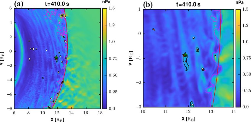
290                                                                          M. Palmroth et al.: Magnetosheath jet statistics

eters in the magnetosheath can depart from MHD predictions         a single jet that was carefully confirmed to represent a jet
(Turc et al., 2017), and there may be other kinetic ion-scale      based on three different observational criteria. They found
features like wave–particle interactions that play a role in       that the investigated single jet was an elongated structure,
the characteristics of the overall magnetosheath (Dimmock          with a length of about 2.6 RE and width of about 0.5 RE . Fur-
et al., 2017). One decisive factor controlling the variabil-       ther, supporting the idea presented by Karlsson et al. (2015),
ity of the magnetosheath in general is the orientation of the      they found that the jet originated at the bow shock in con-
IMF with respect to the bow shock surface (e.g. Lucek et al.,      sequence of a foreshock high dynamic pressure, resembling
2005). The incoming solar wind particles reflect at the bow        a short, large-amplitude magnetic structure (SLAMS; e.g.
shock and propagate far upstream (Schwartz et al., 1983). If       Lucek et al., 2002).
the IMF is approximately quasi-parallel with the shock nor-           In this paper we extend the Palmroth et al. (2018a) investi-
mal, the reflected particles cause instabilities and waves in      gation to incorporate more than one jet in a single simulation
a region called the foreshock upstream of the shock (East-         run. We identify a statistical data set of multiple jets in four
wood et al., 2005). These foreshock waves advect with the          runs with a range of solar wind conditions. We concentrate on
solar wind towards the bow shock and interact with it and          the role of the bow shock normal angle (θBn ) and solar wind
cause increased turbulence and variability within the magne-       Alfvén Mach number MA , since these parameters are chiefly
tosheath downstream of the quasi-parallel shock (Němeček         responsible for influencing the shock properties. Since we
et al., 2002; Shevyrev et al., 2007; Dimmock et al., 2014).        deal with simulation results, we first verify the statistical sim-
   Němeček et al. (1998) provided some of the first obser-       ulation data set by rigorously comparing it to a data set col-
vations of kinetic structures, which are now called magne-         lected from the Magnetosphere Multiscale (MMS) spacecraft
tosheath jets, characterised by high plasma velocities and         (Burch et al., 2016). After confirming that the simulation data
dynamic pressures. Plaschke et al. (2018) present a recent         set is in quantitative agreement with the MMS statistics, we
review of the observational features of the jets and their         investigate the jet properties as a function of time and rela-
statistical characteristics, including their influence on mag-     tive position from the bow shock using the superposed epoch
netospheric dynamics. In summary, jets have been associ-           method. Further, we investigate how the jets travel within the
ated with the quasi-parallel magnetosheath, suggesting that        magnetosheath and where they preferentially end up. The pa-
they originate from interactions between the foreshock and         per is organised as follows: first, we introduce the Vlasiator
the bow shock (e.g. Archer and Horbury, 2013; Plaschke             simulation and the runs that are used, along with introducing
et al., 2013; Vuorinen et al., 2019). Using a large statistical    the MMS data set. We then present an example jet from both
database, Plaschke et al. (2013) further demonstrate that the      data sets and confirm their individual properties, after which
jet durations are around tens of seconds, are faster and more      we compare the properties statistically. Finally, we move to
dense, and have a larger magnetic field intensity relative to      investigate the jet properties as a function of the lifetime and
the ambient magnetosheath. On the other hand, Plaschke             end the paper with our discussion and conclusions.
et al. (2018) note that the jets are commonly colder than
the surrounding magnetosheath. Despite their localised na-
ture, jets play a role in energy transfer from the solar wind to
the magnetosphere, for example in triggering magnetopause          2     Methods
reconnection (Hietala et al., 2018) or magnetopause surface
waves (Archer et al., 2019).                                       2.1    Vlasiator
   Modelling studies of the magnetosheath jets so far have
concentrated on investigating the properties of single jets ap-    We use Vlasiator (Palmroth et al., 2013; von Alfthan
pearing in ion-kinetic simulations. Consistent with observa-       et al., 2014; Palmroth et al., 2018b), which is a global
tional statistics, many modelling studies (e.g. Omidi et al.,      hybrid-Vlasov simulation, propagating protons as distribu-
2016; Palmroth et al., 2018a) associate the jets with the          tion functions while assuming electrons to be a massless
quasi-parallel magnetosheath and foreshock–bow shock in-           charge-neutralising fluid. Vlasiator solves ion-kinetic-scale
teractions. Modelling results of single jets within simulations    physics self-consistently by representing the ions in a three-
show that the jet characteristics, like the dynamic pressure,      dimensional (3D) velocity space grid (3V). The ion distribu-
velocity, and magnetic field intensity, appear within the range    tions are propagated in time using the Vlasov equation, and
of observational statistics. The power of modelling tools in       the velocity space is coupled to the ordinary space, where
investigating the jets is that in simulations single jets can be   electromagnetic fields are solved using Maxwell’s equations
followed in time and that their characteristics can be inves-      and complemented by Ohm’s law including the Hall term.
tigated as a function of the jet lifetime. Further, in observa-    The power of Vlasiator in comparison to the complemen-
tions, the jet length scales can only be inferred from the time    tary particle-in-cell method is that the distribution function
it takes for the jet to traverse over the spacecraft, while in     is noiseless (see, for example, Kempf et al., 2015). While
simulations the jet size can be determined as a function of        Vlasiator’s ordinary space is inherently 3D, in this paper we
time. Palmroth et al. (2018a) showed the first such study for      use a 2D simplification due to the computational resources

Ann. Geophys., 39, 289–308, 2021                                                      https://doi.org/10.5194/angeo-39-289-2021
M. Palmroth et al.: Magnetosheath jet statistics                                                                              291

that were available for the set of runs. This makes the total     of the satellites, all satellites provide comparable measure-
dimensionality of the model here 2D3V.                            ments. The solar wind parameters used to normalise MMS
   We present four different runs carried out in the ecliptic     data are retrieved from the OMNI database (King and Papi-
xy plane in the geocentric solar ecliptic (GSE) coordinate        tashvili, 2005).
system. The simulation box for the different runs varies but
is large enough to include the solar wind, foreshock, dayside
magnetosheath, and parts of the nightside. The resolution is      3   Example jet: modelling and observations
the same for all runs (227 km for the real space and 30 km s−1
                                                                  In earlier jet studies several criteria for defining and identi-
for the velocity space), to the best of our knowledge a break-
                                                                  fying magnetosheath jets were used. For example, Plaschke
through resolution compared to previous hybrid-kinetic sim-
                                                                  et al. (2013) compare magnetosheath dynamic pressure
ulation studies of jets. We have carefully analysed the min-
                                                                  (evaluated using the x component of the ion velocity) to the
imum requirements for spatial and velocity space resolution
                                                                  solar wind dynamic pressure and demand that the former
(Pfau-Kempf et al., 2018; Dubart et al., 2020) and chosen
                                                                  should be at least 25 % of the solar wind pressure. Archer and
the run parameters so that the physics of jets is properly de-
                                                                  Horbury (2013) used only magnetosheath data and defined a
scribed. The inner boundary of the magnetospheric domain
                                                                  jet as an enhancement of the dynamic pressure as compared
is 5 RE for all runs. The ionospheric boundary is a perfectly
                                                                  to the ambient magnetosheath value and defined a “dynamic
conducting circle. The dipole strength has been set to repre-
                                                                  pressure enhancement” by demanding that
sent the natural dipole strength at Earth, indicating that the
modelling results can be given in SI units without scaling.        Pdyn
Each run introduces the solar wind conditions in the sunward              ≥ 2,                                                (1)
                                                                  hPdyn i
wall, while copy conditions are applied in the other walls,
and in the z direction periodical boundary conditions are ap-     where the dynamic pressure is given by Pdyn = ρv 2 using the
plied. The initial velocity distribution is Maxwellian, which     plasma mass density ρ and velocity v. The angular brackets
then changes self-consistently when the runs advance.             in Eq. (1) denote a temporal average, which Archer and Hor-
   Table 1 presents the input parameters for the runs in terms    bury (2013) implemented as a running average with a 20 min
of the solar wind and interplanetary magnetic field (IMF).        window. The benefit of this Archer criterion is that it elimi-
Two of the runs have an IMF cone angle, measured from the         nates the need of solar wind data, which are not always avail-
Sun–Earth line, of 30◦ , while the two others have an almost      able or which may be fluctuating strongly, making it difficult
radial IMF. The solar wind Alfvén Mach number MA within           to decide which data should be used in the normalisation. In
the runs incorporates a spread from 3.4 to 10. The solar wind     this paper we apply the Archer criterion; however, in Vlasia-
values have been chosen to accommodate a variability in the       tor we average over 3 min and keep the 20 min for the MMS
MA , while still having the values well within the range of       data. The 3 min running average centred at the time of in-
typical values (Winterhalter and Kivelson, 1988), justifying      terest in the Vlasiator data was already deemed accurate by
investigations of the foreshock and its interactions with the     Palmroth et al. (2018a), who compared three different jet cri-
bow shock. The run set facilitates investigation of the mag-      teria within the Vlasiator simulation.
netosheath jets in terms of the central parameters in shock          For the MMS statistics, we initially find the time inter-
physics, i.e. the shock normal angle with respect to the IMF      vals in which MMS resides inside the magnetosheath region.
direction (θBn ), and MA . These runs have been used in a va-     This is carried out using thresholds for the ion density, tem-
riety of investigations of the foreshock and magnetosheath        perature, velocity, and flux that are set manually. In addi-
properties (see, for example, Palmroth et al., 2015; Hoilijoki    tion, we require that the magnetosheath interval lasts at least
et al., 2016; Turc et al., 2018, 2019; Palmroth et al., 2018a).   15 min, to avoid possible influence of the bow shock or mag-
                                                                  netopause. After determining the magnetosheath intervals,
2.2   MMS spacecraft and solar wind data                          we use the in situ measurements of ion velocity and den-
                                                                  sity to compute the dynamic pressure and apply the Archer
MMS was launched on 12 March 2015. Since then it has pro-         criterion in Eq. (1) using a 20 min average time window. We
vided measurements using a comprehensive suite of plasma          require that the jet is identified at least 15 min away from the
instruments (Burch et al., 2016). In this work, we use the Fast   magnetopause and the bow shock so that the time average is
Plasma Investigation (FPI) for plasma moment data, taken in       not affected. Furthermore, we impose a minimum time sep-
the Fast Survey mode (with one measurement per 4.5 s) (Pol-       aration between jets, ensuring that sequential jet-like mea-
lock et al., 2016) until May 2019. For magnetic field mea-        surements, which appear less than a minute apart but which
surements, we use Survey mode data (8 s−1 ) from the Flux-        are likely part of the same structure, are treated as a single
gate Magnetometer (FGM; Russell et al., 2016). We exclu-          event. MMS data have been used to investigate jets, for ex-
sively use data from MMS1, since due to the small separation      ample, by Raptis et al. (2020). To match the MMS statistics
of the satellites, multi-spacecraft methods are not necessary     with the solar wind parameters, we time-shifted and averaged
in our mostly statistical analysis. Due to the close spacing      OMNI data for an ideal match to the jets’ observation at the

https://doi.org/10.5194/angeo-39-289-2021                                                   Ann. Geophys., 39, 289–308, 2021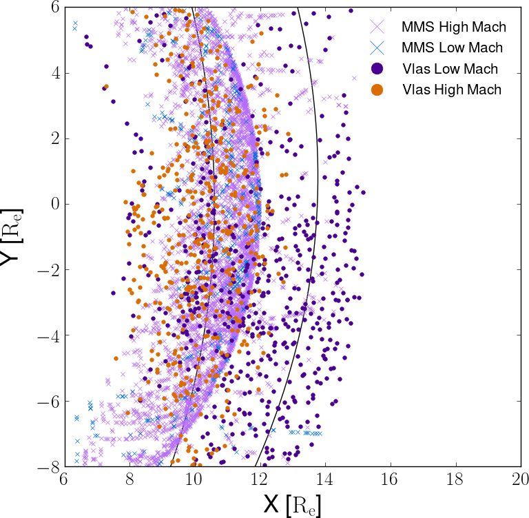
292 M. Palmroth et al.: Magnetosheath jet statistics
Table 1. Characteristics of the four presented runs. The first column gives the run identifier according to the overall run characteristics: H (L)
for high (low) Alfvén Mach number MA and a number giving the interplanetary magnetic field (IMF) cone angle. IMF vector and intensity,
number density n, velocity v, IMF cone angle, and MA are given for all runs. The solar wind temperature for all runs is 0.5 MK. All runs
have the same resolution, 227 km for the real space and 30 km s−1 for the velocity space.
IMF [nT] |IMF| n [cm−3 ] v [km s−1 ] Cone [◦ ] MA
HM30 (−4.3, 2.5, 0.0) 5 1 (−750, 0, 0) 30 6.9
HM05 (−5.0, 0.4, 0.0) 5 3.3 (−600, 0, 0) 5 10
LM30 (−8.7, 5.0, 0.0) 10 1 (−750, 0, 0) 30 3.4
LM05 (−10.0, 0.9, 0.0) 10 3.3 (−600, 0, 0) 5 5
magnetosheath. This was done by taking an average of 20 ripples from being identified as jets, we require that the jets
(1 min resolution) data points from OMNI, starting 15 min are larger than 2 cells (0.05 RE by 0.05 RE ). Hence, Fig. 1a
before the jet observation time and up to 5 min after the jet and b show a black contour delineating jets that are smaller
observation time. This unequal averaging was done because than 4500 cells and larger than 2 cells using the Archer and
the average time from the bow shock to MMS location is Horbury (2013) criterion. Figure 1a and b further show red
∼ 5 min as discussed in Raptis et al. (2020). As a result, by and white dots, which are best visible in Fig. 1b. The red
taking into consideration the time lag, we effectively take a dots give the average centre position of the jets, defined sim-
±10 min window around the associated solar wind measure- ply as the average position of all positions within the con-
ments for the jets. With this technique we remove the ex- tour delineating the jet. The white dots indicate the locations
tremely varying solar wind conditions and take care of the of the largest velocity within the jet. Figure 1a and b show
time shift required from the bow shock to magnetosheath. many jets, most of them appearing near the bow shock sur-
The identification of jets in Vlasiator data is performed as face. Most noticeably, Fig. 1a and b show a jet approximately
follows. Figure 1a and b show a snapshot from run LM30 at [x, y] = [11.8, −1] RE . This jet is investigated in detail in
at time t = 410 s. The full run is presented in the video sup- Fig. 2.
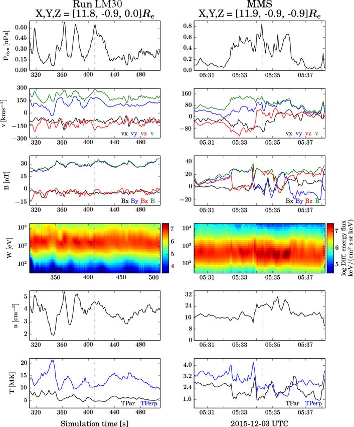
plement, Movie S1 (Suni, 2021). The colour code shows the Figure 2 shows Vlasiator virtual spacecraft and MMS data
dynamic pressure. While the large-scale flow pattern in the from the position shown by the stars in Fig. 1b (orange for
magnetosheath in Vlasiator is as expected, diverging flow Vlasiator and green for MMS). This jet was chosen because
from the Sun–Earth line, the distribution of the velocity mag- its position in Vlasiator and in MMS is at a closest possi-
nitude and the density is more complex due to kinetic pro- ble proximity in all four runs such that the velocity distribu-
cesses arising at the quasi-parallel shock. Thus, the dynamic tion is available within the Vlasiator jet. Although the Vlasia-
pressure within the magnetosheath illustrates remnants of tor simulation solves the velocity space everywhere, it is not
the ultra-low-frequency (ULF) wave fluctuations at the bow written to file everywhere due to restrictions in disk space.
shock, shown as large-scale structures or “stripes” that can The MMS data are gathered on 3 December 2015, during
be seen within the dynamic pressure (see their formation and which the solar wind conditions are the following: velocity
propagation from the bow shock in Movie S1). The red line is around 410 km s−1 , density about 3.8 particles per cubic
shows a fit to the bow shock location, where this position is centimetre, the magnetic field vector about [−4, 3, −2] nT,
defined as the location where the heating of the core popu- and MA ∼ 7. Table 1 presents the solar wind conditions for
lation is larger than 3 times the solar wind temperature, sim- run LM30: velocity is 750 km s−1 , density 1 particle per cu-
ilarly as in Battarbee et al. (2020). Identifying the magne- bic centimetre, magnetic field vector [−8.7, 5, 0] nT, and MA
topause position in these 2D3V runs is complicated (Palm- 3.4. Despite the small difference in the location at which the
roth et al., 2018a), and thus in this paper we concentrate more data are given and the discrepancies in the solar wind condi-
on regions near the bow shock. The magenta contour shows tions, the Vlasiator and the MMS jets show a good temporal
as a reference the regions where the Plaschke et al. (2013) correspondence. The pressure increases in a similar manner
criterion is in force using the 25 % threshold. Figure 1a shows from outside of the jet to within the jet (the vertical dashed
that the Plaschke et al. (2013) criterion identifies large re- black line indicates the peak pressure within the jet). The ve-
gions, particularly towards the flanks as jets. Since these ar- locity and the magnetic field show some discrepancies, such
eas are likely those at which the magnetosheath flow starts to as slower flows and more variable magnetic fields at MMS,
accelerate towards the nightside, and hence not likely jets, in reflecting the differences in the solar wind conditions as well
this paper we use the Archer and Horbury (2013) criterion as the possible different relative positions within the magne-
for identification. We additionally require that the jets are tosheath. The energy spectrogram in Vlasiator is a directional
smaller than 4500 cells, which corresponds to a surface area integral of phase space as a function of energy and time,
amounting roughly to 6 RE by 6 RE . Further, to limit small similar to the method introduced in Jarvinen et al. (2018).
Ann. Geophys., 39, 289–308, 2021 https://doi.org/10.5194/angeo-39-289-2021
M. Palmroth et al.: Magnetosheath jet statistics                                                                                            293

Figure 1. (a) A zoomed-in view of the magnetosheath in Vlasiator run LM30 at time 410 s from the start of the simulation. The colour code
shows the dynamic pressure in units of nanopascal (nPa). The magenta contour shows as a reference the regions where the Plaschke et al.
(2013) criterion is at force using the 25 % threshold. The black contours indicate jets identified with the Archer and Horbury (2013) criterion.
The red line is an approximate fit of the bow shock location. Red dots indicate the average centre position of the jet, while the white dots
show the location of largest velocity. The star refers to the location at which the virtual satellite and MMS data are taken and shown in Fig. 2.
(b) Same as (a) but zoomed in further to show the jets in more detail. The two star positions indicate where data are shown in Fig. 2 (orange
for Vlasiator and green for MMS).

This spectrogram shows similar particle energies to the MMS                and [6, 18; −6, 6] RE for HM05 and LM05 runs. Search ar-
data, slightly larger in Vlasiator because of the larger solar             eas were chosen to focus on the bow shock nose, with addi-
wind velocity. Similarly, the differences in the density and               tional space in the −y direction for the 30◦ cone angle runs
temperature can be understood in terms of the differences                  to capture more of the foreshock, while omitting most of the
in the solar wind parameters. The main purpose of Fig. 2 is                flanks and regions of accelerating magnetosheath flows. In
to show that the jet identified in Vlasiator has a similar be-             the next time step, the jet is regarded the same as during the
haviour in time as the jet in the MMS data in terms of the                 previous time step, if at least 50 % of the cells are the same as
dynamic pressure, the main criterion to identify the jet.                  those that belonged to the jet during the previous time step. In
                                                                           cases where one predecessor jet has two or more successors
                                                                           (i.e. splintering of a jet), the cells of the successor with the
4     Statistical comparison of the jets                                   largest number of cells are considered to belong to the mother
                                                                           jet, and the remaining successor jets are considered to be new
We now present a statistical comparison of the jets identi-                jets. Two jets can also coalesce, in which case the one which
fied in the four Vlasiator runs, to the ones identified from               came into existence later disappears; i.e. the dynamic pres-
the MMS data. This section first introduces the automatic                  sure decreases so much that the Archer and Horbury (2013)
jet identification and tracking method developed to identify               criterion is not met anymore. We require that the jet lifetime
the jets in Vlasiator and follow their evolution, after which it           is at least 5 s. We further define that if a jet disappears and
briefly introduces the MMS data set. Finally, we present the               does not reappear in 10 s, it is considered dead. This is to
statistical jet characteristics using both Vlasiator and MMS.              mimic the MMS data set requirement in which jets less than
                                                                           1 min apart of each other belong to the same structure.
4.1    Vlasiator and MMS jet data sets                                        The Movie S1 shows the temporal evolution of the jets,
                                                                           and one can follow the path of the red dots to see where
In Vlasiator data, we apply the Archer and Horbury (2013)                  the jet started and where it ended. The animation shows
criterion in Eq. (1) using the 3 min running average centred               also that sometimes the red dots appear in the middle of
at the jet, as in Palmroth et al. (2018a). Since each simula-              the magnetosheath and do not originate at the bow shock.
tion run spans hundreds of seconds, and we save files twice a              These features are identified as jets because the local condi-
second, we give each jet an identity. This ensures that we                 tions fulfil the jet criteria. In the literature, the term mag-
are able to investigate the jets as a function of their life-              netosheath jets is reserved for features that are associated
time. The jet identity is given as follows: at any given time              with the bow shock–foreshock interactions (e.g. Archer and
step, the jet criterion in Eq. (1) delineates simulation cells             Horbury, 2013), indicating that features appearing far from
as described in Sect. 3. The search is carried out in [x; y]               the bow shock are not the jets that are meant by the term.
boxes of [6, 18; −8, 6] RE for the HM30 and LM30 runs

https://doi.org/10.5194/angeo-39-289-2021                                                              Ann. Geophys., 39, 289–308, 2021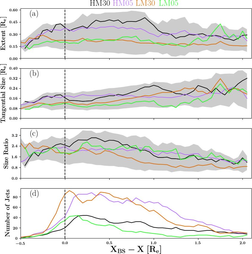
294                                                                                  M. Palmroth et al.: Magnetosheath jet statistics

Figure 2. Left column: virtual spacecraft. Right column: MMS data from the position indicated by a star in Fig. 1a and b. The position is given
in GSE coordinates in Earth radius (RE ), added above the panels. The positions are close to each other but not identical because the Vlasiator
velocity distributions are not saved everywhere. From top to bottom in both Vlasiator and MMS, we show the dynamic pressure, three
components and the magnitude of the velocity, three components and the magnitude of the magnetic field, the ion energy–time spectrogram,
density, and temperature.

Nevertheless, we adopt an inclusive strategy and include all              cur in many statistical data sets. Further, based on Movie S1
events fulfilling the jet criterion. This is to increase similar-         we also limit our study to smaller jets and avoid large re-
ity to the observational statistics, as none of the statistical           gions near flanks because we suspect that the jet criterion
studies of jets using spacecraft measurements have an op-                 may falsely identify regions where the flow becomes super-
portunity to confirm the place of their origin or whether the             Alfvénic as jets.
magnetosheath flow conditions altered due to, for example,                   Applying the jet criterion and the other restrictions de-
kinetic-mode waves such that the local parameters fulfil the              scribed above to the identification routine, we found a to-
jet criteria. Based on Movie S1, we suspect that this may oc-             tal of 924 jets from the four runs, whose xy GSE positions

Ann. Geophys., 39, 289–308, 2021                                                            https://doi.org/10.5194/angeo-39-289-2021
M. Palmroth et al.: Magnetosheath jet statistics                                                                                        295

                                                                        Table 2. Jets in the four runs listed in Table 1. The first (second)
                                                                        column is the start (stop) time of the simulation when the jet search
                                                                        began (ended). The third column gives the number of jets found in
                                                                        each run.

                                                                                                Jet search    Jet search   Number
                                                                                                  start [s]     stop [s]    of jets
                                                                                 Run HM30             290         419.5        144
                                                                                 Run HM05             290         589.5        293
                                                                                 Run LM30             290         669.5        368
                                                                                 Run LM05             290         439.5        119

                                                                        of the magnetic field rotation angle 15 min before and 5 min
                                                                        after the jet is smaller than 45◦ . As a result, the MMS data
                                                                        set contains 6142 jets from the beginning of mission data to
                                                                        the end of May 2019. This set is further divided into low
Figure 3. Jets position in the xy plane in the GSE coordinate sys-      and high MA (MA < 6, and MA > 6, respectively), resulting
tem. The jets identified in the four Vlasiator runs described in Ta-    in 577 and 5533 jets, respectively. Figure 3 shows the high
ble 1 are shown as purple (orange) dots, which represent low (high)     (low) MA jets found from the MMS data as purple (light
MA from runs LM30 and LM05 (HM30 and HM05), respectively.               blue) crosses.
The total number of jets is 924. Only one position during their life-
time is depicted; this is when the jet was at its largest extent. The   4.2   Statistical properties of the jets: Vlasiator and
purple and light blue crosses give the position of the high and low           MMS results
MA MMS jets, respectively. A total of 6142 jets are found from the
MMS data. The number of low and high MA categories is 577 and
                                                                        Before we present the statistical properties of the Vlasiator
5533, respectively, for the MMS, using the same MA criterion as for
Vlasiator. The approximate magnetopause and bow shock positions
                                                                        and MMS jets, we summarise the differences of the obser-
are given by solid black lines.                                         vation criteria in Vlasiator and in MMS. Figure 4 illustrates
                                                                        the lifetime evolution of an imaginary jet starting at the bow
                                                                        shock (marked as BS in Fig. 4) and ending up near the mag-
                                                                        netopause (MP). The black line delineates the jet at five dif-
are visible in Fig. 3 as purple and orange dots, representing           ferent times of its life on its journey from the bow shock to
low and high MA runs, respectively. The number of jets in               the magnetopause. The red dot represents the geometric cen-
the different runs is also presented in Table 2. Since the runs         tre position of the jet. In the following statistical data set, the
are carried out with different solar wind conditions, the po-           Vlasiator jets can be depicted at any time during their life,
sition of the magnetopause and bow shock is not the same                and their properties can be obtained at a given time or as a
between the runs, and therefore the average positions of the            function of the jet lifetime. In contrast, the MMS crosses the
magnetopause (Shue et al., 1998) and the bow shock (Merka               jet at a random time at a random position. To facilitate the
et al., 2005) do not represent the reality for an individual jet        comparison between Vlasiator and MMS, in the following
observation. The jets appear at different distances along the           statistics we present the Vlasiator data in two different man-
x axis in each run, reflecting the solar wind conditions and            ners. First, we describe the Vlasiator jet properties at time
the consequent magnetosheath position in each run. They are             “VLMax”, i.e. at the time when the jet is at its largest size,
evenly distributed in terms of their y position within the mag-         and at the position where the parameter has its maximum
netosheath. The largest number of jets is found in run LM30,            value within the jet (see Fig. 4). However, as it is not known
which has the lowest MA and a 30◦ IMF cone angle. This run              whether the MMS crosses the jet when it is at its largest
was carried out longer than the other runs, indicating that run         size, or where the crossing takes place within the jet, we also
LM30 is overemphasised in the statistical results.                      present the Vlasiator data at a time “VLRand”, i.e. at the po-
   The MMS data set consists of jets fulfilling the Archer cri-         sition where the parameter is at its maximum, at a random
terion using the 20 min averaging. To facilitate comparison             time of the jet evolution. This manner is adopted for other
with Vlasiator, we impose a stability criterion on the solar            parameters except for temperatures, which are averaged from
wind. This is to increase confidence that the jets included in          within the jet, not taken at the maximum value due to a large
the statistics contain stable solar wind conditions and, there-         variation of the temperature. Figure 4 also presents the MMS
fore, can be meaningfully compared with Vlasiator results,              crossing of the jet in blue, taking place at a random position
which are obtained with synthetic stable solar wind. This sta-          through the jet at a random time during the jet lifetime. Fur-
bility criterion requires that the maximum standard deviation           ther, since our run set does not represent all solar wind values

https://doi.org/10.5194/angeo-39-289-2021                                                           Ann. Geophys., 39, 289–308, 2021
296 M. Palmroth et al.: Magnetosheath jet statistics
ment, and the median values are in quantitative agreement.
The maximum magnetic field shows a narrower distribution
in Vlasiator as compared to the distribution using the MMS
data, and the MMS jets are also more intense in terms of the
magnetic field (the median value of the maximum magnetic
field inside the jet is 6.2 times larger than the IMF, while in
Vlasiator at random times it is about 3.1 times larger than
the IMF). The last row shows the temperature distributions
of the jets. The Vlasiator jets are about 3 times hotter than in
the MMS observations both in the parallel and in the perpen-
Figure 4. Illustration of the differences in detecting jets from Vlasi- dicular direction. There is also a separation in the Vlasiator
ator and from MMS data (see text for details). The Vlasiator statis- jets, such that the perpendicular temperature is larger than the
tical data are given at two different times: the time of the maximum parallel temperature. The MMS distribution shows no such
size of the jet (“VLMax”) and at a random time (“VLRand”). In separation, and the median temperature in both the parallel
both cases the data are retrieved from the position of the largest and perpendicular direction is about 3 MK.
value, except for temperatures. Temperatures are averaged over all Figure 6 shows a similar histogram setup as in Fig. 5. In-
positions within the jet. The time or place of the MMS jet cross-
stead of the value within the jet, we now present a histogram
ing is not known relative to the jet lifetime; therefore MMS data
made by subtracting the ambient magnetosheath value from
are given when MMS is observing the jet, i.e. at time “MMS Max”,
illustrated in blue. the jet value. To do this, we define a thin shell of two simu-
lation cells outside the jet area, take the average of this shell,
and subtract it from the jet maximum value. For tempera-
ture (the first row showing a histogram of 1T ), we subtract
detected in the MMS observational data set, we make the sta- the shell average temperature from the average temperature
tistical comparison with respect to the solar wind in the fol- within the jet. The normalised histograms are also separated
lowing manner. First, in Figs. 5 and 6 we use normalisation to such that the blue (red) colour indicates jets during low (high)
the solar wind values as units both in the Vlasiator and in the MA in the solar wind. The threshold between high and low
MMS data. Second, in Fig. 6 we show the results using values MA is 6 in both Vlasiator and MMS. Figure 6 again shows
from which the background has been subtracted. While vari- an excellent agreement between Vlasiator and MMS data,
ation in the observations will certainly depend on the solar both in terms of distribution shapes and quantitatively. Over-
wind conditions, by subtracting the background conditions all, no large differences appear between the low and high
and normalising to the solar wind, we minimise this effect. MA distributions other than in the magnetic field intensity.
Figure 5 presents the statistical properties of the Vlasia- In the last row of Fig. 6, we note that during high MA , the
tor and MMS jets. The first two columns refer to Vlasiator magnetic field intensity differences between the jet and the
times VLMax and VLRand as illustrated in Fig. 4, while the magnetosheath are consistently larger, both in Vlasiator and
third column gives the MMS jet statistics. From top to bot- in MMS. In other words, during high MA , the jet magnetic
tom, each row depicts a histogram of the jet extent, density, field increases relative to the magnetic field within the mag-
speed, dynamic pressure, magnetic field magnitude, and tem- netosheath, as compared to jets during low MA .
perature, respectively. The parameter “extent” in Vlasiator is
the size of the jet in RE in the x direction, and it is com-
pared to the distance which the MMS traverses within the 5 Jet properties: Vlasiator results
jet as determined by the identifying criterion. All other pa-
rameters except the extent and temperature are normalised According to Figs. 5 and 6, the Vlasiator jet statistics are in
to the respective solar wind values. Taking into account that good quantitative correspondence with the MMS statistics.
the simulation results represent four solar wind conditions, Therefore we next present Vlasiator results of jet characteris-
while the MMS data are gathered during a larger variety of tics using the power of the modelling tool describing, for ex-
conditions, Fig. 5 shows an overall agreement, especially be- ample, the time evolution of the jet. Figure 7 shows Vlasiator
tween the Vlasiator jets at random times and the MMS jets. histograms of the jet lifetime, tangential size (at its largest),
Possibly due to the discrepancy in determining the jet extent, and size ratio, defined as the jet radial size divided by the
the MMS jets appear slightly larger than the Vlasiator jets, tangential size at the time when the jets are at their largest
and they span a broader range of scales. The second row de- extent. The radial size is computed as the difference of the
scribes the maximum density inside the jets, indicating that maximum and minimum points of the jet in the radial direc-
the median density of the Vlasiator (MMS) jets at random tion from the centre of the Earth. The tangential size is the
times is 4.9 (5.9) times the solar wind density. The shapes of jet total area divided by the radial size. All histograms show
the Vlasiator and MMS jet maximum velocity and maximum the normalised number of jets. Figure 7a shows that most of
dynamic pressure distributions are in good general agree- the jets in all runs are short-lived, with a median lifetime of
Ann. Geophys., 39, 289–308, 2021 https://doi.org/10.5194/angeo-39-289-2021M. Palmroth et al.: Magnetosheath jet statistics 297 Figure 5. Histograms of Vlasiator (two first columns) and MMS jets (third column) at times and positions specified in Fig. 4. From top to bottom we present histograms of the jet total extent, maximum density, maximum velocity, maximum dynamic pressure, maximum magnetic field intensity, and maximum temperature. The extent is given in Earth radii and the temperature in megakelvins; however, all other parameters are given as normalised to the respective solar wind and IMF values. The bottom row gives both the parallel and perpendicular temperatures in blue and black, respectively. The top right corner of each panel gives the median and standard deviation of the respective histogram. https://doi.org/10.5194/angeo-39-289-2021 Ann. Geophys., 39, 289–308, 2021
298                                                                                   M. Palmroth et al.: Magnetosheath jet statistics

Figure 6. Histograms of Vlasiator and MMS jets in a similar setup as in Fig. 5. Now, the histograms present a difference between the value
within the jet and the value outside the jet. From top to bottom we present the difference of the jet and magnetosheath temperature, density,
velocity, dynamic pressure, and magnetic field intensity, all again normalised to the solar wind values. Red (blue) indicates the data set having
higher (lower) MA .

less than 11 s. However, in all runs there are jets which can              tio, as a function of the jet position relative to the bow shock.
last over 50 s. Interestingly, there is a larger share of short-           The bow shock position is defined to be where the heating of
lived jets during low MA (green and orange histograms in                   the core population is larger than 3 times the solar wind tem-
Fig. 7a) than during high MA . The tangential size (Fig. 7b) is            perature, similarly as in Battarbee et al. (2020). The epoch
around 0.1 RE in all runs, with little variability between the             x axis is defined from the difference of the bow shock and jet
driving conditions. The size ratio (Fig. 7c) is mostly slightly            x coordinates, indicating that 0 means bow shock, and larger
larger than 1, indicating jets of ∼ 0.1 by 0.1 RE , with the ra-           numbers indicate deeper regions towards the magnetopause.
dial size perhaps slightly larger. Again, only small variability           The zero epoch position is chosen when the jet is at the bow
is detected in the size ratio histograms between runs.                     shock. Figure 8 shows that some jets appear upstream before
   Figure 8 presents a modified superposed epoch study of                  the 0 epoch position. This is because jets are identified up
the Vlasiator jets in all runs. By “modified”, we mean that                to 0.5 RE sunward of the polynomially fitted bow shock so
we do not use time in the epoch axis but convert the time se-              as not to exclude jets in regions where the shock is locally
ries at the centre of the jet to a position profile given at the           sunward of the fit. The different colours give the modified
x axis. Depicted are the jet extent, tangential size, and size ra-         superposed epoch average for the different runs, with green

Ann. Geophys., 39, 289–308, 2021                                                             https://doi.org/10.5194/angeo-39-289-2021
M. Palmroth et al.: Magnetosheath jet statistics                                                                                                   299

Figure 7. Histograms of Vlasiator jets illustrating (a) the jet lifetime, (b) the jet tangential size, and (c) the jet size ratio, defined as the radial
size divided by the tangential size. The colours refer to the different runs, with the run identifier (see Table 1): orange and green (black and
purple) are the low (high) MA runs, respectively.

Figure 8. Superposed epoch study of the (a) extent, (b) tangential size, (c) size ratio (defined as in Fig. 7c), and (d) number of jets as a
function of the jet average centre position (red dot in Fig. 1a and b) relative to the bow shock. The different colours refer to the superposed
epoch averages from the different runs, identified with a run identifier (see Table 1): orange and green (black and purple) are the low (high)
MA runs, respectively. Grey shows standard deviations subtracted and added to the average, taken from all jets.

https://doi.org/10.5194/angeo-39-289-2021                                                                   Ann. Geophys., 39, 289–308, 2021
300                                                                           M. Palmroth et al.: Magnetosheath jet statistics

and orange (purple and black) representing the low (high)           dividual jet shows interesting features that are smeared out
MA runs, respectively. Grey shows standard deviations sub-          in the overall statistics. The jet density increases fast after
tracted and added to the average, taken from all jets.              the bow shock, indicating initial compression. The dynamic
   Figure 8 shows a consistent difference between the high          pressure and magnetic field intensity show also a stronger
and low MA runs, as in the high MA runs the jets show a             increase after the bow shock, suggesting compressive be-
larger extent and a larger tangential size as compared to the       haviour. Towards the end of its lifetime, the density, veloc-
low MA runs. The size ratio is smallest for run LM30 (which         ity, dynamic pressure, and magnetic field intensity generally
has a 30◦ IMF cone angle with low MA ), while for the other         decrease. Both temperatures are cooler than the surround-
runs the size ratio does not change much according to the           ings when the jet was born, while the structure thermalises
driving conditions. Although in Fig. 7c the size ratio median       towards the end of its life. Based on Fig. 10 the jet ceases
is slightly larger than 1, according to Fig. 8c, the size ra-       to exist through diffusion rather than disintegration because
tio can be over 2 at maximum, indicating that the radial size       towards the end of its lifetime there are no steep gradients
prevails. A clear feature shown in Fig. 8b and c is that jets are   within the jet parameters (without counting the final sec-
flattening as they propagate deeper into the magnetosheath:         onds).
the tangential size increases and the size ratio decreases from        Next, we investigate how the jet moves through the mag-
the bow shock towards the magnetopause. To verify this be-          netosheath relative to the overall flow, again a feature that
haviour, we identified a particularly strong jet and followed       can only be studied using a global model. Figure 11 shows
its size parameters from the bow shock to come to this same         the jet velocity deflection away from the Sun–Earth line rel-
conclusion (not shown).                                             ative to the background magnetosheath flow. The plot con-
   Figure 9 shows a similar superposed epoch study as a func-       struction is similar to Figs. 8–9 as a modified superposed
tion of the jet position relative to the bow shock as in Fig. 8;    epoch is presented, and the epoch x axis is defined from
however, now we present the difference between the jet and          the difference of the bow shock and jet x coordinates. Fig-
the surrounding magnetosheath environment. For example,             ure 11a shows the magnitude of the velocity deflection rela-
panel (a) presents the difference in density, calculated by         tive to the background,
                                                                                    q         and it is constructed in the following
subtracting the average magnetosheath density (in a two-cell        manner: |v| = vx2 + vy2 , where vx and vy are the compo-
shell around the jet) from the maximum density value inside
                                                                    nents of the jet velocity in the x and y directions, respec-
the jet. Therefore, each epoch curve represents how much the
                                                                    tively. The magnetosheath velocity h|v|i is the average mag-
jet value increases or decreases from the neighbouring mag-
                                                                    netosheath velocity at each respective jet position during the
netosheath as a function of position from the bow shock. Fig-
                                                                    duration of the run. In effect, this average magnetosheath ve-
ure 9 shows again consistently that the jets during high solar
                                                                    locity thus represents the average flow of the magnetosheath
wind MA are denser and faster, and they have a more intense
                                                                    within the position where the jet is at any given time during
dynamic pressure and magnetic field relative to the surround-
                                                                    its progression within the magnetosheath. Figure 11a shows
ing magnetosheath, compared to the jets during low MA . The
                                                                    that for all other runs except run LM30, |v| − h|v|i is posi-
density, velocity, dynamic pressure, and magnetic field inten-
                                                                    tive, indicating that the jet progresses faster than the back-
sity epoch curves all behave similarly: after the bow shock
                                                                    ground magnetosheath flow and that during the progression
these parameters show an initial maximum first, and towards
                                                                    towards the magnetosheath, the jet velocity slows down to-
the magnetopause they decrease from the maximum. The
                                                                    wards the magnetosheath average. For run LM30, curiously,
density, velocity, dynamic pressure, and magnetic field in-
                                                                    the jets progress faster than the magnetosheath flow near the
tensity are positive all the way, indicating that the jet itself
                                                                    bow shock, but then |v| − h|v|i becomes negative on average,
shows larger values than those within the magnetosheath.
                                                                    meaning that the jets travel slower compared to the magne-
The temperatures behave differently, as in the vicinity of the
                                                                    tosheath when they get further from the bow shock.
shock the temperature differences are generally lower and
                                                                       Figure 11b shows the deflection angle, where θ =
negative and increase towards the magnetopause. This means
                                                                    arctan(|vy |/−vx ) is the deflection angle away from the Sun–
that the jets start cooler than the surrounding magnetosheath
                                                                    Earth line, and hθ i is the average of the deflection angle
and thermalise as they progress through the magnetosheath.
                                                                    of the magnetosheath within the position where the jet is
Overall, there is considerably more variation in the tempera-
                                                                    at any given time during its progression within the magne-
ture. The 30◦ cone angle run with high Mach number (black
                                                                    tosheath throughout the run. Therefore Fig. 11b illustrates
curve) shows the coolest values within the jet relative to the
                                                                    how much on average the jet velocity is deflected from the
surrounding magnetosheath.
                                                                    Sun–Earth line relative to the background flow pattern. Fig-
   To show how an individual, particularly strong jet behaves
                                                                    ure 11b shows that for all other runs except run LM30, the
in time, we show in Fig. 10 one jet identified from run HM05
                                                                    deflection angle is negative, indicating that the jets on av-
(purple curves in Figs. 7–9) as a function of the simulation
                                                                    erage travel more along the Sun–Earth line than along the
time rather than position from the bow shock. The properties
                                                                    magnetosheath flow. In other words, the average flow pattern
are taken from the centre of the jet at each time step. The
                                                                    within the jet position is more towards the flanks relative to
general behaviour is the same as in Fig. 9; however, the in-

Ann. Geophys., 39, 289–308, 2021                                                    https://doi.org/10.5194/angeo-39-289-2021
M. Palmroth et al.: Magnetosheath jet statistics 301
Figure 9. Superposed epoch study of the difference between the jet and magnetosheath (a) density, (b) velocity, (c) dynamic pressure,
(d) magnetic field intensity, (e) perpendicular temperature, and (f) parallel temperature as a function of jet position relative to the bow shock.
All other parameters are normalised to the solar wind, while the temperature data are given in megakelvins. The different colours refer to the
superposed epoch averages from the different runs, identified with a run identifier (see Table 1): orange and green (black and purple) are the
low (high) MA runs, respectively. Grey shows standard deviations subtracted and added to the average, taken from all jets.
the jet flow direction. However, in run LM30, θ − hθi is pos- to the side of the magnetosheath, which is behind the quasi-
itive, indicating that these structures flow more towards the parallel bow shock. This same tendency can also be seen in
flanks than the average flow direction with the jet position. the almost radial runs, while it is slightly smaller in magni-
Finally, in Fig. 12 we investigate where the jets end up tude.
within the magnetosheath. Figure 12a shows the jet end co-
ordinate in y, while Fig. 12b shows the jet end angle in the
xy plane, and black (purple) lines give the results for the 30◦ 6 Discussion and conclusions
(5◦ ) cone angle, grouping both the low and high solar wind
MA runs. Figure 12 thus illustrates the difference in event oc- In this paper we have rigorously compared magnetosheath
currence patterns regarding location behind the quasi-parallel jets identified from the Vlasiator simulation in four runs
and quasi-perpendicular bow shock. Figure 12 clearly shows with jets identified from MMS observations. We confirm that
that the jets tend to end up in the dawn flank of the magne- the Vlasiator jet properties are statistically in an excellent
tosheath especially during the 30◦ cone angle runs, that is, quantitative agreement with the observational MMS statis-
tics. Further, we note that individual jets from Vlasiator and
https://doi.org/10.5194/angeo-39-289-2021 Ann. Geophys., 39, 289–308, 2021302 M. Palmroth et al.: Magnetosheath jet statistics Figure 10. The difference between the jet and magnetosheath (a) density, (b) velocity, (c) dynamic pressure, (d) magnetic field intensity, (e) perpendicular temperature, and (f) parallel temperature as a function of jet lifetime in the simulation for a chosen particularly strong jet in run HM05 (purple curves in Figs. 7–9). All other parameters are normalised to the solar wind, while the temperature data are given in megakelvins. MMS suggest quantitative agreement in the dynamic pres- magnetosheath-like. In addition, we find that the largest de- sure, even though the jets are identified during different so- viations from the ambient magnetosheath values occur just lar wind conditions. After noting the quantitative agreement, after the bow shock, while towards the magnetopause the pa- we show Vlasiator results of the statistical behaviour of the rameters start to approach the magnetosheath values. The jets jets as a function of lifetime and relative position from the appear first compressive and cooler than the magnetosheath, bow shock. We find that overall, Vlasiator jets during low while during their propagation they thermalise. The jets are solar wind MA are shorter in duration and smaller in their able to maintain their flow through the magnetosheath, and extent as compared to the jets during high MA . The shape of they preferentially end up to the side of the magnetosheath, the jets changes as they progress through the magnetosheath. which is behind the quasi-parallel shock. Further, we confirm the findings of Plaschke et al. (2013) Two assumptions have been made in Vlasiator to reach in that the jets are faster and denser and have a higher dy- these conclusions about magnetosheath jets; i.e. we carry out namic pressure and more intense magnetic field as com- the simulations in two spatial dimensions (2D) and assume pared to the ambient magnetosheath near the bow shock. that electrons are a massless charge-neutralising fluid. Both They are also cooler relative to the magnetosheath. Towards simplifications are made due to huge computational demands the magnetopause, the jet characteristics start to be more that are already in place with the 2D3V approach that re- Ann. Geophys., 39, 289–308, 2021 https://doi.org/10.5194/angeo-39-289-2021
M. Palmroth et al.: Magnetosheath jet statistics                                                                                              303

Figure 11. Jet velocity deflection away from the Sun–Earth line relative to the background magnetosheath velocity, in terms of (a) magnitude
of velocity deflection and (b) angle of the velocity deflection. See text for details on the definition of the depicted parameters. The grey lines
indicate all events, while different colours refer to the superposed epoch averages from the different runs, identified with a run identifier (see
Table 1): orange and green (black and purple) are the low (high) MA runs, respectively.

Figure 12. Jet end position within the magnetosheath in terms of (a) the y coordinate and (b) 8 = arctan(y/x), where [x, y] are the last
coordinates of the jet when it was still detected. The black line gives the jets for the runs with a 30◦ cone angle, while the purple lines are the
results for the 5◦ cone angle.

https://doi.org/10.5194/angeo-39-289-2021                                                                Ann. Geophys., 39, 289–308, 2021
304                                                                            M. Palmroth et al.: Magnetosheath jet statistics

quires a supercomputer with a large runtime memory. In fact,         find that the perpendicular (parallel) size is between 0.2 and
no 3D global kinetic or hybrid-kinetic simulations of jets cur-      0.5 RE (1 RE ), while we, using the same criterion, find that
rently exist to which these results could be compared to. The        the mean tangential size is about 0.1 RE and that the radial
bow shock–magnetosheath interactions are rather accurately           size is dominating over the tangential size. Plaschke et al.
reproduced by 2D kinetic simulations as can be seen from the         (2016) find that the sizes are 1.34 RE and 0.71 RE in perpen-
spacecraft comparison shown in this paper and from a large           dicular and parallel direction, respectively, while Plaschke
number of previous papers (e.g. Blanco-Cano et al., 2006;            et al. (2020) report scale sizes of 0.12 RE and 0.15 RE . Our
Karimabadi et al., 2014). The largest caveat of the 2D3V ap-         results are hence in excellent agreement with the reported lit-
proach is that the position of the magnetopause is difficult to      erature, regardless of the identification criteria.
determine, which is why we avoid making conclusions near                The evolution of the jet size is very difficult to investigate
the magnetopause.                                                    using spacecraft observations, and therefore to the best of our
   As for neglecting the electron dynamics in a hybrid               knowledge our results give the first estimations on how the
scheme, first we note that the kinetic pressure of the elec-         jets evolve as they progress through the magnetosheath. Our
trons downstream of the Earth’s bow shock is smaller by              results show that the jet shape seems to be flattening, and the
about a factor of 10 with respect to the ion pressure. The           tangential size increases while the size ratio decreases from
fact that the observational jet dimensions are between fluid         the bow shock towards the magnetopause. The size ratio de-
and ion-kinetic scales indicates that an ion-kinetic model ne-       creases for all runs, and especially so in run LM30, which is
glecting kinetic electrons should be sufficient to investigate       the run with the lowest MA . In this run (given with the or-
jet sizes. To understand the electromagnetic effects due to the      ange line in Fig. 8) the jets seem to flatten within the first RE
absence of kinetic electrons, one must consult kinetic simu-         within the magnetosheath, while for other runs the flatten-
lations including both ions and electrons, which on the other        ing occurs further downstream. Figure 9c indicates that the
hand have to limit the simulation volumes due to computa-            dynamic pressure and magnetic field intensity for the LM30
tional restrictions. Voitcu and Echim (2016, 2018) investigate       run jets are smallest compared to the other runs throughout
the propagation of jet-like features through a plasma having a       their journey from the bow shock towards the magnetopause.
transverse magnetic field. They find that a polarisation elec-       Hence, the rapid flattening of the LM30 jets, together with
tric field forms inside the jet-like feature, contributing to the    the fact that they do not maintain their velocity against the
forward propagation of the jet-like feature across the trans-        magnetosheath flow, is consistent with the notion that these
verse background magnetic field. This process is neglected in        jets appear to be “weakest” in the statistics, and they slow
our simulation in the absence of kinetic electrons. It is diffi-     down most rapidly in the magnetosheath. This suggests that
cult to speculate what the additional polarisation electric field    the strength of the jets is related to the strength of the shock.
would cause in our simulations, especially as our simulations           Continuing with the differences organised by the MA , we
do not have a transverse background magnetic field but are           find that the extent of the jet, giving the jet instantaneous size
carried out during a solar wind cone angle ranging from ra-          in the x direction, is larger for the high MA runs as compared
dial to Parker spiral conditions. In the radial runs (HM05 and       to the low MA runs. The jets associated with low MA are also
LM05) the magnetic field is highly turbulent at the subso-           shorter in duration as compared to the jets during high MA .
lar magnetosheath, and in the HM30 and LM30 runs it is               This interesting feature may be related to the nature of the
a bit less turbulent but definitely not purely transverse (not       foreshock during the different conditions. Turc et al. (2019)
shown). Therefore this effect could be studied perhaps us-           demonstrated that the foreshock wave field is different dur-
ing the new eVlasiator (Battarbee et al., 2021) with electron        ing different MA and that for low MA the wavelengths and
capabilities to investigate this aspect in the future.               the transverse extents of the foreshock monochromatic waves
   According to Plaschke et al. (2016), the jet scale sizes may      were much smaller as compared to foreshock waves during
convey information about how the jets came into existence,           high MA . The characteristics of the foreshock may be related
and therefore it is important to characterise the jet size distri-   to the origin of the jets at least in two ways: first, Burgess
butions. The observational statistics have so far characterised      (1995) suggests that the bow shock ripples are modulated by
the jet sizes in two directions, parallel and perpendicular to       the foreshock waves. Therefore, if the foreshock waves are
the direction of propagation, while Vlasiator results char-          small, the bow shock ripples, suggested to be the origin of
acterise the jets in radial and tangential directions. Another       the jets (Hietala et al., 2009), are also small, and the jet be-
point which influences the direct comparison is that in Vlasi-       comes small. In this scenario, the perpendicular size of the
ator the size is determined as the area delineated by the jet        jet is coupled to the perpendicular scale of the ULF wave,
criterion contour, while in observational statistics it is de-       and the parallel size of the jet is coupled to the parallel wave-
termined essentially from the time that it takes for the jet         length of the foreshock ULF wave. Second, however, it is
to traverse past the spacecraft. Further, to determine the jet       also possible that the smaller foreshock ULF waves during
perpendicular size, multi-spacecraft methods need to be em-          low MA do not steepen to form strong compressional struc-
ployed, and therefore not many statistics can be found where         tures (like SLAMS), which would easily travel through the
both dimensions are estimated. However, Archer et al. (2012)

Ann. Geophys., 39, 289–308, 2021                                                      https://doi.org/10.5194/angeo-39-289-2021
You can also read