Estimation of groundwater recharge from groundwater levels using nonlinear transfer function noise models and comparison to lysimeter data
←
→
Page content transcription
If your browser does not render page correctly, please read the page content below
Hydrol. Earth Syst. Sci., 25, 2931–2949, 2021
https://doi.org/10.5194/hess-25-2931-2021
© Author(s) 2021. This work is distributed under
the Creative Commons Attribution 4.0 License.

Estimation of groundwater recharge from groundwater levels
using nonlinear transfer function noise models
and comparison to lysimeter data
Raoul A. Collenteur1 , Mark Bakker2 , Gernot Klammler3 , and Steffen Birk1
1 Institute
         of Earth Sciences, NAWI Graz Geocenter, University of Graz, Heinrichstrasse 26, 8010 Graz, Austria
2 WaterManagement Department, Faculty of Civil Engineering and Geosciences, Delft University of Technology,
Stevinweg 1, 2628 CN, Delft, the Netherlands
3 JR-AquaConSol GMHB, Graz, Austria

Correspondence: Raoul A. Collenteur (raoul.collenteur@uni-graz.at)

Received: 30 July 2020 – Discussion started: 27 August 2020
Revised: 18 February 2021 – Accepted: 25 April 2021 – Published: 31 May 2021

Abstract. The estimation of groundwater recharge is of              extended to support applications in different hydrogeologi-
paramount importance to assess the sustainability of ground-        cal settings than those presented here.
water use in aquifers around the world. Estimation of the
recharge flux, however, remains notoriously difficult. In
this study the application of nonlinear transfer function
noise (TFN) models using impulse response functions is ex-          1   Introduction
plored to simulate groundwater levels and estimate ground-
water recharge. A nonlinear root zone model that simulates          Despite ongoing scientific efforts, the estimation of ground-
recharge is developed and implemented in a TFN model and            water recharge remains a notoriously difficult task for hy-
is compared to a more commonly used linear recharge model.          drologists (e.g., Bakker et al., 2013). From the many tech-
An additional novel aspect of this study is the use of an           niques available (see, e.g., Healy and Scanlon, 2010, for
autoregressive–moving-average noise model so that the re-           an overview), methods using groundwater-level observations
maining noise fulfills the statistical conditions to reliably es-   as the primary source of information are among the most
timate parameter uncertainties and compute the confidence           popular. This is likely due to the abundance of available
intervals of the recharge estimates. The models are calibrated      groundwater-level data and the simplicity of the methods
on groundwater-level data observed at the Wagna hydro-              (Healy and Cook, 2002). A well-known example is the wa-
logical research station in the southeastern part of Austria.       ter table fluctuation (WTF) method, which only requires an
The nonlinear model improves the simulation of groundwa-            estimate of the specific yield and groundwater-level data as
ter levels compared to the linear model. The annual recharge        model input. An additional advantage of the WTF method
rates estimated with the nonlinear model are comparable             is that no assumptions are made about the actual recharge
to the average seepage rates observed with two lysimeters.          processes, for example, the existence of preferential flow
The recharges estimates from the nonlinear model are also           paths. This can also be considered a disadvantage, as no re-
in reasonably good agreement with the lysimeter data at             lationship between precipitation and recharge is established.
the smaller timescale of recharge per 10 d. This is an im-          This makes the method unsuitable for future projections of
provement over previous studies that used comparable meth-          groundwater recharge when precipitation patterns change,
ods but only reported annual recharge rates. The presented          for example, in climate change impact studies.
framework requires limited input data (precipitation, poten-           In a review paper on the topic, Healy and Cook (2002)
tial evaporation, and groundwater levels) and can easily be         suggested that “approaches based on transfer function noise
                                                                    (TFN) models should be further explored” for the estima-

Published by Copernicus Publications on behalf of the European Geosciences Union.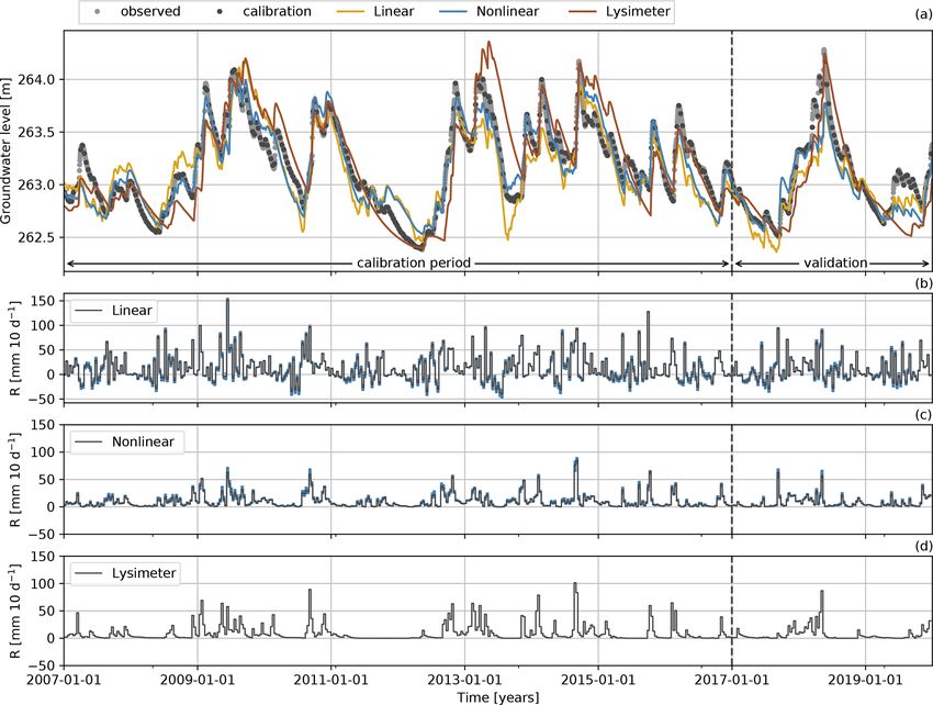
2932               R. A. Collenteur et al.: Estimating groundwater recharge from groundwater levels using TFN models

tion of recharge. TFN models can be used to translate one             More recently, efforts have been made to explore the
or more input series (e.g., precipitation and potential evap-      use of TFN models to estimate groundwater recharge, as
oration) into an output series (e.g., groundwater levels) and      suggested by Healy and Cook (2002). Hocking and Kelly
have been adopted in many branches of hydrology (Hipel and         (2016) constructed TFN models that included rainfall, evap-
McLeod, 1994). An early example of the use of these models         oration, river levels, pumping, and a linear trend as ex-
for recharge estimation is given in Besbes and De Marsily          planatory variables, to isolate the contribution of rainfall
(1984), through the deconvolution of groundwater levels            to the groundwater-level fluctuations. This contribution was
with an aquifer unit hydrograph obtained from a groundwa-          then converted to recharge using the hydrograph fluctuation
ter model. The study showed how the recharge flux can be           method (Viswanathan, 1984). Obergfell et al. (2019) used a
related to rainfall by using an additional unit hydrograph for     linear model to estimate average diffuse recharge and ob-
the unsaturated zone. Their proposed method required a cali-       tained good annual recharge estimates when compared to re-
brated groundwater model and a good estimate of the infiltra-      sults from a chloride mass balance. Recognizing the impor-
tion, making the method relatively laborious and less applica-     tance of evaporation in their model setup, they constrained
ble in practice. O’Reilly (2004) developed a water balance–        the parameter estimation by including the correct simulation
transfer function model to simulate recharge, using the WTF        of the seasonal behavior in the objective function. Peterson
method to obtain recharge estimates to calibrate the model         and Fulton (2019) used a nonlinear TFN model that includes
parameters.                                                        a soil moisture module to estimate recharge (Peterson and
   In recent decades, the use of a specific type of TFN models     Western, 2014). To obtain reasonable estimates of recharge,
using predefined impulse response functions (von Asmuth            the model was constrained by comparing the modeled evap-
et al., 2002) has gained popularity for the analysis of ground-    oration to the expected actual evaporation obtained using the
water levels. In this data-driven method, impulse response         Budyko curve. All of these studies reported annual recharge
functions are used to describe how groundwater levels re-          rates, but at least the latter method could in principle also be
act to different drivers such as precipitation, evaporation, and   used to obtain estimates at smaller timescales.
pumping. The method has been successfully applied to char-            In this study, exploration of the use of nonlinear TFN mod-
acterize and analyze groundwater systems around the world,         els using impulse response functions is continued to estimate
for example in Brazil (Manzione et al., 2010), Italy (Fab-         groundwater recharge and improve the simulation of ground-
bri et al., 2011), the United Kingdom (Ascott et al., 2017),       water levels. A nonlinear recharge model is developed based
and India (van Dijk et al., 2019). The advantages of data-         on a soil-water storage approach and implemented in a TFN
driven models compared to numerical groundwater models             model to simulate the (nonlinear) effect of precipitation and
are faster model development and a lower number of cali-           evaporation on the groundwater levels. This study focuses on
bration parameters (e.g., Bakker and Schaars, 2019). A large       the estimation of recharge for relatively shallow groundwa-
number of time series may be analyzed in a timely manner,          ter systems without capillary rise of groundwater to the un-
for example, to improve the understanding of a groundwater         saturated zone. The estimated recharge fluxes are compared
system. Results are often also useful for the development of       to long-term recharge rates measured with two lysimeters
numerical groundwater models.                                      located at the hydrological research site Wagna in Austria,
   An important goal for these models has traditionally been       providing a unique opportunity to evaluate the recharge es-
to accurately describe observed groundwater-level fluctua-         timates at smaller timescales. Additionally, this study doc-
tions. For shallow water tables (up to a few meters’ depth),       uments the extension of the commonly used autoregressive
this can often be achieved using a linear model between pre-       model with a moving-average part to model the residuals and
cipitation and evaporation on the one hand and groundwa-           obtain an approximately white noise series used for model
ter levels on the other hand; i.e., when the rainfall doubles,     calibration. The purpose of this study is to provide a proof-
so does the increase in the groundwater levels (e.g., Beren-       of-concept of the proposed methods through a detailed case
drecht et al., 2003; von Asmuth et al., 2008). In a large-scale    study for a single location. The data from the lysimeters are
case study for the Netherlands, Zaadnoordijk et al. (2019) ob-     only used to evaluate the model results and are not used to
tained good results with this method for areas with shallow        improve the results during model setup and calibration.
groundwater depths. For the simulation of deeper groundwa-            The next section provides an overview of the study site
ter levels, the linear model was shown to be less appropriate,     and the data used for model input and evaluation. In the third
and nonlinear models may be used to accurately simulate the        section, the methodological approach is described, starting
groundwater levels (e.g., Berendrecht et al., 2006; Peterson       with a brief overview of TFN modeling, followed by a de-
and Western, 2014; Shapoori et al., 2015). Such nonlinear          scription of the recharge models, and ending with a descrip-
models improve the simulation of groundwater levels by tak-        tion of the model calibration. The results are presented and
ing the nonlinear processes that occur in the root zone into       discussed in the fourth section, followed by a general discus-
account, for example, through the limitation of evaporation        sion of the methodology in the fifth section. The conclusions
due to low soil moisture levels and the temporal storage of        of this study are summarized, and recommendations for fu-
water within the root zone.                                        ture research are provided in the sixth and final section.

Hydrol. Earth Syst. Sci., 25, 2931–2949, 2021                                       https://doi.org/10.5194/hess-25-2931-2021
R. A. Collenteur et al.: Estimating groundwater recharge from groundwater levels using TFN models                                  2933

Figure 1. Map of the case study area with the locations of the
lysimeters, the meteorological station, and the groundwater mon-
itoring well used in this study.

                                                                   Figure 2. Time series of the precipitation (P ), potential evaporation
2   Study site and field data                                      (Ep ), recharge (R), and observed groundwater levels (h) for the pe-
                                                                   riod 2006 to 2020. The recharge shown here is the average seepage
The study site is the hydrological research station near the       measured with the two lysimeters.
town of Wagna in Styria, Austria (see Fig. 1). The site is
located in an agricultural field surrounded by residential ar-
eas. Groundwater levels have been observed with a daily time       fall averages only 10 d yr−1 (Prettenthaler et al., 2010). As
step since 1992 (see Fig. 2d; only data from 2006 onwards          the number of days when snowfall occurs is rather limited,
are shown here). The depth to water table is approximately         the effect of snow on groundwater recharge is not taken into
4 m, and no capillary rise of moisture from the water ta-          account in this study.
ble into the root zone is expected due to the existence of a          All the required input time series are measured directly at
coarse gravel layer at a depth of 0.50–120 cm (Klammler and        the site. This includes the precipitation and the meteorolog-
Fank, 2014). The land surface is at 267 m above mean Adri-         ical variables required to calculate potential evaporation. It
atic sea level (a.m.s.l.) with little elevation differences and    is noted here that the term “evaporation” rather than “evapo-
small hydraulic head gradients (±2.5 m km−1 ). The nearest         transpiration” is used throughout this paper (e.g., Savenije,
drainage features are the Sulm River 1 km to the west and          2004; Miralles et al., 2020). The FAO Penman–Monteith
the larger Mur River 1.5 km to the east. Groundwater pump-         method is used to compute the daily grass reference evap-
ing for drinking water purposes occurs 500 m north of the          oration (Allen et al., 1998). Klammler and Fank (2014) and
observation well at a rate of 240 m3 d−1 . Due to the low dis-     Schrader et al. (2013) showed that the estimates from this
charge and high conductivity of the aquifer, the effect of this    method are in good agreement with estimates obtained from
pumping is assumed to be negligible at the study site. Given       a grass lysimeter that is present at the site. The average an-
these conditions, the groundwater-level fluctuations are as-       nual precipitation (P ) and grass reference evaporation (Ep )
sumed to be the exclusive result of changes in the groundwa-       in the period 2007–2019 were 956 and 765 mm yr−1 , respec-
ter recharge from infiltrating precipitation water.                tively. The time series of both fluxes are shown in Fig. 2a and
   The climate at the study area is influenced by the Mediter-     b.
ranean Sea in the south, the land masses of Hungary in the            The study site is equipped with two weighable scientific
east, and the Alps in the west. The average air temperature        field lysimeters, operated by JR-AquaConSol since 2005
is 18.6 ◦ C in summer (June–August) and −0.9 ◦ C in win-           (von Unold and Fank, 2008). The first lysimeter is operated
ter (December–February) (Prettenthaler et al., 2010). In the       under conventional farming practices (Sciencelys 1), while
summer months there are approximately 8 to 9 h sunshine            the second lysimeter (Sciencelys 2) was organically farmed
per day, while during the winter months the number of hours        until 2014, when it was also converted to conventional farm-
with sun averages only 2 to 3 h. Precipitation primarily oc-       ing. A crop-rotation scheme is used for the lysimeters, with
curs as short-duration convective rainfall events during the       crops changing every growing season. The soils in the area
warm summer months. In winter, most of the precipitation           are rather heterogeneous, with the thickness of the sandy
also takes place as rainfall; the number of days with snow-        loamy top layer varying greatly over short distances. The un-

https://doi.org/10.5194/hess-25-2931-2021                                        Hydrol. Earth Syst. Sci., 25, 2931–2949, 2021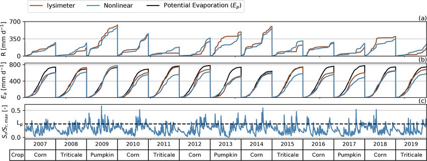
2934               R. A. Collenteur et al.: Estimating groundwater recharge from groundwater levels using TFN models

derlying sand and gravel deposits start at a depth between          ters could not be matched using the Richards equation and a
50–120 cm. Both lysimeters have an area of 1 m2 and are 2 m         Van Genuchten–Mualem approach, suggesting the existence
deep. Seepage to the groundwater is measured near the bot-          of preferential flow paths below the root zone.
tom of the lysimeters at 1.8 m depth, where suction cups are
installed that apply a water potential that is similar to the po-
tential measured with tensiometers just outside the lysime-         3     Methodology
ters. Both lysimeters are identical in their technical setup,
and a detailed description of the lysimeters is provided in         3.1    The basic model setup
von Unold and Fank (2008) and Klammler and Fank (2014).
   As the recharge is not measured at the water table itself,       Transfer function noise (TFN) models are used here to trans-
a certain time lag between the recharge measured with the           late recharge into groundwater levels. The basic model struc-
lysimeters and the corresponding groundwater-level rise ex-         ture is
ists. Only a limited time lag is expected as the ±2 m thick
percolation zone consists mostly of highly conductive gravel
layers. It is noted that the recharge measurements are local        h(t) = hr (t) + d + r(t),                                  (1)
measurements for the area of the lysimeter and are influ-
                                                                    where h(t) [L] are the observed groundwater levels, d [L] is
enced by prevailing soil conditions, vegetation, and the de-
                                                                    the base level of the model, hr (t) [L] is the contribution of
gree of soil sealing. The groundwater levels, measured at ap-
                                                                    the recharge to groundwater-level fluctuations, and r(t) [L]
proximately 12 m distance from the lysimeters at the Wagna
                                                                    are the model residuals. The contribution hr (t) [L] is com-
test site, may also be influenced by different recharge rates
                                                                    puted by convoluting a recharge flux R(t) [L T−1 ] with a pre-
from other land-use types in the surrounding area (e.g., grass-
                                                                    defined impulse response function θ (t) (von Asmuth et al.,
land or residential areas). As such, the measured recharge
                                                                    2002):
rates from the lysimeters are – for the purpose of this pa-
per – used as an indicative rather than an exact estimate of
recharge. Considering the above, the average recharge from                     Zt
the two lysimeters (shown in Fig. 2c) is used in this study for     hr (t) =        R(τ )θ (t − τ )dτ.                         (2)
the comparison with model estimates. The average recharge
                                                                            −∞
measured with the lysimeters is 322 mm yr−1 over the period
2007–2019.                                                             Following Bakker et al. (2008), a four-parameter impulse
   A number of studies have used the hydrological research          response function is used to translate the recharge flux into
site Wagna. Only the literature with a focus on recharge es-        groundwater-level fluctuations:
timation and unsaturated flow modeling is discussed here.
Fank (1999) used the water table fluctuation method to esti-
mate groundwater recharge from observed groundwater lev-            θf (t) = At n−1 e−t/a−ab/t t ≥ 0,                          (3)
els and computed an average recharge of 393 mm yr−1 over
the period 1992–1996. This estimate is comparable to the            where A [T−n+1 ] is a scaling parameter, and a [T], b [–], and
296 and 396 mm yr−1 reported by Stumpp et al. (2009) for            n [–] are shape parameters. For n > 1, the four-parameter
the two lysimeters that were operated at the site in the period     function simulates a delayed response of the groundwater
1992–2001. Stumpp et al. (2009) also applied a HYDRUS-              levels to recharge, while for n ≤ 1 and b = 0, the ground-
1D model to simulate unsaturated zone flow. Using stable            water levels respond instantaneously to a recharge pulse. If
isotope δ 18 O measurements, it was shown that lysimeter            n = 1 and b = 0, Eq. (3) reduces to an exponential response
recharge could be adequately simulated with this physically         function with only two parameters:
based model, although recharge peaks were generally un-
derestimated. Groenendijk et al. (2014) documented a large
comparative study of six different unsaturated zone models,         θe (t) = Ae−t/a t ≥ 0.                                     (4)
where measured water content and fluxes were used to cal-
ibrate and evaluate the models. Although this study focused            The parameters A, a, n, b, and d are estimated by fitting
on nitrate leaching, the study also showed how all models           Eq. (1) to observed data. Depending on the hydrogeological
had difficulties in accurately simulating the water content and     setting and the model used to compute the recharge, either
fluxes observed in the current lysimeters. This was attributed      a four-parameter or an exponential response function is used
to the lack of processes such as hysteresis, preferential flow      here to translate the recharge flux R into groundwater-level
and multiple phase flow in the models. A later study using          fluctuations. The main question that remains is how to esti-
the MIKE SHE model yielded similar results (Reszler and             mate the recharge R(t) from observed hydrometeorological
Fank, 2016). The study concluded that the seepage and water         data. The following two sections introduce the two models
content dynamics in the lower gravel zone inside the lysime-        used in this study to compute the recharge flux R(t).

Hydrol. Earth Syst. Sci., 25, 2931–2949, 2021                                           https://doi.org/10.5194/hess-25-2931-2021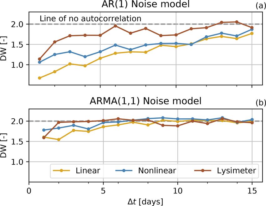
R. A. Collenteur et al.: Estimating groundwater recharge from groundwater levels using TFN models                                 2935

3.2   The linear model

A common approach to approximate the recharge flux R in
Eq. (2) is a simple linear function of precipitation P [L T−1 ]
and potential evaporation Ep [L T−1 ] (e.g., Berendrecht et al.,
2003; von Asmuth et al., 2008):

R = P − f Ep ,                                              (5)

where f [–] is a parameter that is calibrated. The grass ref-
erence evaporation computed using the Penman–Monteith
equation (Allen et al., 1998) is used as potential evapora-
tion Ep here. A clear interpretation of the parameter f is not
available. While Berendrecht et al. (2003) referred to f as        Figure 3. Conceptual model for the nonlinear recharge model.
a crop factor, von Asmuth et al. (2008) noted that the value       Si, max and Sr, max are the maximum capacities of the interception
of f “depends on the soil and land cover” instead of a sin-        and root zone reservoirs, respectively. Ei is the interception evapo-
                                                                   ration, and Et, s is a combined flux consisting of transpiration and
gle crop and also incorporates the “average reduction of the
                                                                   soil evaporation.
evaporation due to actual soil water shortages”. Here, f is re-
ferred to as the evaporation factor, following the terminology
suggested by Obergfell et al. (2019).                              cipitation exceeding the interception capacity continues as
   From Eq. (5), it is clear that the flux R can be negative       effective precipitation (Pe [L T−1 ]) to the root zone reservoir.
for periods when evaporation (f Ep ) exceeds precipitation.        From the root zone, water is evaporated through transpiration
As Eq. (5) does not include a storage term, the temporal dis-      by vegetation and soil evaporation (Et,s [L T−1 ]) or is drained
tribution of recharge that may result from storage in the un-      to become groundwater recharge (R [L T−1 ]). The model is
saturated zone has to be captured by the impulse response          described in more detail below.
function. The four-parameter response function is therefore           To allow the model to adjust the input potential evapo-
used to translate the computed recharge into groundwater-          ration (Ep ) to an evaporation flux that better represents the
level fluctuations for the linear model. As such, the response     vegetation-dependent actual evaporation, a maximum poten-
function simulates the behavior of the entire system: the root     tial evaporation flux Emax [L T−1 ] is computed first:
zone, the unsaturated zone, and the saturated zone. In total,
the linear model has six parameters to be estimated: A, n, a,
and b of the response function (Eq. 3), the evaporation factor     Emax = kv Ep ,                                                   (6)
f , and the base level of the model d (Eq. 1).
                                                                   where kv [–] is a vegetation coefficient that needs to be cal-
3.3   The nonlinear model                                          ibrated. This approach is similar to, for example, the eco-
                                                                   hydrological streamflow model developed by Viola et al.
While the linear model depends on the response function            (2014). The parameter kv is interpreted as a vegetation co-
to simulate the effects of the root zone on the groundwa-          efficient, highlighting the idea that the groundwater recharge
ter recharge, the nonlinear model uses a soil-water storage        may be affected by different types of vegetation instead of a
concept to account for the temporal storage of water in the        single type of crop.
root zone. The nonlinear recharge model developed here is             The water balance for the interception reservoir is
loosely based on the FLEX conceptual modeling framework
used in rainfall-runoff modeling (Fenicia et al., 2006). The       1Si
model is conceptualized as two connecting reservoirs: the              = P − Ei − Pe ,                                              (7)
                                                                   1t
first for interception and the second representing the root
zone, as shown in Fig. 3. Inputs to the nonlinear model            where
are precipitation (P [L T−1 ]) and potential evaporation (Ep
[L T−1 ]).                                                         Ei 1t = min(Emax 1t, Si ),                                       (8)
   The general functioning of the model is as follows. Pre-
cipitation water is intercepted in the first reservoir until the   where Si [L] is the amount of water stored in the intercep-
interception capacity Si,max [L] is exceeded. The intercepted      tion reservoir. The maximum storage capacity of the inter-
water can evaporate from the first reservoir as interception       ception reservoir is determined by the parameter Si, max [L].
evaporation (Ei [L T−1 ]). This process forms the first barrier    Intercepted water is evaporated from the interception reser-
for precipitation to become groundwater recharge (Savenije,        voir, limited by the amount of maximum potential evapora-
2004) and creates a threshold nonlinearity in the model. Pre-      tion Emax (energy-limited) or the amount of water available

https://doi.org/10.5194/hess-25-2931-2021                                        Hydrol. Earth Syst. Sci., 25, 2931–2949, 2021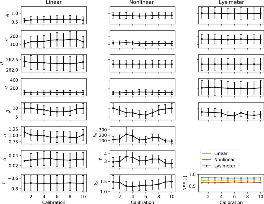
2936                        R. A. Collenteur et al.: Estimating groundwater recharge from groundwater levels using TFN models

for evaporation Si (water-limited). Any precipitation water
exceeding the interception capacity Si, max will continue to
the root zone reservoir as effective precipitation Pe .
   The water balance for the root zone reservoir is

dSr
    = Pe − Et, s − R,                                            (9)
dt
where Sr [L] is the amount of water in the root zone reser-
voir, Et, s [L T−1 ] is a combined evaporation flux constitut-
ing both soil evaporation and transpiration by vegetation,              Figure 4. Relationships between the saturation of the root zone
and R is the recharge to the groundwater. The maximum                   (Sr /Sr, max ) and the fraction of the potential evaporation that is
storage capacity of the root zone reservoir is determined by            evaporated through the root zone (Et, s /Emax ) (a), and the drainage
the parameter Sr, max [L]. The saturation at t = 0 is set to            (R) from the root zone reservoir (b). The saturated hydraulic con-
Sr (t = 0) = 0.5Sr, max . The evaporation flux Et, s is limited         ductivity is set to ks = 1 mm d−1 .
by the amount of water available in the root zone as follows:

                                                                        based on experience and literature values (Savenije, 2010),
                               Sr                                       decreasing the number of parameters that need to be cal-
Et, s = (Emax − Ei )min(1,            ),                        (10)
                           lp Sr, max                                   ibrated. Here, the interception capacity Si, max was set to
                                                                        2 mm, and lp was fixed to 0.25 [–]. The parameter Sr, max was
where the parameter lp [–] determines at what fraction of
                                                                        fixed to 250 mm (e.g., Gao et al., 2014), as it was found to
Sr, max the evaporation flux is limited by the availability of
                                                                        have a strong correlation with ks in the preliminary phase of
soil water. The relationship between the saturation of the root
                                                                        this study and thus hard to calibrate. This leaves a total of
zone (Sr /Sr, max ) and the fraction of the potential evaporation
                                                                        six parameters to be calibrated: kv , ks , and γ of the nonlinear
that is evaporated through the root zone (Et, s /Emax ) is shown
                                                                        recharge model, A and a of the response function (Eq. 4),
in Fig. 4a. It is noted that the maximum potential evapora-
                                                                        and the base level of the model d (Eq. 1).
tion is decreased by the amount of evaporation that already
took place as interception evaporation. The actual evapora-
                                                                        3.4   The Lysimeter model
tion as simulated by the nonlinear model is calculated as
Ea = Et, s + Ei .
                                                                        For comparison, a third model is constructed where the
   Recharge to the groundwater R is computed using Camp-
                                                                        recharge measured with the lysimeters is used as the flux R
bell’s approximation for unsaturated hydraulic conductivity
                                                                        in Eq. (2). Similar to the nonlinear model, an exponential re-
(Campbell, 1974).
                                                                        sponse function is used to translate this recharge into ground-
                                                                        water levels. Assuming that the recharge measured with the
                       γ
                                                                        lysimeters is a good estimate of the (unknown) real recharge,

               Sr
R = ks                      ,                                   (11)    the groundwater levels simulated with this model provide an
             Sr, max
                                                                        indication of the fit that may potentially be obtained with the
where ks [L T−1 ] is the saturated hydraulic conductivity, and          other models.
γ [–] is a parameter that determines how nonlinear this flux is
with respect to the saturation of the unsaturated zone. Equa-           3.5   Noise modeling
tion (11) reduces to the equation used in the FLEX models
(Eq. 4 in Fenicia et al., 2006) when γ = 1 and is similar to            The residuals r(t) of TFN models applied to groundwater-
that used by Peterson and Western (2014). The relationship              level data (see Eq. 1) often show considerable autocorre-
between the saturation of the root zone and the recharge flux           lation. To allow for statistical inferences with the model
for different values of γ is shown in Fig. 4b.                          (e.g., the estimation of confidence intervals of the simulated
   In the preliminary phase of this study, it was found that            recharge), it is necessary to transform the residuals series into
the use of an exponential response function yields similar              a noise series that is approximately white noise. For ground-
results to the four-parameter response function for the non-            water levels time series, this generally means that the auto-
linear model. For reasons of model parsimony, the exponen-              correlation needs to be removed from the residuals. An au-
tial response function (Eq. 4) was adopted for the nonlinear            toregressive model of order 1 (AR(1)) is commonly used for
model to translate the recharge R into groundwater levels.              this purpose (e.g., von Asmuth et al., 2002):
   In total, the nonlinear recharge model has six parameters
that need to be estimated: kv , Si, max , Sr, max , ks , γ , and lp .
Some of these parameters may be fixed to sensible values                υ(ti ) = r(ti ) − r(ti−1 )e−1ti /α ,                            (12)

Hydrol. Earth Syst. Sci., 25, 2931–2949, 2021                                              https://doi.org/10.5194/hess-25-2931-2021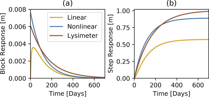
R. A. Collenteur et al.: Estimating groundwater recharge from groundwater levels using TFN models                                   2937

where υ is called the noise series here, 1ti is the time step
between two residuals r(ti ) and r(ti−1 ), and α [T] is the AR
parameter.
   In the preliminary phase of this study, the models were
calibrated using daily groundwater-level observations. It was
found that the noise series from these models still exhib-
ited significant autocorrelation, despite the use of the AR(1)
noise model. This result may in fact not be that surprising,
considering the slow processes governing groundwater flow
systems and the model structure used to simulate these. The
former can for example be quantified by calculating the auto-
correlations of the observed groundwater levels, which in this
study are higher than 0.95 for measurements up to 13 d apart
and only drop below 0.5 for measurements 100 d apart. The
latter is more general, where autocorrelated errors are a result
from the model structure. Errors in the input data propagate
through the TFN model and are likely to result in autocor-
                                                                     Figure 5. Durbin–Watson (DW) statistics for models calibrated on
related errors, due to the use of a reservoir model (Kavetski
                                                                     groundwater levels with an increasing interval (1t) up to 15 d, using
et al., 2003) and the convolution with an impulse response
                                                                     an AR(1) noise model (a) or an ARMA(1,1) noise model (b).
function.
   As a practical solution, the time step between
groundwater-level observations was systematically in-
creased through removal of observations from the time                time steps. Note that the time step 1t in Eq. (13) may be ir-
series. For each increase in the interval between two mea-           regular, but in this study only time series with a regular time
surements, the models were recalibrated and diagnosed                step are used. Additional research is necessary to make this
for autocorrelation using the Durbin–Watson (DW) test                noise model fully applicable to irregular time steps, as was
(Durbin and Watson, 1950) for the first time lag and the             done for the AR(1) model (von Asmuth and Bierkens, 2005).
Ljung–Box test (Ljung and Box, 1978) for lags of up to 1                Rerunning the previous analysis of the Durbin–Watson
year. The results for the DW test for different time intervals       statistic for an increasing time interval between observations
are shown in Fig. 5a. A value of DW = 2 indicates that there         using the ARMA(1,1) noise model shows that this noise
is no autocorrelation in the noise, while DW < 2 indicates a         model is more capable of removing the autocorrelation at the
positive autocorrelation at lag one and DW > 2 a negative            first time lag (Fig. 5b). The autocorrelation decreases with in-
autocorrelation. While it is clearly visible in Fig. 5a that         creasing time interval, and the DW value stabilizes for time
removing observations from the groundwater-level time                intervals of around 6 d and larger. A lack of autocorrelation
series reduces the autocorrelation, application of the AR(1)         in the noise series at larger time lags was also confirmed us-
model did not suffice for the data used in this study.               ing the Ljung–Box test, although the autocorrelation at lags
   In a further attempt to remove the autocorrelation from           of around 1 year become significant for time intervals below
the residuals, the AR(1) model was extended with a moving-           10 d. Based on this analysis, groundwater-level time series
average part of order 1 (MA(1)) to form an ARMA(1,1) noise           with a 10 d time interval were used for model calibration.
model as follows:                                                    The final autocorrelation plots are shown in Fig. A1 in the
                                                                     Appendix.
υ(ti ) =
                               β                                     3.6   Parameter estimation and confidence intervals
r(ti ) − r(ti−1 )e−1ti /α −       υ(ti−1 )e−1ti /|β| i ≥ 1,   (13)
                              |β|
where β is the parameter of the moving-average part of the           The previous three sections described the TFN models used
noise model. The parameter β can have both positive and              in this study, which include a recharge model, a response
negative values in this formulation. The parameters α and β          function, and an ARMA(1,1) noise model. An overview
are estimated during model calibration. The first value of the       of the entire TFN modeling process is shown in Fig. 6.
noise series at t = 0 is set to the first value of the residu-       The model parameters are estimated by fitting the simulated
als, υ(t0 ) = r(t0 )), as it is not possible to compute υ(t = 0)     groundwater levels to the observed groundwater levels. The
from the previous residual. The MA(1) process can correct            linear and nonlinear models both have eight parameters that
for individual shocks in the system, quickly reducing the er-        are estimated, and the lysimeter model has five parameters.
ror over one time step, whereas the AR(1) part deals with            A nonlinear least-squares approach is used here to estimate
an error whose effect exponentially decreases over multiple          the parameters for each model simultaneously. The following

https://doi.org/10.5194/hess-25-2931-2021                                          Hydrol. Earth Syst. Sci., 25, 2931–2949, 2021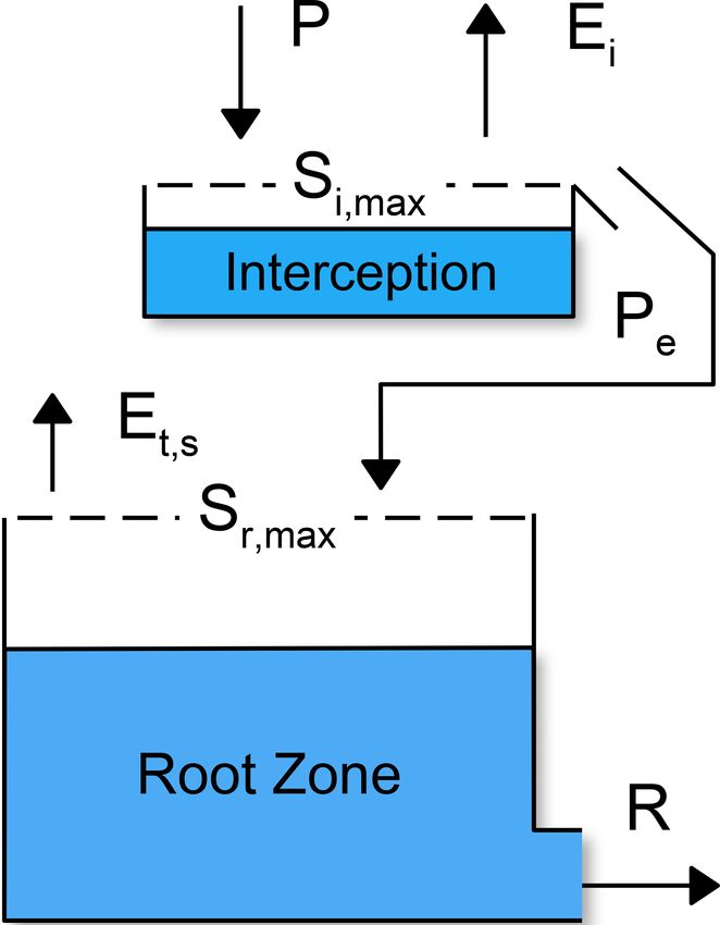
2938                   R. A. Collenteur et al.: Estimating groundwater recharge from groundwater levels using TFN models

Figure 6. Modeling strategy as applied in this study.

objective function is used, minimizing the sum of the squared     3.7   Numerical and software implementation
noise:
                                                                  All models were implemented in Python code and are freely
                                                                  available through the open-source package Pastas (Collen-
         n
         X                                                        teur et al., 2019, version 0.17). The nonlinear model is avail-
Fobj =         υi2 .                                      (14)
         i=1
                                                                  able under the name “FlexModel” in the Pastas library. The
                                                                  nonlinear recharge model is numerically solved using an ex-
   Minimization of the objective function is done using the       plicit Euler scheme with a time step of 1 d. As TFN models
trust-region-reflective algorithm, as implemented in SciPy’s      are traditionally computationally inexpensive and have short
least-squares method (Virtanen et al., 2020, version 1.4.0)       computation times (in the order of seconds), special attention
and Lmfit (Newville et al., 2019, version 1.0). Note that this    was paid to increase the computation speed of the recharge
is not the default option in Lmfit. The standard errors of the    model. This was achieved by using Numba, a just-in-time
parameters are computed from the covariance matrix that is        compiler for Python code (Lam et al., 2015, version 0.49). As
estimated during optimization. An important assumption un-        a result, the nonlinear model has similar computation times
derlying this approach is that the minimized noise series (υ in   to the linear model.
Eq. 13) behaves as normally distributed white noise with no
significant autocorrelation, a constant variance (homoscedas-     3.8   Goodness-of-fit metrics
tic), and a mean of zero. These assumptions were checked
through visual inspection of the results and the use of var-      Four metrics are used to evaluate the goodness-of-fit of the
ious statistical tests for autocorrelation as already shown in    simulated groundwater levels and the groundwater recharge:
the previous section.                                             the mean absolute error (MAE), the root mean squared er-
   The 95% confidence intervals of the simulated recharge         ror (RMSE), the Nash–Sutcliffe efficiency (NSE), and the
are computed through a Monte Carlo simulation (N =                Kling–Gupta efficiency (KGE). The MAE and the RMSE
100 000). Parameter sets are drawn from a multivariate nor-       provide a metric for the overall model fit and error, while the
mal distribution computed using the estimated covariance          NSE is a goodness-of-fit metric commonly used in hydrolog-
matrix. If one of the parameters in a parameter set is out-       ical modeling. The KGE is an aggregate metric and contains
side the parameter boundaries, the set is discarded from the      a correlation term, a bias term, and a variability term (see
sample, and a new parameter set is drawn. This procedure is       Kling et al., 2012, for a more detailed discussion). The NSE
repeated until N parameter sets are available for the Monte       and KGE all have a maximum of 1, denoting a perfect fit of
Carlo simulation. The model is run with the N different pa-       the model with the data. The MAE and RMSE improve when
rameters sets, and the 95 % confidence intervals are com-         moving towards zero.
puted from the ensemble of simulated recharge fluxes.

Hydrol. Earth Syst. Sci., 25, 2931–2949, 2021                                      https://doi.org/10.5194/hess-25-2931-2021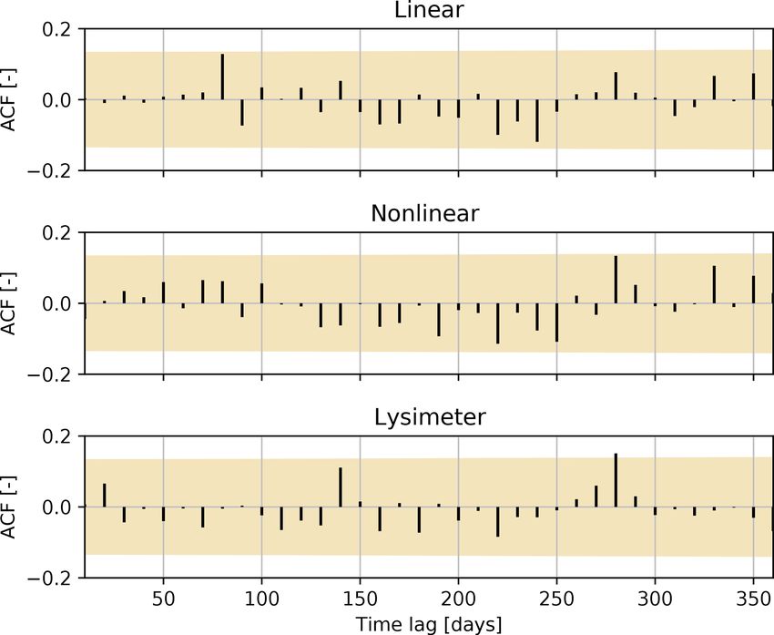
R. A. Collenteur et al.: Estimating groundwater recharge from groundwater levels using TFN models 2939
Table 1. Goodness-of-fit metrics for the groundwater-level simu- Table 2. Performance metrics for the similarity between the esti-
lation for each model. The metrics are computed for the calibra- mated recharge and the measured recharge, in millimeters per 10 d.
tion period (2007–2016) and the validation period (2017–2019). The metrics are shown for the calibration period (2007–2016) and
Groundwater-level measurements with a 10 d time interval were the validation period (2017–2019).
used to calculate these metrics, similar to the measurements used
for calibration. Linear Nonlinear
Linear Nonlinear Lysimeter Cal. Val. Cal. Val.
Cal. Val. Cal. Val. Cal. Val. MAE [mm] 18.76 14.83 5.81 4.92
RMSE [mm] 25.34 20.46 9.38 8.95
MAE [m] 0.17 0.14 0.13 0.13 0.18 0.18 NSE [–] −1.64 −1.96 0.64 0.43
RMSE [m] 0.20 0.19 0.15 0.18 0.23 0.24 KGE [–] 0.27 0.22 0.67 0.60
NSE [–] 0.74 0.73 0.85 0.75 0.64 0.57
KGE [–] 0.86 0.76 0.93 0.77 0.74 0.81
computing the same goodness-of-fit metrics (Table 2). The
4 Results recharge flux computed by the nonlinear model shows a rea-
sonably good fit resulting in, for example, a Kling–Gupta
4.1 Groundwater-level simulations efficiency of KGE = 0.67 for the calibration period. The
recharge computed by the linear model, however, deviates
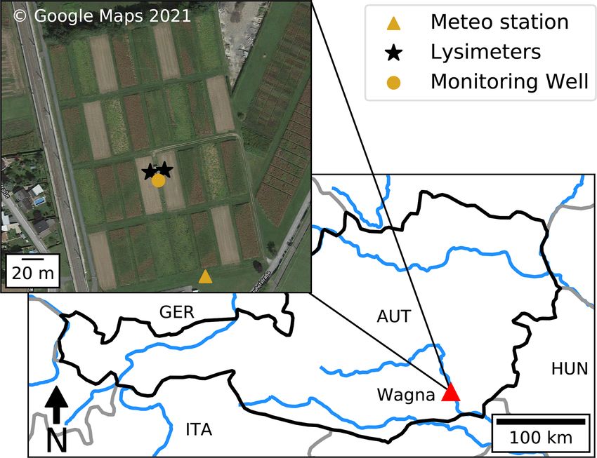
The 10-year period 2007–2016 was used for calibration, and strongly from the lysimeter recharge and often simulates neg-
the 3-year period 2017–2019 was used for model valida- ative recharge that was not measured with the lysimeters. It
tion. The year 2006 was used for model warm-up. The use is concluded that the linear model should not be used to es-
of a warm-up period is especially important for the nonlin- timate groundwater recharge at this small timescale (10 d in-
ear model because the recharge flux strongly depends on the tervals), as expected. For the simulation of groundwater lev-
initial saturation level of the root zone. The simulated and els, the linear model may still be appropriate, as the differ-
the observed groundwater levels are shown in Fig. 7a, along ence in the recharge flux can be compensated for by the shape
with the estimated recharge fluxes (Fig. 7b and c) and the of the response function. This is clearly the case here, as is
measured recharge (Fig. 7d). As the models are calibrated on visible by the differences in the block and step response func-
groundwater-level observations with a 10 d time step, only tions calibrated for each model (shown in Fig. 8). The linear
recharge rates summed over 10 d intervals are presented here. model shows a delayed response to a groundwater recharge
The values of the calibrated parameters can be found in Ta- impulse, whereas the nonlinear and lysimeter models simu-
ble A1 in the Appendix. late an instantaneous response of the groundwater levels.
All three TFN models are able to capture the major Although the linear recharge model in combination with
groundwater dynamics and simulate the observed ground- the four-parameter response function works well to simu-
water levels reasonably well. For the calibration period, the late most of the groundwater levels time series, the model
nonlinear model shows the best simulation of the groundwa- fails under conditions where evaporation is limited by the
ter levels as quantified by the four goodness-of-fit metrics availability of soil moisture. This occurs for example in the
used in this study (see Table 1). The linear model performs years 2010, 2013, and 2017, when the linear model simu-
better than the lysimeter model according to all four metrics. lates a stronger decline in groundwater levels than was ob-
For the validation period, the differences in the metrics are served. These strong declines in simulated groundwater lev-
not as clear, but the nonlinear model still outperforms the els are caused by continued (modeled) evaporation over the
other models. The lysimeter model captures the single peak summer months, resulting in negative recharge rates (as vis-
in groundwater levels during the validation period better than ible in Fig. 7b) and ultimately lower groundwater levels.
the other models but shows the worst simulation of the low Measurements from the lysimeters (data not shown) show
groundwater levels that follow this peak. The linear model that actual evaporation is only a fraction of the potential
performs better during the period with low groundwater lev- evaporation during those periods. Similar behavior for the
els but overestimates the low groundwater levels observed at simulation of low groundwater levels was found by Beren-
the beginning of the validation period. The nonlinear model drecht et al. (2006), using the same linear recharge model.
generally shows good performance but underestimates the These results confirm that the linear recharge model should
low groundwater levels at the end of the validation period. not be used to simulate groundwater levels under such soil-
While the groundwater levels simulated by the linear moisture-limited conditions.
and nonlinear models are rather similar, the groundwater The nonlinear model performs much better under such
recharge fluxes (R) computed by these two models are soil-moisture-limited conditions and simulates almost no
very different (see Fig. 7b and c). The recharge fluxes are recharge during these periods. The nonlinear model resem-
compared to the recharge measured with the lysimeters by bles the recharge behavior as measured with the lysime-
https://doi.org/10.5194/hess-25-2931-2021 Hydrol. Earth Syst. Sci., 25, 2931–2949, 2021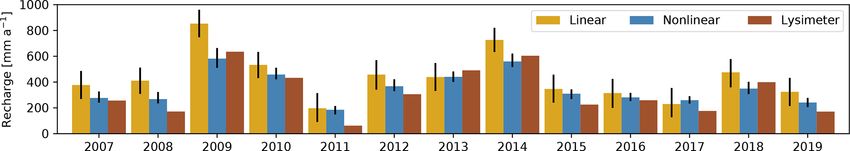
2940                R. A. Collenteur et al.: Estimating groundwater recharge from groundwater levels using TFN models

Figure 7. Observed and simulated groundwater levels (a) and the estimated (b, c) and measured (d) recharge rates (R). The groundwater-
level measurements used for calibration are shown as black dots, and unused measurements are shown as gray dots. The blue shading in plots
(b) and (c) denotes the 95 % confidence intervals of the recharge estimates.

                                                                       ters reasonably well, recharge occurring primarily as indi-
                                                                       vidual events, interspersed with extended periods of reduced
                                                                       recharge. The behavior of event-based recharge was also
                                                                       found in other studies (Groenendijk et al., 2014; Reszler and
                                                                       Fank, 2016) and suggests that recharge paths are activated
                                                                       when a certain threshold in the soil moisture is exceeded.
                                                                       This nonlinear response of recharge to infiltrating precipita-
                                                                       tion also becomes clear when examining the estimated values
                                                                       for the parameter γ , which indicates a nonlinear response
                                                                       with a value of γ = 2.91 [–]. The results show that the use
Figure 8. Calibrated block and step response functions for all three   of a nonlinear recharge model improves the simulation of
models. The block response (a) shows how the groundwater levels        groundwater levels at the study site while also providing a
react to a 1 d recharge event of 1 mm. The step response (b) shows     reasonable estimate of the recharge flux R at this timescale.
the response of the groundwater level to a sudden unit increase in        It is somewhat surprising that the lysimeter model does not
recharge that extends infinitely in time.                              outperform the other two models. Three periods with deviat-
                                                                       ing groundwater levels that stand out in particular are dis-
                                                                       cussed here: the low groundwater levels in 2011, the peak in
                                                                       2013, and a low in 2015. As the groundwater-level fluctua-

Hydrol. Earth Syst. Sci., 25, 2931–2949, 2021                                            https://doi.org/10.5194/hess-25-2931-2021
R. A. Collenteur et al.: Estimating groundwater recharge from groundwater levels using TFN models 2941
Table 3. Descriptive statistics of the deviation (in mm) between The overestimation of recharge by the linear model can be
measured and estimated annual groundwater recharge rates. explained by an underestimation of evaporation that results
from a low value for the evaporation factor f in Eq. (5), f =
Linear Nonlinear −0.69. From the actual evaporation flux computed from the
Mean 114.95 29.99 lysimeter data (Klammler and Fank, 2014), however, it was
Min −51.89 −53.80 calculated that the actual evaporation is approximately 88 %
Max 238.94 123.42 of the potential evaporation (or, f = 0.88) for the period
SD 74.17 62.71 2007–2019. These results confirm findings from Obergfell
et al. (2019) that the factor f is difficult to estimate and
hampers the accurate estimation of recharge using the linear
tions are primarily the result of individual recharge events, model.
and the groundwater system has a long memory, such pe- An accurate estimate of evaporation is also important for
riods with groundwater levels deviating for a longer period recharge estimates made with the nonlinear model. In Fig. 10
of time are likely the result of errors in the quantification the annual cumulative sums of recharge and actual evapo-
of individual recharge events. In 2011, almost no recharge ration are shown as simulated by the nonlinear model and
was recorded in the lysimeters, coinciding with an under- measured with the lysimeters (computed from 1 January
estimation of the simulated groundwater levels. From the to 31 December). The actual evaporation computed by the
groundwater-level measurements, however, it is clear that model is close to that measured with the lysimeters, aver-
some recharge must have taken place, visible by temporarily aging 81 % of the potential evaporation. The vegetation co-
stagnating and even slightly increasing groundwater levels efficient kv in Eq. (6) is calibrated at kv = 1.48 [–], which
during that period. Due to a technical issue with the lysime- seems quite high at first. For most of the simulation period,
ters, no groundwater recharge was recorded by the lysime- however, the saturation of the root zone (Sr /Sr, max ) is well
ters for parts of 2015, explaining the deviation in simulated below the level (lp = 0.25) where evaporation from the root
groundwater levels in that year. No explanation could be zone equals the potential evaporation that is left after inter-
found for the peak in 2013, but this may just as well be an ception evaporation, as visible in Fig. 10c. As a result, the
error in the measurement of a single event, causing a long- actual evaporation simulated by the nonlinear model is still
term deviation in the groundwater-level simulation. below the potential evaporation but matches the actual evap-
oration measured with the lysimeters rather well.
4.2 Annual recharge rates In Fig. 10 it is visible that for years where the actual
evaporation computed by the nonlinear model more or less
Groundwater resource managers are often interested in an- equals the actual evaporation measured with the lysimeter,
nual recharge rates. In this section the ability of the models the recharge fluxes match better as well. When actual evap-
to estimate recharge at this timescale is investigated. The an- oration is underestimated by the model, the recharge is over-
nual recharge rates computed by the TFN models and the estimated (see, e.g., 2008, 2011, and 2015), relative to the
annual recharge measured with the lysimeters are shown in lysimeter recharge. A probable cause for the underestima-
Fig. 9. The nonlinear model performs better than the linear tion of evaporation is the cultivation of different crops in the
model, also shown by the descriptive statistics of the devia- lysimeters during the observation period (shown in the ta-
tion [mm] between measured and estimated annual ground- ble below the plots in Fig. 10). For example, for all years
water recharge rates shown in Table 3. This is particularly when triticale was planted, the actual evaporation was un-
true for wet years, for which the linear model shows large derestimated and the recharge overestimated. As grass ref-
deviations (up to 239 mm yr−1 ) in the annual recharge rates. erence evaporation was used as input data, and the vegeta-
The largest deviation for the nonlinear model occurs during tion coefficient kv is assumed to be constant through time,
the dry year of 2011 (123 mm yr−1 ). The recharge computed the different evaporative capacities of the individual crops
with the linear model has much wider confidence intervals, is not considered in the current model setup. Cultivation of
despite (or maybe because of) having only one calibration pa- different crops does not only influence the total yearly evap-
rameter (f in Eq. 5). This means that the practical use of the oration, but also the pattern in time as a result of different
recharge estimate from the linear model may be limited, as growing seasons and harvest times. Such effects can again
any analysis that uses this estimate as input data would have be observed for triticale, a crop that starts transpiring early in
large uncertainties in its outcomes due to the uncertainty in the year, visible by an earlier rise of the cumulative evapora-
the input data. The nonlinear model performs much better in tion in years when triticale is planted. The use of improved
this respect. input data for evaporation, taking into account the impact of
The long-term average recharge (calculated for the period vegetation on this flux, may further improve recharge estima-
2007–2019) estimated by the nonlinear model (352 mm d−1 ) tions and groundwater-level simulations, particularly in agri-
is much closer to the recharge measured with the lysimeters cultural areas with crop rotation schemes.
(322 mm d−1 ) than to that of the linear model (437 mm d−1 ).
https://doi.org/10.5194/hess-25-2931-2021 Hydrol. Earth Syst. Sci., 25, 2931–2949, 20212942 R. A. Collenteur et al.: Estimating groundwater recharge from groundwater levels using TFN models
Figure 9. Annual recharge rates as computed by each TFN model and as measured with the lysimeters. The error bars denote the 95 %
confidence intervals of the recharge estimate.
Figure 10. Yearly cumulative sums of recharge (a), the actual and potential evaporation (b), and the saturation of the root zone (c). The
dashed line in plot (c) denotes the value of lp , where the evaporation from the root zone will equal the potential evaporation.
4.3 Parameter estimation and consistency of model tions (see Fig. A3 in the Appendix). The parameter values
output for all models are of the same order of magnitude, and model
performance measured as NSE is relatively stable, but the
optimal parameter values can differ significantly from each
The results presented so far are based on the calibration of other between calibrations (e.g., for the nonlinear model ks
the models using only 1 out of every 10 groundwater-level ranges between 100 and 250 mm d−1 ), even though the es-
measurements. The use of only a selection of the available timated confidence intervals overlap for the most part. The
groundwater-level measurements during calibration allowed results of this split-sample test raise the question of param-
for a further investigation into the consistency of the model- eter identifiability. Given the similarity in simulated ground-
ing results, by calibrating the models to 10 different selec- water levels and annual recharge estimates, it is clear that
tions derived of the original time series as a type of split- different combinations of parameters yield similar results. It
sample test. This way, it is possible to assess the consis- is noted here that this analysis does not constitute a formal
tency of the estimated parameters and the impact on the sensitivity analysis of the parameters, for example, by vary-
simulated groundwater levels and the annual recharge esti- ing one parameter and analyzing the changes in the estimated
mates for this particular time series. The resulting ensem- recharge or simulated groundwater levels. The results of this
bles of groundwater-level simulations and annual groundwa- split-sample test rather serve as a motivation for such a study
ter recharge estimates are shown in Fig. A2 in the Appendix. and show that caution is needed when interpreting values of
The results show that both the simulated groundwater levels individual (optimal) parameters. Further research is neces-
and the estimated recharge fluxes are consistent between the sary on the identification of parameters, for example through
different calibrations for all models. This should in fact not testing the models on large samples of groundwater time se-
be that surprising, considering that the time series used for ries (similar to, e.g., Perrin et al., 2001).
calibration originate from the same groundwater-level time
series.
What may be more surprising, however, are the differences
in the estimated parameters between the 10 different calibra-
Hydrol. Earth Syst. Sci., 25, 2931–2949, 2021 https://doi.org/10.5194/hess-25-2931-2021R. A. Collenteur et al.: Estimating groundwater recharge from groundwater levels using TFN models 2943
5 Discussion rors of the estimated parameters. Reliable estimates of the
standard errors of the parameters may be obtained in the cur-
5.1 Choice and performance of nonlinear recharge rent framework when the autocorrelation of the minimized
models noise series is removed by using an appropriate noise model.
Here, an AR(1) model did not suffice for this purpose, and an
The results from this study showed that, compared to the lin- ARMA(1,1) noise model was used instead. The current im-
ear model, the nonlinear recharge model is more capable of plementation of the ARMA(1,1) model is for groundwater-
simulating true system dynamics that are commonly not mea- level time series with regular time steps between observa-
sured, such as groundwater recharge and actual evaporation. tions, unlike the AR(1) model that is often used (von Asmuth
This suggests that the improvements in the simulation of the and Bierkens, 2005). Additional work is needed to make
groundwater levels and the estimation of recharge are the re- the ARMA(1,1) model suitable for time series with irregu-
sult of a better representation of the hydrological processes, lar time steps.
rather than the result of added mathematical complexity. As The ARMA(1,1) noise model performed reasonably well
such, the use of nonlinear recharge models in TFN models is in transforming the residual series into a noise time series
a promising step in the effort “to get the right answers for the that is approximately white noise, but some autocorrelation
right reasons”, as advocated by, e.g., Kirchner (2006). This remained in the noise series. As a practical solution, the time
may be particularly important when using this type of mod- interval between groundwater-level measurements was in-
els to forecast groundwater recharge and levels under drought creased to 10 d by removing measurements from the time se-
conditions. ries. It is noted here that the optimal time interval is likely to
It is noted that the nonlinear recharge model developed for be site-specific and should be investigated for each individual
this study is only one of a set of similar soil-water storage time series. The approach shown in Sect. 3.5 can be helpful
models that may be applied. Comparable results (not shown in determining the optimal time step size used for model cali-
here) were obtained using the nonlinear recharge model de- bration. Alternatively, it may be appropriate to use an ARMA
veloped by Berendrecht et al. (2006), which is also available model of higher order (see, e.g., Box and Jenkins, 1970). The
in the Pastas software (Collenteur et al., 2019). It is expected modeling of the residuals and the choice of an appropriate
that other nonlinear models (e.g., the models of Peterson and noise model and time interval are an iterative process, as also
Western, 2014) perform similarly. The identification of the suggested by Smith et al. (2015). Additionally, it is impor-
most appropriate nonlinear recharge model under different tant to use an appropriate length for the calibration period.
conditions is a topic for future investigation. Van der Spek and Bakker (2017) recommended a 10- to 20-
The application of a nonlinear recharge model does come year period for simulating groundwater levels with reliable
with additional challenges in the estimation of the model pa- credible intervals.
rameters. Nonlinear models have a larger number of parame-
ters that need to be estimated and a higher potential for prob- 5.3 Application to other hydrogeological settings
lems related to equifinality (Beven, 2006). As was shown in
this study, however, not all model parameters have to be cal- The presented approach was tested on relatively shallow
ibrated, and some may be fixed to sensible values (following groundwater levels (±4 m depth to the water table), for which
e.g., Savenije, 2010). The use of nonlinear models therefore no feedback between the groundwater and root zone was ex-
does not necessarily imply a higher number of parameters pected. In this setting, an exponential response function was
that need to be calibrated; i.e., the same number of parame- used in the nonlinear model, and the computed flux R could
ters were calibrated for the linear and nonlinear models used be directly interpreted as groundwater recharge. The use of
in this study. Nonetheless, finding the optimal parameter val- an exponential function may not be appropriate for deeper
ues may be challenging and dependent on the initial parame- groundwater bodies with thicker unsaturated zones, which
ter values. Global optimization methods may help overcome require a more complicated response function that accounts
these problems, as for example shown by Peterson and West- for a significant travel time through the unsaturated zone.
ern (2014). In that case, the estimated flux R should be interpreted as
drainage from the root zone to the groundwater and not as
5.2 Transformation of the residuals to uncorrelated recharge occurring at the water table. Alternatively, as sug-
noise gested by Peterson and Fulton (2019), the flux could be “av-
eraged over a period greater than the time lag” between the
In this study, model parameters were estimated by fitting drainage from the root zone and the arrival at the water table,
simulated groundwater levels to observed groundwater lev- to provide an estimate of gross recharge at larger timescales.
els. The recharge is an intermediate model result that is not It is not always possible to assume that there is no feed-
calibrated for. It is recommended here to quantify the im- back between the root zone and the groundwater. If the roots
pact of parameter uncertainties on the recharge estimates by of the vegetation reach the groundwater, for example in shal-
computing their confidence intervals using the standard er- low groundwater systems or deep rooting systems, evapora-
https://doi.org/10.5194/hess-25-2931-2021 Hydrol. Earth Syst. Sci., 25, 2931–2949, 2021You can also read