Groundwater level forecasting with artificial neural networks: a comparison of long short-term memory (LSTM), convolutional neural networks (CNNs) ...
←
→
Page content transcription
If your browser does not render page correctly, please read the page content below
Hydrol. Earth Syst. Sci., 25, 1671–1687, 2021
https://doi.org/10.5194/hess-25-1671-2021
© Author(s) 2021. This work is distributed under
the Creative Commons Attribution 4.0 License.

Groundwater level forecasting with artificial neural networks:
a comparison of long short-term memory (LSTM),
convolutional neural networks (CNNs), and non-linear
autoregressive networks with exogenous input (NARX)
Andreas Wunsch1 , Tanja Liesch1 , and Stefan Broda2
1 Hydrogeology,   Karlsruhe Institute of Technology (KIT), Institute of Applied Geosciences,
Kaiserstr. 12, 76131 Karlsruhe, Germany
2 Federal Institute for Geosciences and Natural Resources (BGR), Wilhelmstr. 25–30, 13593 Berlin, Germany

Correspondence: Andreas Wunsch (andreas.wunsch@kit.edu)

Received: 23 October 2020 – Discussion started: 23 November 2020
Revised: 1 February 2021 – Accepted: 2 March 2021 – Published: 1 April 2021

Abstract. It is now well established to use shallow artifi-       tialization effects, which nevertheless can be handled easily
cial neural networks (ANNs) to obtain accurate and reli-          using ensemble forecasting. We showed that shallow neural
able groundwater level forecasts, which are an important tool     networks, such as NARX, should not be neglected in compar-
for sustainable groundwater management. However, we ob-           ison to DL techniques especially when only small amounts
serve an increasing shift from conventional shallow ANNs to       of training data are available, where they can clearly outper-
state-of-the-art deep-learning (DL) techniques, but a direct      form LSTMs and CNNs; however, LSTMs and CNNs might
comparison of the performance is often lacking. Although          perform substantially better with a larger dataset, where DL
they have already clearly proven their suitability, shallow re-   really can demonstrate its strengths, which is rarely available
current networks frequently seem to be excluded from the          in the groundwater domain though.
study design due to the euphoria about new DL techniques
and its successes in various disciplines. Therefore, we aim
to provide an overview on the predictive ability in terms of
                                                                  1   Introduction
groundwater levels of shallow conventional recurrent ANNs,
namely non-linear autoregressive networks with exogenous          Groundwater is the only possibility for 2.5 billion peo-
input (NARX) and popular state-of-the-art DL techniques           ple worldwide to cover their daily water needs (UNESCO,
such as long short-term memory (LSTM) and convolutional           2012). and at least half of the global population uses ground-
neural networks (CNNs). We compare the performance on             water for drinking-water supplies (WWAP, 2015). More-
both sequence-to-value (seq2val) and sequence-to-sequence         over, groundwater also constitutes for a substantial amount
(seq2seq) forecasting on a 4-year period while using only         of global irrigation water (FAO, 2010), which altogether
few, widely available and easy to measure meteorological in-      and among other factors such as population growth and cli-
put parameters, which makes our approach widely applica-          mate change make it a vital future challenge to dramati-
ble. Further, we also investigate the data dependency in terms    cally improve the way of using, managing, and sharing wa-
of time series length of the different ANN architectures. For     ter (WWAP, 2015). Accurate and reliable groundwater level
seq2val forecasts, NARX models on average perform best;           (GWL) forecasts are a key tool in this context, as they pro-
however, CNNs are much faster and only slightly worse in          vide important information on the quantitative availability of
terms of accuracy. For seq2seq forecasts, mostly NARX out-        groundwater and can thus form the basis for management de-
perform both DL models and even almost reach the speed            cisions and strategies.
of CNNs. However, NARX are the least robust against ini-

Published by Copernicus Publications on behalf of the European Geosciences Union.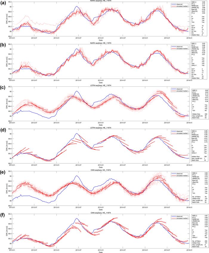
1672                                       A. Wunsch et al.: Groundwater level forecasting with LSTM, CNNs, and NARX

   Especially due to the success of deep-learning (DL) ap-         Müller et al. (2020), who focus on hyperparameter optimiza-
proaches in recent years and their more and more widespread        tion, draw the conclusion that CNN results are less robust
application in our daily life, DL is starting to transform tra-    compared to LSTM predictions; however, other analyses in
ditional industries and is also increasingly used across mul-      their study also show better results of CNNs compared to
tiple scientific disciplines (Shen, 2018). This applies as well    LSTMs. Jeong and Park (2019) conducted a comparison of
to water sciences, where machine learning methods in gen-          NARX and LSTM (and others) performance on groundwa-
eral are used in a variety of ways, as data-driven approaches      ter level forecasting. They found both NARX and LSTM to
offer the possibility to directly address questions on relation-   be the best models in their overall comparison concerning
ships between relevant input forcings and important system         the prediction accuracy; however, they used a deep NARX
variables, such as run-off or groundwater level, without the       model with more than one hidden layer. To the best of the au-
need to build classical models and explicitly define physical      thors’ knowledge, no direct comparison has yet been made of
relationships. This is especially handy because these classi-      (shallow) NARX, LSTMs, and CNNs to predict groundwater
cal models might sometimes be oversimplified or (in the case       levels.
of numerical models) data hungry, difficult, time-consuming           In this study we aim to provide an overview on the predic-
to set up and maintain, and therefore expensive. In partic-        tive ability in terms of groundwater levels of shallow conven-
ular artificial neural networks (ANNs) have been success-          tional recurrent ANNs, namely NARX and popular state-of-
fully applied to research related to a variety of surface-water    the-art DL techniques LSTM and (1D) CNNs. We compare
(Maier et al., 2010) and groundwater-level (Rajaee et al.,         the performance of both on single-value (sequence-to-value;
2019) questions already; however, especially DL was used           also known as one-step-ahead, sequence-to-one, or many-to-
only gradually at first (Shen, 2018) but is just about to take     one forecasting) and sequence (sequence-to-sequence) fore-
off, which is reflected in the constantly increasing number of     casting. We use data from 17 groundwater wells within the
DL and water-resource-related publications (see e.g. Chen          Upper Rhine Graben region in Germany and France, which
et al., 2020; Duan et al., 2020; Fang et al., 2019, 2020;          was selected based on prior knowledge and representing the
Gauch et al., 2020, 2021; Klotz et al., 2020; Kraft et al.,        full bandwidth of groundwater dynamic types in the region.
2020; Kratzert et al., 2018, 2019a, b; Pan et al., 2020; Rah-      Further, we use only widely available and easy-to-measure
mani et al., 2021). In this work we explore and compare            meteorological input parameters (precipitation, temperature,
the abilities of non-linear autoregressive networks with ex-       and relative humidity), which makes our approach widely
ogenous input (NARX), which have been successfully ap-             applicable. All models are optimized using Bayesian opti-
plied multiple times to groundwater level forecasting in the       mization models, which we extend to also solve the common
past and to the currently popular DL approaches of long            input parameter selection problem by considering the inputs
short-term memory (LSTM) and convolutional neural net-             as optimizable parameters. Further, the data dependency of
works (CNNs).                                                      all models is explored in a simple experimental setup for
   During the last years several authors have shown the abil-      which there are substantial differences in shallow- and deep-
ity of NARX to successfully model and forecast groundwa-           learning models in the need for training data, as one might
ter levels (Alsumaiei, 2020; Chang et al., 2016; Di Nunno          suspect.
and Granata, 2020; Guzman et al., 2017, 2019; Hasda et al.,
2020; Izady et al., 2013; Jeihouni et al., 2019; Jeong and
Park, 2019; Wunsch et al., 2018; Zhang et al., 2019). Al-          2     Methodology
though LSTMs and CNNs are state-of-the-art DL techniques
and commonly applied in many disciplines, they are not yet         2.1    Input parameters
widely adopted in groundwater level prediction applications,
except within the last 2 years. Thereby, LSTMs were used           In this study we only use the meteorological input vari-
twice as often to predict groundwater levels (Afzaal et al.,       ables precipitation (P ), temperature (T ), and relative humid-
2020; Bowes et al., 2019; Jeong et al., 2020; Jeong and Park,      ity (rH), which in general are widely available and easy to
2019; Müller et al., 2020; Supreetha et al., 2020; Zhang et al.,   measure. In principle, this makes this approach easily trans-
2018) compared to CNNs (Afzaal et al., 2020; Lähivaara             ferable and thus applicable almost everywhere. Precipitation
et al., 2019; Müller et al., 2020). The main reason might be       may serve as a surrogate for groundwater recharge; tempera-
that the strength of CNNs is mainly the extraction of spatial      ture and relative humidity include the relationship with evap-
information from image-like data, whereas LSTMs are es-            otranspiration and at the same time provide the network with
pecially suited to process sequential data, such as from time      information on seasonality due to the usually distinct annual
series. Overall, these studies show that LSTMs and CNNs are        cycle. As an additional synthetic input parameter, a sinu-
very well suited to forecast groundwater levels. Both Afzaal       soidal signal fitted to the temperature curve (Tsin ) can pro-
et al. (2020) and Müller et al. (2020) also directly compared      vide the model with noise-free information on seasonality,
the performance of LSTMs and CNNs, but no clear superi-            which often allows for significantly improved predictions to
ority of one over the other can be drawn from their results.       be made (Kong-A-Siou et al., 2014). Without doubt, the most

Hydrol. Earth Syst. Sci., 25, 1671–1687, 2021                                       https://doi.org/10.5194/hess-25-1671-2021
A. Wunsch et al.: Groundwater level forecasting with LSTM, CNNs, and NARX                                                    1673

important input parameter out of these is P , since groundwa-     also contain a short-term memory, i.e. delay vectors for each
ter recharge usually has the greatest influence on groundwa-      input (and feedback), which allow for the availability of sev-
ter dynamics. Therefore, P is used always as input param-         eral input time steps simultaneously, depending on the length
eter; the suitability of the remaining parameters is checked      of the vector. Usually, delays are crucial for the performance
and optimized for each time series and each model individ-        of NARX models. Please note that some of our experiments
ually. The fundamental idea is that for wells with primar-        include past GWLs for training (compare Sect. 2.1), which is
ily natural groundwater dynamics, the relationship between        also performed in closed-loop setup and thus uses both mul-
groundwater levels and the important processes of ground-         tiple observed past GWLs (according to the size of the input
water recharge and evapotranspiration should be mapped via        delay) as an input, as well as multiple simulated GWLs (ac-
the meteorological parameters P , T , and rH. However, espe-      cording to the size of the feedback delay) via the feedback
cially for wells with a dynamic influenced by other factors,      connection. In a way this mimics the open-loop setup; how-
this is usually only valid to a limited extent, since groundwa-   ever, we still use the feedback connection and simply treat
ter dynamics can depend on various additional factors such        the past observed GWL as an additional input.
as groundwater extractions or surface water interactions. Due        The given configuration describes sequence-to-value fore-
to a typically strong autocorrelation of groundwater level        casting. To perform sequence-to-sequence forecasts, some
time series, a powerful predictor for the future groundwater      modifications are necessary. As other ANNs, NARX are ca-
level is the groundwater level in the past. Depending on the      pable of performing forecasts of a complete sequence at
purpose and methodological setup, it does not always make         once; i.e. one output neuron predicts a vector with multiple
sense to include this parameter; however, where meaningful        values. Technically it is necessary to use the same length for
we explored also past GWL as inputs.                              input and output sequences. To build and apply NARX mod-
                                                                  els, we use MATLAB 2020a (Mathworks Inc., 2020) and its
2.2   Nonlinear autoregressive exogenous model (NARX)             Deep Learning Toolbox.

Non-linear autoregressive models with exogenous input re-         2.3   Long short-term memory (LSTM)
late the current value of a time series to past values of the
same time series, as well as to current and past values of ad-    Long short-term memory networks are recurrent neural net-
ditional exogenous time series. We implement this type of         works which are widely applied to model sequential data
model as a recurrent neural network (RNN), which extends          like time series or natural language. As stated, RNNs suf-
the well-known feed-forward multilayer perceptron struc-          fer from the vanishing gradient problem during backpropa-
ture (MLP) by a global feedback connection between output         gation, and in the case of simple RNNs, their memory barely
and input layers. One can therefore also refer to it as recur-    includes the previous 10 time steps (Bengio et al., 1994).
rent MLP. NARX are frequently applied for non-linear time         LSTMs, however, can remember long-term dependencies be-
series prediction and non-linear filtering tasks (Beale et al.,   cause they have been explicitly designed to overcome this
2016). Similar to other types of RNNs, NARX have also             problem (Hochreiter and Schmidhuber, 1997). Besides the
difficulties in capturing long-term dependencies due to the       hidden state of RNNs, LSTMs have a cell memory (or cell
problem of vanishing and exploding gradients (Bengio et al.,      state) to store information and three gates to control the infor-
1994), yet they can keep information up to 3 times longer         mation flow (Hochreiter and Schmidhuber, 1997). The forget
than simple RNNs (Lin et al., 1996a, b), so they can con-         gate (Gers et al., 2000) controls which and how much infor-
verge more quickly and generalize better in comparison (Lin       mation of the cell memory is forgotten, the input gate con-
et al., 1998). Using the recurrent connection, future outputs     trols which inputs are used to update the cell memory, and
are both regressed on independent inputs and on previous          the output gate controls which elements of the cell mem-
outputs (groundwater levels in our case), which is the stan-      ory are used to update the hidden state of the LSTM cell.
dard configuration for multi-step prediction and also known       The cell memory enables the LSTM to handle long-term de-
as closed-loop configuration. However, NARX can also be           pendencies, because information can remain in the memory
trained by using the open-loop configuration, where the ob-       for many steps (Hochreiter and Schmidhuber, 1997). Several
served target is presented as an input instead of feeding back    LSTM layers can be stacked on top of each other in a model;
the estimated output. This configuration can make training        however, the last LSTM layer is followed by a traditional
more accurate and efficient, as well as computationally less      fully connected dense layer, which in our case is a single
expensive, because learning algorithms do not have to handle      output neuron that outputs the groundwater level. To real-
recurrent connections (Moghaddamnia et al., 2009). How-           ize sequence forecasting, as many output neurons in the last
ever, experience shows that both configurations can be ad-        dense layer as steps in the sequence are needed. For LSTMs,
equate for training a NARX model, since open-loop training        we rely on Python 3.8 (van Rossum, 1995) in combination
often results in more accurate performance in terms of mean       with the libraries Numpy (van der Walt et al., 2011), Pan-
errors, whereas closed-loop trained models often are better       das (McKinney, 2010; Reback et al., 2020), scikit-learn (Pe-
in capturing the general dynamics of a time series. NARX          dregosa et al., 2011), and Matplotlib (Hunter, 2007). Further,

https://doi.org/10.5194/hess-25-1671-2021                                      Hydrol. Earth Syst. Sci., 25, 1671–1687, 2021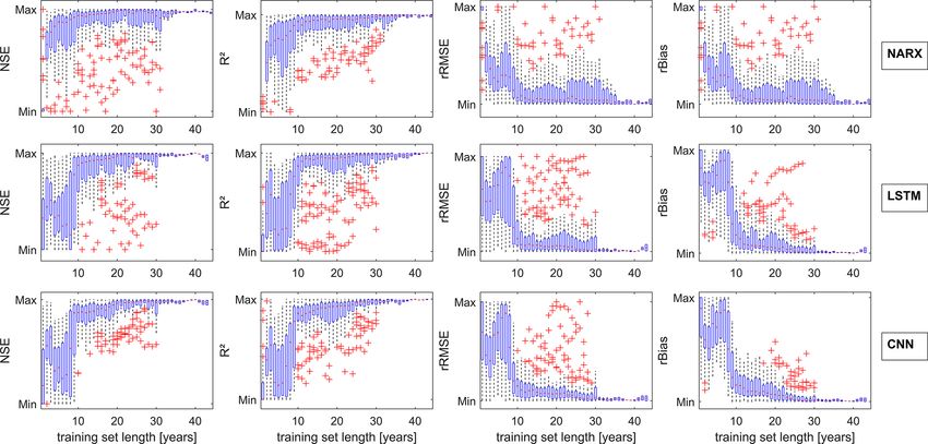
1674                                        A. Wunsch et al.: Groundwater level forecasting with LSTM, CNNs, and NARX

we use the deep-learning frameworks TensorFlow (Abadi               a Bayesian model are the number of units within the LSTM
et al., 2015) and Keras (Chollet, 2015).                            layer (hidden size, 1 to 256), the batch size (1 to 256), and the
                                                                    sequence length (1 to 52). The latter can be interpreted more
2.4    Convolutional neural networks (CNNs)                         or less as equivalent to the delay size of the NARX models
                                                                    and is often referred to as the number of inputs (Fig. 1).
CNNs are neural networks established by LeCun et al. (2015)            The CNN models we apply consist of one convolutional
and are predominantly used for image recognition and classi-        layer, a max-pooling layer, and two dense layers, where
fication. However, they also work well on signal processing         the second one consists only of one neuron in the case of
tasks and are used for natural language processing for ex-          sequence-to-value forecasting. The Adam optimizer is used
ample. CNNs usually comprise three different layers. Con-           with the same configuration as for the LSTM models. For
volutional layers, the first type, consist of filters and feature   all CNN models, we use a kernel size of 3 and optimize the
maps. The input to a filter is called receptive field and has       batch size (1 to 256), sequence length (1 to 52), the number
a fixed size. Each filter is dragged over the entire previous       of filters (1 to 256) within the convolutional layer, and the
layer resulting in an output, which is collected in the fea-        number of neurons within the first dense layer (dense size, 1
ture map. Convolutional layers are often followed by pool-          to 256) according to a Bayesian optimization model (Fig. 1).
ing layers that perform downsampling of the previous layers            Hyperparameter optimization is conducted by applying
feature map; thus, information is consolidated by moving a          Bayesian optimization using the Python implementation by
receptive field over the feature map. Such fields apply simple      Nogueira (2014). We apply 50 optimization steps as a mini-
operations like averaging or maximum selection. Similar to          mum (25 random exploration steps followed by 25 Bayesian
LSTM models, multiple convolutional and pooling layers in           optimization steps). After that, the optimization stops as soon
varying order can be stacked on top of each other in deeper         as no improvement has been recorded during 20 steps or
models. The last layer is followed by a fully connected dense       after a maximum of 150 steps. For the NARX models, we
layer with one or several output neurons. To realize sequence       use the MATLAB built-in Bayesian optimization, where the
forecasting, as many output neurons in the last dense layer         first 50 steps cannot be distinguished as explained; how-
as steps in the sequence are needed. For CNNs, we equally           ever, the rest applies accordingly. The acquisition function
use Python 3.8 (van Rossum, 1995) in combination with the           in all three cases is expected improvement, and the optimiza-
above-mentioned libraries and frameworks.                           tion target function we chose is the sum of Nash–Sutcliffe
                                                                    efficiency (NSE) and squared Pearson’s correlation coeffi-
2.5    Model calibration and evaluation                             cient (R 2 ) (compare Eqs. 1 and 2), because these two criteria
                                                                    are very important and well-established criteria for assessing
In this study we use NARX models with one hidden layer,             the forecast accuracy in water-related contexts.
and we train them in a closed loop using the Levenberg–                All three model types use 30 as the maximum number of
Marquardt algorithm, which is a fast and reliable second-           training epochs. To prevent overfitting, we apply early stop-
order local method (Adamowski and Chan, 2011). We                   ping with a patience of 5 steps. The testing or evaluation pe-
choose closed-loop configuration for training, because other        riod in this study for all models are the years 2012 to 2015 in-
hyperparameters (HPs) are optimized using a Bayesian                clusively. This period is exclusively used for testing the mod-
model (see below), which seems to work properly only in             els. The data before 2012 are of varying length (hydrographs
closed-loop configuration, probably due to the artificially         start between 1967 and 1994; see also Fig. 3), depending on
pushed training performance in open-loop configuration. Op-         the available data, and are split into three parts, namely 80 %
timized HPs are the inputs T , Tsin , and rH (1/0, i.e. yes/no);    for training, 10 % for early stopping, and 10 % for testing
size of the input delays (ID P , ID T , ID Tsin , ID rH); size      during HP optimization (denoted the opt-set) (Fig. 2). Thus,
of the feedback delay vector (F D); and number of hidden            the target function of the HP-optimization procedure is only
neurons (hidden size). Delays (ID and F D) can take values          calculated on the opt-set.
between 1 and 52 (which is 1 year of weekly data); the num-            All data are scaled between −1 and 1 and all models
ber of hidden neurons is optimized between 1 and 20. Strictly       are initialized randomly and show therefore a dependency
speaking, input selection is not a hyperparameter optimiza-         towards the random number generator seed. To minimize
tion problem; however, the algorithm can also be applied to         initialization influence, we repeat every optimization step
select an appropriate set of inputs (Fig. 1). This assumption       five times and take the mean of the target function. For the
applies in our study also to LSTM and CNN models.                   final model evaluation in the test period (2012–2016), we
   We choose our LSTM models to consist of one LSTM                 use 10 pseudo-random initializations and calculate errors of
layer, followed by a fully connected dense layer with a sin-        the median forecast. For seq2seq forecasting, we always take
gle output neuron in the case of sequence-to-value forecast-        the median performance over all forecasted sequences, which
ing. We use the Adam optimizer with an initial learning rate        have a length of 3 months or 12 steps. This is a realistic length
of 1 × 10⁻³ and apply gradient clipping to prevent gradi-           for direct sequence forecasting of groundwater levels, which
ents from exploding. Hyperparameters being optimized by             also has some relevance in practice, because it (i) provides

Hydrol. Earth Syst. Sci., 25, 1671–1687, 2021                                        https://doi.org/10.5194/hess-25-1671-2021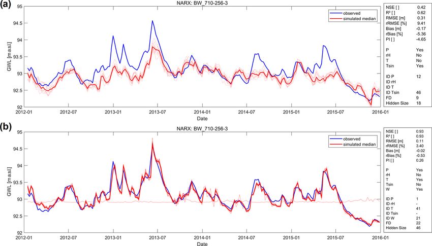
A. Wunsch et al.: Groundwater level forecasting with LSTM, CNNs, and NARX 1675
Figure 1. (a) Simplified schematic summary of the models and their structures used in this work. ID and FD are delays, circles in dense
layers symbolize neurons, and squares within the LSTM cell represent the number of hidden units. (b) Hyperparameters (and inputs) of
each model used to tune the models by using Bayesian optimization algorithm; the last column summarizes the optimization ranges for each
parameter.
n
(oi − pi )2
P
i=1
NSE = 1 − n (1)
(oi − o)2
P
i=1
Please note that in the denominator we use the mean ob-
Figure 2. Data splitting scheme: each time series is split into four served values until the start of the test period (2012 in the
parts for training, early stopping, HP optimization, and testing. The case of our final model evaluation). This best represents the
latter is fixed to the period years 2012 to 2016 for all wells; the meaning of the NSE, which compares the model perfor-
former three parts depend on the available time series length. mance to the mean values of all known values at the time
of the start of the forecast.
2
useful information for many decision-making applications
Pn
(e.g. groundwater management) and (ii) is also an established (oi − o) (pi − p)
time span in meteorological forecasting, known as seasonal 2
i=1
R = s s (2)
forecasts. In principle, this also allows for a performance n n
P 2 P 2
(oi − o) (pi − p)
comparison of 12-step seq2seq forecasts with a potential 12- i=1 i=1
step seq2val forecast, based on operational meteorological
forecasting, where the input uncertainty potentially lowers In our case, we use the squared Pearson correlation co-
the groundwater level forecast performance. However, this efficient R 2 as a general coefficient of determination, since
is beyond the scope of this study, which focuses on neural it compares the linear relation between simulated and ob-
network architecture comparison. served GWLs.
To judge forecast accuracy, we calculate several metrics: v
Nash–Sutcliffe efficiency (NSE), squared Pearson’s correla- u n
u1 X
tion coefficient (R 2 ), absolute and relative root mean squared RMSE = t (oi − pi )2 , (3)
n i=1
errors (RMSE and rRMSE, respectively), absolute and rela-
tive biases (Bias and rBias, respectively), and the persistency
v
u n
u1 X 2
index (PI). For the following equations, it applies that o rep- oi − pi
rRMSE = t , (4)
resents observed values, p represents predicted values, and n i=1 omax − omin
n stands for the number of samples.
https://doi.org/10.5194/hess-25-1671-2021 Hydrol. Earth Syst. Sci., 25, 1671–1687, 2021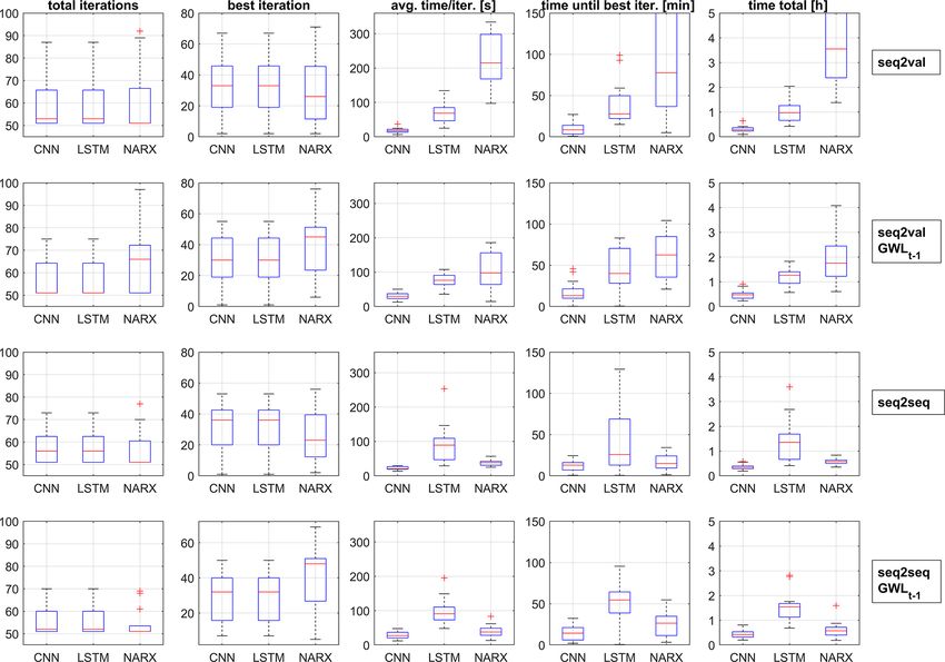
1676                                        A. Wunsch et al.: Groundwater level forecasting with LSTM, CNNs, and NARX

        1X n                                                        LSTMs is the preferred option. For CNNs, we observed a
Bias =        (oi − pi ) ,                                   (5)    substantially faster calculation (factor 2 to 3) on the CPU and
        n i=1
                                                                    therefore favoured this option. Both LSTMs and CNNs were
            n
         1X        oi − pi                                          built and applied using Python 3.8, and the GPU we used for
rBias =                      ,                               (6)
         n i=1 omax − omin                                          LSTMs was a Nvidia GeForce RTX 2070 Super.
            n
                 (oi − pi )2
            P
           i=1                                                      3     Data and study area
PI = 1 −   n                      .                          (7)
                 (oi − olast )2
           P
                                                                    In this study we examine the groundwater level forecasting
           i=1                                                      performance at 17 groundwater wells within the Upper Rhine
   Please note that RMSE and Bias are useful to compare per-        Graben (URG) area (Fig. 3), which is the largest groundwa-
formances for a specific time series among different models;        ter resource in central Europe (LUBW, 2006). The aquifers
however, only rRMSE and rBias are meaningful to compare             of the URG cover 80 % of the drinking water demand of
model performance between different time series. The per-           the region as well as the demand for agricultural irrigation
sistency index (PI) basically compares the performance to a         and industrial purposes (Région Alsace – Strasbourg, 1999).
naïve model that uses the last known observed groundwater           The wells are selected from a larger dataset from the region
level at the time the prediction starts. This is particularly im-   with more than 1800 hydrographs. Based on prior knowl-
portant to judge the performance when past groundwater lev-         edge, the wells of this study represent the full bandwidth of
els (GWL(t−1) ) are used as inputs, because especially in this      groundwater dynamics occurring in the dataset. The whole
case the model should outperform a naïve forecast (PI > 0).         dataset mainly consists of shallow wells from the upper-
                                                                    most aquifer within the Quaternary sand/gravel sediments of
2.6    Data dependency                                              the URG. Mean GWL depths are lower than 5 m b.g.l. for
                                                                    70 % of the data, rising to a maximum of about 20–30 m to-
The data dependency of empirical models is a classical re-          wards the Graben edges. The considered aquifers show gen-
search question (Jakeman and Hornberger, 1993), often fo-           erally high storage coefficients and high hydraulic conduc-
cusing on the number of parameters but also concerning the          tivities of the order of 1 × 10⁻⁴ to 1 × 10⁻³ m s−1 (LUBW,
length of available data records. Data scarcity is also an im-      2006). In some areas, e.g. the northern URG, strong an-
portant topic in machine learning in general, especially in         thropogenic influences exist, due to intensive groundwater
deep learning and the focus of recent research (e.g. Gauch          abstractions and management efforts. A list of all exam-
et al., 2021). One can therefore expect to find performance         ined wells with additional information on identifiers and co-
differences between both shallow and deep models used in            ordinates can be found in the Supplement (Table S1). All
this study. We hence performed experiments to explore the           groundwater data are available for free via the web ser-
need for training data for each of the model types. For this,       vices of the local authorities (HLNUG, 2019; LUBW, 2018;
we started with a reduced training record length of only            MUEEF, 2018). The shortest time series starts in 1994 and
2 years before testing the performance on the fixed test set of     the longest in 1967; however, most hydrographs (12) start
4 years (2012–2016). In the following we gradually length-          between 1980 and 1983 (Fig. 3). Meteorological input data
ened the training record until the maximum available length         were derived from the HYRAS dataset (Frick et al., 2014;
for each well and tracked the error measure changes. This ex-       Rauthe et al., 2013), which can be obtained free of charge
periment aims to give an impression of how much data might          for non-commercial purposes on request from the German
be needed to achieve satisfying forecasting performance and         Meteorological Service (DWD, 2021). In this study we ex-
if there are substantial differences between the models; how-       clusively consider weekly time steps for both groundwater
ever, it lies out of the scope of interest to answer this very      and meteorological data.
complex question in a general way for each of the modelling
approaches.
                                                                    4     Results and discussion
2.7    Computational aspects
                                                                    4.1    Sequence-to-value (seq2val) forecasting
We used different computational setups to build and apply                  performance
the three model types. We built the NARX models in MAT-
LAB and performed the calculations on the CPU (AMD-                 Figure 4 summarizes and compares the overall seq2val fore-
Ryzen 9 3900X). The use of a GPU instead of a CPU is                casting accuracy of the three model types for all 17 wells.
not possible for NARX models in our case because of the             Figure 4a shows the performance when only meteorological
Levenberg–Marquardt training algorithm, which is not suit-          inputs are used; the models in Fig. 4b are additionally pro-
able for GPU computation. Both LSTMs and CNNs, how-                 vided with GWLt−1 as an input. Because the GWL of the
ever, can be calculated on a GPU, which in the case of              last step has to be known, the latter configuration has only

Hydrol. Earth Syst. Sci., 25, 1671–1687, 2021                                        https://doi.org/10.5194/hess-25-1671-2021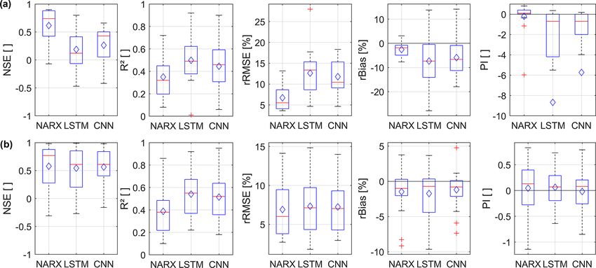
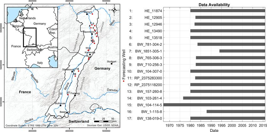
A. Wunsch et al.: Groundwater level forecasting with LSTM, CNNs, and NARX                                                              1677

Figure 3. Study area and positions of examined wells (left), as well as respective time series length for each of the wells (right).

Figure 4. Boxplots showing the seq2val forecast accuracy of NARX, LSTM, and CNN models within the test period (2012–2016) for all
considered 17 hydrographs. The diamond symbols indicate the arithmetic mean; (a) only meteorological inputs; (b) GWLt−1 as additional
input.

limited value for most applications since only one-step-ahead              formance of all three models significantly (Fig. 4b). Addi-
forecasts are possible in a real-world scenario. However, the              tionally, performance differences between the models vanish
inputs of the former configuration are usually available as                and remain only visible as slight tendencies. This is not sur-
forecasts themselves for different time horizons. Figure 4a                prising, as the past groundwater level is usually a good or
shows that on average NARX models perform best, followed                   even the best predictor of the future GWL, at least for one-
by CNN models; LSTMs achieve the least accurate results.                   step-ahead forecasting, and all models are able to use this
This is consistent for all error measures except rBias, where              information. The general superiority of NARX in the case
CNN models show slightly less bias than NARX. However,                     of Fig. 4a is therefore also expected, as a feedback connec-
all models suffer from significant negative bias values of the             tion within the model already provides information on past
same order of magnitude, meaning that GWLs are system-                     groundwater levels, even though it includes also a certain
atically underestimated. Providing information about past                  forecasting error. However, providing GWLt−1 as input to a
groundwater levels up to t − 1 (GWLt−1 ) improves the per-                 seq2val model (Fig. 4b) basically means providing the naïve

https://doi.org/10.5194/hess-25-1671-2021                                                Hydrol. Earth Syst. Sci., 25, 1671–1687, 2021
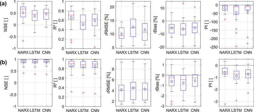
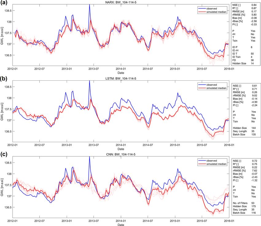
1678                                       A. Wunsch et al.: Groundwater level forecasting with LSTM, CNNs, and NARX

model itself, which needs to be outperformed in the case of        and thus the number of past predicted GWL values available
the PI metric (compare Sect. 2.5). PI values below zero there-     via the feedback connection.
fore basically mean that the output is worse than the input,          In contrast to the above-mentioned well, hardly any sys-
which is, apart from the limited benefit for real applications     tematic pattern can be derived from the choice of input pa-
mentioned above, why we refrain from further discussion of         rameters across all wells that even might have physical im-
the models shown in Fig. 4b.                                       plications for each site. Rather, it is noticeable that certain
   For our analysis, we did not make a preselection of hy-         model types seem to prefer also certain inputs. For example,
drographs that show predominantly natural groundwater dy-          temperature is only selected as input in 5 out of 17 cases for
namics and thus a comparatively strong relationship between        LSTM models and in 2 out of 17 cases for CNN models. Fur-
the available input data and the groundwater level. There-         thermore, rH is always selected for LSTM models except for
fore, even though hydrographs possibly influenced by ad-           two times. In the case of NARX models, there seems to be
ditional factors were examined, we can conclude that the           a lack of systematic behaviour. For more details please see
forecasting approach in general works quite well, and we           Tables S2–S4.
reach, for example, median NSE values of ≥ 0.5 for NARX               Our approach assumes a groundwater dynamic mainly
and CNNs, while LSTMs show a median value only slightly            dominated by meteorological factors. We can assume that all
lower. In terms of robustness against the initialization depen-    three model types are basically capable of modelling ground-
dency of all models (ensemble variability), we clearly ob-         water levels very accurately if all relevant input data can be
serve the highest dependency for NARX, followed by CNN             identified. To exemplarily show the influence of additional
and LSTM, while LSTMs on average perform slightly more             input variables, which, however, are usually not available as
robust than CNNs. Including GWLt−1 lowers the error vari-          input for a forecast or even have insufficient historical data,
ance of the ensemble members, which we used to judge ro-           Fig. 6 illustrates the significantly improved performance af-
bustness in this case, by several orders of magnitude for all      ter including the Rhine water level (W ), which is a large
models. NARX and LSTMs on average now show slightly                streamflow within the study area, using the example of the
lower ensemble variability than CNNs; however, all models          NARX model for well BW_710-256-3, which indeed is lo-
are quite close. A corresponding figure was added (Fig. S69).      cated close to the river. Besides improved performance, we
Furthermore, we also added to the Supplement informa-              also observe lower variability of the ensemble member re-
tion on the results of the hyperparameter optimization (Ta-        sults and thus lower dependency to the model initialization,
bles S2–S4), a table with all error measure values of each         which corresponds also to other time series, where we often
considered hydrograph and model (Table S5), and (accord-           find a smaller influence, the more relevant the input data are.
ing to seq2val) forecasting plots (Figs. S1 to S34 in the Sup-     This also confirms that low accuracy is probably due to insuf-
plement).                                                          ficient input data on a case-by-case basis and not necessarily
   Figure 5 shows exemplarily the forecasting performance          because of an inadequate modelling approach. Similarly, this
of all three models for well BW_104-114-5, where all three         applies also to other wells in our dataset that show unsat-
models consistently achieved good results in terms of accu-        isfying forecasting performance. Examples of this are wells
racy. The NARX model (a) outperforms both LSTM (b) and             in the northern part of the study area (e.g. most wells start-
CNN (c) models and shows very high NSE and R 2 values              ing with HE_. . .), for which our approach is generally more
between 0.8 and 0.9. The CNN model provides the second             challenging due to strong groundwater extraction activities
best forecast, which even very slightly shows less underesti-      in this area, as well as well BW_138-019-0, which is close
mation (Bias/rBias) of the GWLs than the NARX model. By            to the Rhine and probably under the influence of a large ship
comparing the graphs in (a) and (c), we assume that this is        lock nearby. Additionally, this well is within a flood retention
only true on average. The CNN model overestimates in 2012          area that is spatially coupled to the ship lock.
and constantly underestimates the last third of the test period.
The NARX model, however, is more consistent and there-             4.2   Sequence-to-sequence (seq2seq) forecasting
fore better. Concerning R 2 values, the LSTM basically keeps             performance
up with the CNN, and all other error measures show the
still good (but in comparison worst) values. We notice that        Sequence-to-sequence forecasting is especially interesting
in accordance to our overall findings mentioned above, the         for short- and mid-term forecasts, because the input variables
LSTM shows the lowest ensemble variability and therefore           only have to be available until the start of the forecast. Fig-
the smallest initialization dependency. Taking a look at the       ure 7 summarizes and compares the overall seq2seq forecast-
selected inputs and hyperparameters, we notice that relative       ing accuracy of the three model types for all 17 wells. Fig-
humidity (rH) does not seem to provide important informa-          ure 7a shows the performance when only meteorological in-
tion and was therefore never selected as an input. Further, the    puts are used; the models in Fig. 7b are additionally provided
input sequence length of both LSTM and CNN is equally 35           with GWLt−1 as an input. Similarly to the seq2val forecasts
steps (weeks). In the NARX model there is no direct corre-         (Fig. 4), past GWLs seem to be especially important for
spondence, but a similar value is shown by the parameter FD        LSTM and CNN models, where this additional input vari-

Hydrol. Earth Syst. Sci., 25, 1671–1687, 2021                                       https://doi.org/10.5194/hess-25-1671-2021
A. Wunsch et al.: Groundwater level forecasting with LSTM, CNNs, and NARX                                                     1679

Figure 5. Forecasts of (a) a NARX, (b) a LSTM and (c) a CNN model for well BW_104-114-5 during the test period 2012–2016.

able causes substantial performance improvement. Without            world applications. Detailed results on all seq2seq models
past GWLs, NARX seem to be clearly superior due to their            can be found Table S6 and Figs. S35 to S68.
inherent global feedback connection. However, NARX show                Figure 8 summarizes exemplarily for well HE_11874
almost equal performance values in both scenarios (Fig. 7a          the sequence-to-sequence forecasting performance for
and b). In contrast to the seq2val forecasts, NARX system-          NARX (a, b), LSTMs (c, d), CNNs (e, f), only with meteo-
atically show lower R 2 values than LSTM and CNN mod-               rological input variables (a, c, e), and with an additional past
els for seq2seq forecasts. For all other error measures, the        GWL input (b, d, f). These confirm that GWLt−1 substan-
accuracy of NARX models outperforms LSTMs and CNNs                  tially improves the performance of LSTMs and CNNs; how-
in a direct comparison for the vast majority of all time se-        ever, NARX forecasts in this case only improve very slightly.
ries. While LSTMs and CNNs show lower performance for               Especially for LSTMs and CNNs, it is easily visible that the
sequence-to-sequence forecasting compared to sequence-to-           sequence forecasts of the better models (d,f) mostly estimate
value forecasting, NARX seq2seq models even outperform              the intensity of a future groundwater level change too con-
NARX seq2val models (except for R 2 ). This is quite counter-       servatively; thus, both increases and decreases are predicted
intuitive as one would expect it to be more difficult to forecast   too weak. This is a commonly known issue with ANNs, as
a whole sequence than a single value. All in all, the scenario      extreme values are typically underrepresented in the distri-
including past GWLs (Fig. 7b) seems to be the preferable one        bution of the training data (e.g. Sudheer et al., 2003). We fur-
for all three models and shows promising results for real-          ther notice that the robustness of LSTMs and CNNs in terms
                                                                    of initialization dependency and thus the ensemble variabil-

https://doi.org/10.5194/hess-25-1671-2021                                        Hydrol. Earth Syst. Sci., 25, 1671–1687, 2021
1680 A. Wunsch et al.: Groundwater level forecasting with LSTM, CNNs, and NARX Figure 6. Forecasting performance exemplarily shown for NARX model of well BW_710-256-3 (a) based on meteorological input variables and (b) improved performance after including the Rhine water level (W ) as input variable. Figure 7. Boxplots showing the seq2seq forecast accuracy of NARX, LSTM, and CNN models within the test period (2012–2016) for all considered 17 hydrographs. The diamond symbols indicate the arithmetic mean; (a) only meteorological inputs; (b) GWLt−1 as additional input. ity significantly improves when past GWLs are provided as fore should not be evaluated without including an initializa- inputs (Fig. 8). This is also supported by analysing the en- tion ensemble. The initialization dependency of LSTMs and semble member error variances and also true for all other CNNs is significantly lower, with LSTMs being even more time series in the dataset as well (Fig. S69). Just like for robust than CNNs. seq2val forecasts, NARX usually show a significantly lower The extraordinary performance of the NARX models, es- robustness in terms of initialization dependency; however, pecially in the case of well HE_11874 (Fig. 8) is surpris- the median ensemble performance nevertheless is of high ing, because the performance substantially outperforms the accuracy. All models, but especially NARX models, there- seq2val NARX without GWLt−1 input (e.g. NSE: 0.35, Hydrol. Earth Syst. Sci., 25, 1671–1687, 2021 https://doi.org/10.5194/hess-25-1671-2021
A. Wunsch et al.: Groundwater level forecasting with LSTM, CNNs, and NARX                                                   1681

R 2 : 0.75); however, the seq2val NARX model with GWLt−1          4.4   Influence of training data length
inputs also showed high accuracy (e.g. NSE: 0.99, R 2 : 0.99).
It is also interesting to note that the sequence predictions      In the following section we explore similarities and differ-
of the NARX models overlap exactly, and the individual se-        ences of NARX, LSTMs, and CNNs in terms of the influ-
quences are therefore no longer visible. One reason for this      ence of training data length. It is commonly known that data-
different behaviour compared to the LSTM and CNN models           driven approaches profit from additional data; however, how
is probably that the technical approach for seq2seq forecast-     much data are necessary to build models that are able to per-
ing differs for these models. While LSTMs and CNNs use            form reasonable calculations still remains an open question.
multiple output neurons to predict multiple time steps, this      This is because the answer is highly dependent on the ap-
approach for us did not yield meaningful results for a NARX       plication case, data properties (e.g. distribution), and model
model, probably because of feedback connection issues. In-        properties, as model depth can sometimes exponentially de-
stead we used one NARX output neuron to predict a multi-          crease the need for training data (Goodfellow et al., 2016).
element vector at once.                                           Therefore, this question cannot be entirely answered by a
                                                                  simple analysis like we perform here. Nevertheless, we still
4.3   Hyperparameter optimization and computational               want to give an impression of how much data might be ap-
      aspects                                                     proximately needed in the case of groundwater level data
                                                                  in porous aquifers and if the models substantially differ in
During the HP optimization, depending on the forecasting          their need for training data. For our analysis, we always
approach (seq2val/seq2seq) and available inputs (with or          consider the forecasting accuracy during the 4-year testing
without GWLt−1 ), there were noticeable differences with re-      period (2012–2016) and systematically expand the training
gard to the number of iterations required and the associated      data basis year by year, starting in 2010, thus with only
time needed (Fig. 9). The best parameter combination, es-         clearly insufficient 2 years of training data. We focus on
pecially for CNN and LSTM networks, was often found in            sequence-to-value forecasting due to the easier interpretabil-
33 steps or fewer, i.e. after 25 obligatory random exploration    ity of the results, and we always consider the median per-
steps in only 8 Bayesian steps. Please note that prior to the     formance of 10 different model initializations for evaluation.
analysis we chose to at least perform 50 optimization steps,      Figure 10 summarizes the performance and the improve-
which explains the distribution in the “total iterations” col-    ment that comes with additional training data; all values are
umn. In column two (“best iteration”) we can observe simi-        normalized per well to make them comparable. Please note
lar behaviour of CNNs and LSTMs, while NARX are always            that all models at least show 28 years of training data (un-
somehow different to these two. We suspect that this is rather    til 1982), and only three models exceed 30 years of train-
an influence of the software or the optimization algorithm,       ing data (1980); thus, the number of samples represented by
since especially model types implemented in Python show           the boxplots decreases significantly after 30 years. Figure 10
an identical behaviour. However, in the majority of cases         summarizes as well models with and without GWLt−1 in-
the best iteration was found in less than 33 steps; the mini-     puts, because no significantly different behaviour was ob-
mum as well as the maximum number of iteration steps were         served for each group. Please find corresponding figures for
therefore obviously sufficient. It is interesting that for CNNs   each group in Figs. S70 and S71.
and LSTM the number of steps is similar throughout the               As expected, we observe significant improvements with
experiments, whereas for NARX the inclusion of GWLt−1             additional training data. NARX models seem to improve
as input caused an increase in iterations. Columns three to       more or less continuously and also work better with few data,
five in Fig. 9 show substantial differences concerning the        whereas for LSTMs and CNNs some kind of threshold is vis-
calculation speed of the three model types. CNNs outper-          ible (about 10 years, thus approx. 500 samples), where the
form all other models systematically; however, concerning         performance significantly increases and rapidly approaches
the sequence-to-sequence forecasts, NARX models can al-           the optimum. It should be noted, though, that this can proba-
most keep up. We also observe that LSTMs seem to slow             bly not be transferred to other time steps; that is, in the case
down when including GWLt−1 as input or when performing            of daily values, 500 d will most certainly not be enough, since
seq2seq forecasts, the opposite happens in the case of NARX       only one full yearly cycle is included. We explored the reason
models, which speed up in these cases. This also means that       for this threshold and observed that when stopping the train-
even though NARX models need more optimization itera-             ing 5 years earlier (2007), the threshold now occurs corre-
tions until the assumed optimum than LSTMs, in terms of           spondingly 5 years earlier (Fig. S72). Additionally, we found
time they outperform them due to shorter duration per iter-       that several standard statistic values such as mean; median;
ation (column 3). Please note that it is out of the scope of      variance; overall maximum; and the percentiles at 25, 75, and
this work to provide detailed assessments of the calculation      97.5 show similar thresholds (Fig. S73). Thus, the early years
speed under benchmark conditions, but we do share practical       of the 2000s seem to be especially relevant for our test pe-
insights for fellow hydrogeologists.                              riod. This is a highly dataset-specific observation that can-
                                                                  not be generalized; however, this also shows that it is vital

https://doi.org/10.5194/hess-25-1671-2021                                      Hydrol. Earth Syst. Sci., 25, 1671–1687, 2021
1682 A. Wunsch et al.: Groundwater level forecasting with LSTM, CNNs, and NARX Figure 8. Forecasts of (a, b) a NARX, (c, d) a LSTM, and (e, f) a CNN model for well BW_104-114-5 during the test period 2012–2016. Models in (a, c, e) use only meteorological input variables, and models in (b, d, f) use also past GWL observations. Hydrol. Earth Syst. Sci., 25, 1671–1687, 2021 https://doi.org/10.5194/hess-25-1671-2021
A. Wunsch et al.: Groundwater level forecasting with LSTM, CNNs, and NARX                                                            1683

Figure 9. Comparison of the performed HP optimizations (columns 1 and 2); their calculation time per iteration in seconds (column 3), until
the optimum was found (minutes) (column 4); and the total time spent on optimization in hours (column 5).

Figure 10. Influence of training data length on model performance.

https://doi.org/10.5194/hess-25-1671-2021                                             Hydrol. Earth Syst. Sci., 25, 1671–1687, 2021
1684                                      A. Wunsch et al.: Groundwater level forecasting with LSTM, CNNs, and NARX

to include relevant training data, which is, however, not very       The results are surprising in a way that LSTMs are widely
easy to identify. Nevertheless as a rule of thumb the chance      known to perform especially well on sequential data and are
of using the right data increases with the amount of avail-       therefore also more commonly applied. In this work they
able data. These findings are supported by the observation        were outperformed by CNNs and NARX models. We showed
that not every additional year improves the accuracy; only the    that for this specific application (i) CNNs might be the bet-
overall trend is positive. This seems plausible, because espe-    ter choice due to significantly faster calculation and mostly
cially when conditions change over time, the models can also      similar performance, and (ii) even though DL approaches
learn behaviour that is no longer valid and which possibly        are currently often preferred over traditional (shallow) neural
decreases future forecast performance. One should therefore       networks such as NARX, the latter should not be neglected
not only include as much data as possible but also carefully      in the selection processes especially when there is few train-
evaluate and also possibly shorten the training database if       ing data available. Particularly NARX sequence-to-sequence
necessary.                                                        forecasting seems to be promising for short- and mid-term
                                                                  forecasts. However, we do not want to ignore the fact that
                                                                  LSTMs and CNNs might perform substantially better with
5   Conclusions                                                   a larger dataset, which better fulfils common definitions of
                                                                  DL applications and where deeper networks can demonstrate
In this study we evaluate and compare the groundwater level
                                                                  their strengths, such as automated feature extraction. Since
forecasting accuracy of NARX, CNN and LSTM models. We
                                                                  such data are usually not available in groundwater level pre-
examine sequence-to-value and sequence-to-sequence fore-
                                                                  diction tasks yet, for the moment this remains in theory.
casting scenarios. We can conclude that in the case of seq2val
forecasts all models are able to produce satisfying results,
and NARX models on average perform best, while LSTMs              Code and data availability. All groundwater data are available for
perform the worst. Since CNNs are much faster in calcula-         free via the web services of the local authorities (HLNUG, 2019;
tion speed than NARX and only slightly behind in terms of         LUBW, 2018; MUEEF, 2018). Meteorological input data was de-
accuracy, they might be the favourable option if time is an is-   rived from the HYRAS dataset (Frick et al., 2014; Rauthe et al.,
sue. If accuracy is especially important, one should stick with   2013), which can be obtained free of charge for non-commercial
NARX models. LSTMs, however, are most robust against              purposes on request from the German Meteorological Service
initialization effects, especially compared to NARX. Includ-      (DWD, 2021). Our Python and MATLAB code files are available
ing past groundwater levels as inputs strongly improves CNN       on GitHub (Wunsch, 2020).
and LSTM seq2val forecast accuracy. However, all three
models mostly cannot beat the naïve model in this scenario
and are therefore of no value.                                    Supplement. The supplement related to this article is available on-
   Especially when no input data are available in short- and      line at: https://doi.org/10.5194/hess-25-1671-2021-supplement.
mid-term forecasting applications, sequence-to-sequence
forecasting is of special interest. Again, past groundwater
                                                                  Author contributions. AW conceptualized the study, wrote the
levels as input significantly improved CNN and LSTM per-
                                                                  code, validated and visualized the results, and wrote the original
formance, while NARX performed almost similar in both
                                                                  paper draft. All three authors contributed to the methodology and
scenarios. Overall, NARX models show the best perfor-             performed review and editing tasks. TL contributed to the concep-
mance (except R 2 values) in the vast majority of all cases. In   tualization and validation as well and further supervised the work.
addition to the fast calculation of NARX in this case, which
almost keeps up with CNN speed, they are clearly prefer-
able. However, NARX models are least robust against ini-          Competing interests. The authors declare that they have no conflict
tialization effects, which nevertheless are easy to handle by     of interest.
implementing a forecasting ensemble.
   We further analysed what data might be needed or suffi-
cient to reach acceptable results. As expected, we found that     Financial support. The article processing charges for this open-
in principle the longer the training data, the better; however,   access publication were covered by a Research Centre of the
a noteworthy threshold seems to exist for about 10 years          Helmholtz Association.
of weekly training data, below which the performance be-
comes significantly worse. This applies especially for LSTM
and CNN models but was also found to probably be highly           Review statement. This paper was edited by Mauro Giudici and re-
dataset specific. Overall, NARX seem to perform better in         viewed by Daniel Klotz and one anonymous referee.
comparison to CNN and LSTM models, when only few train-
ing data are available.

Hydrol. Earth Syst. Sci., 25, 1671–1687, 2021                                       https://doi.org/10.5194/hess-25-1671-2021
A. Wunsch et al.: Groundwater level forecasting with LSTM, CNNs, and NARX 1685
References Deep Learning, IEEE Trans. Geosci. Remote, 57, 2221–2233,
https://doi.org/10.1109/TGRS.2018.2872131, 2019.
Fang, K., Kifer, D., Lawson, K., and Shen, C.: Evaluating
Abadi, M., Agarwal, A., Barham, P., Brevdo, E., Chen, Z., Citro, the Potential and Challenges of an Uncertainty Quantification
C., Corrado, G. S., Davis, A., Dean, J., Devin, M., Ghemawat, S., Method for Long Short-Term Memory Models for Soil Mois-
Goodfellow, I., Harp, A., Irving, G., Isard, M., Jia, Y., Jozefow- ture Predictions, Water Resour. Res., 56, e2020WR028095,
icz, R., Kaiser, L., Kudlur, M., Levenberg, J., Mane, D., Monga, https://doi.org/10.1029/2020WR028095, 2020.
R., Moore, S., Murray, D., Olah, C., Schuster, M., Shlens, J., FAO: The Wealth of Waste: The Economics of Wastewater Use in
Steiner, B., Sutskever, I., Talwar, K., Tucker, P., Vanhoucke, Agriculture, no. 35 in FAO Water Reports, Food and Agriculture
V., Vasudevan, V., Viegas, F., Vinyals, O., Warden, P., Wat- Organization of the United Nations, Rome, 2010.
tenberg, M., Wicke, M., Yu, Y., and Zheng, X.: TensorFlow: Frick, C., Steiner, H., Mazurkiewicz, A., Riediger, U., Rauthe,
Large-Scale Machine Learning on Heterogeneous Distributed M., Reich, T., and Gratzki, A.: Central European High-
Systems, p. 19, available at: https://www.tensorflow.org/ (last ac- Resolution Gridded Daily Data Sets (HYRAS): Mean Tem-
cess: 30 March 2021), 2015. perature and Relative Humidity, Meteorol. Z., 23, 15–32,
Adamowski, J. and Chan, H. F.: A Wavelet Neural Network Con- https://doi.org/10.1127/0941-2948/2014/0560, 2014.
junction Model for Groundwater Level Forecasting, J. Hydrol., Gauch, M., Kratzert, F., Klotz, D., Nearing, G., Lin, J., and Hochre-
407, 28–40, https://doi.org/10.1016/j.jhydrol.2011.06.013, 2011. iter, S.: Rainfall–Runoff Prediction at Multiple Timescales with
Afzaal, H., Farooque, A. A., Abbas, F., Acharya, B., and Esau, T.: a Single Long Short-Term Memory Network, Hydrol. Earth Syst.
Groundwater Estimation from Major Physical Hydrology Com- Sci. Discuss. [preprint], https://doi.org/10.5194/hess-2020-540,
ponents Using Artificial Neural Networks and Deep Learning, in review, 2020.
Water, 12, 5, https://doi.org/10.3390/w12010005, 2020. Gauch, M., Mai, J., and Lin, J.: The Proper Care and
Alsumaiei, A. A.: A Nonlinear Autoregressive Modeling Ap- Feeding of CAMELS: How Limited Training Data Affects
proach for Forecasting Groundwater Level Fluctuation in Urban Streamflow Prediction, Environ. Model. Softw., 135, 104926,
Aquifers, Water, 12, 820, https://doi.org/10.3390/w12030820, https://doi.org/10.1016/j.envsoft.2020.104926, 2021.
2020. Gers, F. A., Schmidhuber, J., and Cummins, F.: Learning to Forget:
Beale, H. M., Hagan, M. T., and Demuth, H. B.: Neural Net- Continual Prediction with LSTM, Neural Comput., 12, 2451–
work ToolboxTM User’s Guide: Revised for Version 9.1 (Re- 2471, https://doi.org/10.1162/089976600300015015, 2000.
lease 2016b), The MathWorks, Inc., available at: https://de. Goodfellow, I., Bengio, Y., and Courville, A.: Deep Learning,
mathworks.com/help/releases/R2016b/nnet/index.html (last ac- Adaptive Computation and Machine Learning, The MIT Press,
cess: 30 March 2021), 2016. Cambridge, Massachusetts, 2016.
Bengio, Y., Simard, P., and Frasconi, P.: Learning Long-Term De- Guzman, S. M., Paz, J. O., and Tagert, M. L. M.: The Use
pendencies with Gradient Descent Is Difficult, IEEE Trans. Neu- of NARX Neural Networks to Forecast Daily Ground-
ral Netw., 5, 157–166, https://doi.org/10.1109/72.279181, 1994. water Levels, Water Resour. Manage., 31, 1591–1603,
Bowes, B. D., Sadler, J. M., Morsy, M. M., Behl, M., and Goodall, https://doi.org/10.1007/s11269-017-1598-5, 2017.
J. L.: Forecasting Groundwater Table in a Flood Prone Coastal Guzman, S. M., Paz, J. O., Tagert, M. L. M., and Mercer,
City with Long Short-Term Memory and Recurrent Neural A. E.: Evaluation of Seasonally Classified Inputs for the Pre-
Networks, Water, 11, 1098, https://doi.org/10.3390/w11051098, diction of Daily Groundwater Levels: NARX Networks Vs Sup-
2019. port Vector Machines, Environ. Model. Assess., 24, 223–234,
Chang, F.-J., Chang, L.-C., Huang, C.-W., and Kao, I.-F.: Pre- https://doi.org/10.1007/s10666-018-9639-x, 2019.
diction of Monthly Regional Groundwater Levels through Hy- Hasda, R., Rahaman, M. F., Jahan, C. S., Molla, K. I., and
brid Soft-Computing Techniques, J. Hydrol., 541, 965–976, Mazumder, Q. H.: Climatic Data Analysis for Ground-
https://doi.org/10.1016/j.jhydrol.2016.08.006, 2016. water Level Simulation in Drought Prone Barind Tract,
Chen, Y., Kang, Y., Chen, Y., and Wang, Z.: Prob- Bangladesh: Modelling Approach Using Artificial Neu-
abilistic Forecasting with Temporal Convolutional ral Network, Groundwater Sustain. Dev., 10, 100361,
Neural Network, Neurocomputing, 399, 491–501, https://doi.org/10.1016/j.gsd.2020.100361, 2020.
https://doi.org/10.1016/j.neucom.2020.03.011, 2020. HLNUG: GruSchu, available at: http://gruschu.hessen.de (last ac-
Chollet, F.: Keras, Keras, GitHub, available at: https://github.com/ cess: 30 March 2021), 2019.
fchollet/keras (last access: 30 March 2021), 2015. Hochreiter, S. and Schmidhuber, J.: Long Short-
Di Nunno, F. and Granata, F.: Groundwater Level Pre- Term Memory, Neural Comput., 9, 1735–1780,
diction in Apulia Region (Southern Italy) Using https://doi.org/10.1162/neco.1997.9.8.1735, 1997.
NARX Neural Network, Environ. Res., 190, 110062, Hunter, J. D.: Matplotlib: A 2D Graphics Environment, Com-
https://doi.org/10.1016/j.envres.2020.110062, 2020. put. Sci. Eng., 9, 90–95, https://doi.org/10.1109/MCSE.2007.55,
Duan, S., Ullrich, P., and Shu, L.: Using Convolutional Neural Net- 2007.
works for Streamflow Projection in California, Front. Water, 2, Izady, A., Davary, K., Alizadeh, A., Moghaddamnia, A., Zi-
28, https://doi.org/10.3389/frwa.2020.00028, 2020. aei, A. N., and Hasheminia, S. M.: Application of NN-
DWD: HYRAS – Hydrologische Rasterdatensätze, available ARX Model to Predict Groundwater Levels in the Neisha-
at: https://www.dwd.de/DE/leistungen/hyras/hyras.html, last ac- boor Plain, Iran, Water Resour. Manage., 27, 4773–4794,
cess: 30 March 2021. https://doi.org/10.1007/s11269-013-0432-y, 2013.
Fang, K., Pan, M., and Shen, C.: The Value of SMAP
for Long-Term Soil Moisture Estimation With the Help of
https://doi.org/10.5194/hess-25-1671-2021 Hydrol. Earth Syst. Sci., 25, 1671–1687, 2021You can also read