PYRATES - A PYTHON FRAMEWORK FOR RATE-BASED NEURAL SIMULATIONS - BIORXIV
←
→
Page content transcription
If your browser does not render page correctly, please read the page content below
bioRxiv preprint first posted online Apr. 13, 2019; doi: http://dx.doi.org/10.1101/608067. The copyright holder for this preprint
(which was not peer-reviewed) is the author/funder, who has granted bioRxiv a license to display the preprint in perpetuity.
                                  It is made available under a CC-BY 4.0 International license.

               PyRates - A Python Framework for Rate-Based Neural Simulations

                   Richard Gast and Daniel Rose, Harald E. Möller, Nikolaus Weiskopf, Thomas R. Knösche
                                   Max-Planck-Institute for Human Cognitive and Brain Sciences, Leipzig, Germany

   Abstract
   In neuroscience, computational modeling has become an important source of insight into brain states and dynamics.
   A basic requirement for computational modeling studies is the availability of efficient software for setting up models
   and performing numerical simulations. While many such tools exist for different families of neural models, there is
   a lack of tools allowing for both a generic model definition and efficiently parallelized simulations. In this work, we
   present PyRates, a Python framework that provides the means to build a large variety of neural models as a graph.
   PyRates provides intuitive access to and modification of all mathematical operators in a graph, thus allowing for
   a highly generic model definition. For computational efficiency and parallelization, the model graph is translated
   into a tensorflow-based compute graph. Using the example of two different neural models belonging to the family
   of rate-based population models, we explain the mathematical formalism, software structure and user interfaces of
   PyRates. We then show via numerical simulations that the behavior shown by the model implementations in PyRates
   is consistent with the literature. Finally, we demonstrate the computational capacities and scalability of PyRates via a
   number of benchmark simulations of neural networks differing in size and connectivity.
   Keywords: PyRates, neural models, simulation software, tensorflow, computational modeling, parallelization

   1. Introduction
        In the last decades, computational neuroscience has become an integral part of neuroscientific research. A major
   factor in this development has been the difficulty to gain mechanistic insights into neural processes and structures from
   recordings of brain activity without additional computational models. This problem is strongly connected to the sig-
   nals recorded with non-invasive brain imaging techniques such as magneto- and electroencephalography (MEG/EEG)
   or functional magnetic resonance imaging (fMRI). Even though the spatiotemporal resolution of these techniques has
   improved throughout the years, they are still limited with respect to the state variables of the brain they can pick up.
   Spatial resolution in fMRI has been pushed to the sub-millimeter range [1, 2], whereas EEG and MEG offer a temporal
   resolution thought to be sufficient to capture all major signaling processes in the brain [3]. On the EEG/MEG side, the
   measured signal is thought to arise mainly from the superposition of primary and secondary currents resulting from
   post-synaptic polarization of a large number of cells with similarly oriented dendrites [4]. Therefore, the activity of
   cell-types that do not show a clear orientation preference (like most inhibitory interneurons [5]) can barely be picked
   up, even though they might play a crucial role for the underlying neural dynamics. Further issues of EEG/MEG acqui-
   sitions are their limited sensitivity to sub-cortical signal sources and the inverse problem one is facing when trying to
   locate the source of a signal within the brain [6]. On the other hand, fMRI measures hemodynamic signals of the brain
   related to local blood flow, blood volume and blood oxygenation levels and thus delivers only an indirect, strongly
   blurred view on the dynamic state of the brain [7]. These limitations pose the need for additional models and assump-
   tions that link the recorded signals to the underlying neural activity. Computational models of brain dynamics (called
   neural models henceforth) are therefore particularly important for interpreting neuroimaging data and understanding
   the neural mechanisms involved in their generation [8, 9, 10]. Such models have been developed for various spatial
   and temporal scales of the brain, ranging from highly detailed models of a single neuron to models that represent the
   lumped activity of thousands of neurons. In any case, they provide observation and control over all state variables
   included in a given model, thus offering mechanistic insights into their dynamics.
        Numerical simulations are the major method used to investigate neural models beyond pure mathematical analyses
   and link model variables to experimental data. Such numerical simulations can be computationally highly expensive
   Preprint submitted to bioRxiv                                                                                              April 12, 2019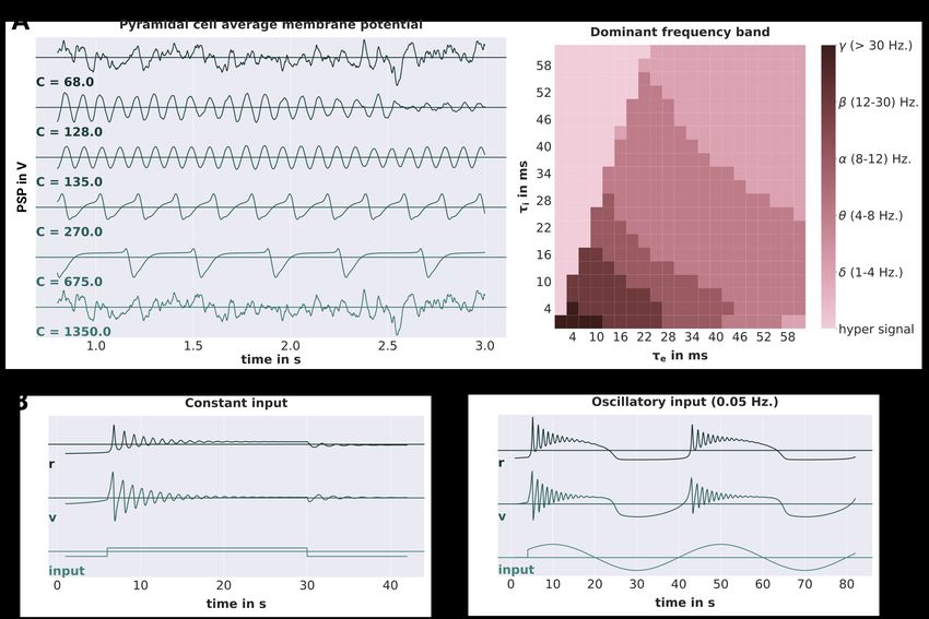
bioRxiv preprint first posted online Apr. 13, 2019; doi: http://dx.doi.org/10.1101/608067. The copyright holder for this preprint
(which was not peer-reviewed) is the author/funder, who has granted bioRxiv a license to display the preprint in perpetuity.
                                  It is made available under a CC-BY 4.0 International license.

   and scale with the model size, simulation time and temporal resolution of the simulation. Different software tools have
   been developed for neural modeling that offer various solutions to render numerical simulations more efficient (e.g.
   TVB [11], DCM [12], Nengo [13], NEST [14], ANNarchy [15], Brian [16], NEURON [17]). Since the brain is an
   inherently highly parallelized information processing system (i.e. all of its 10 billion neurons transform and propagate
   signals in parallel), most models of the brain have a high degree of structural parallelism as well. This means that
   they involve calculations that can be evaluated in parallel, as for example the update of the firing rate of each cell
   population inside a neural model. One obvious way of optimizing numerical simulations of neural models is therefore
   to distribute these calculations on the parallel hardware of a computer, i.e. its central and graphical processing units
   (CPUs and GPUs). Neural simulation tools that implement such mechanisms include ANNarchy [15], Brian [16],
   NEURON [18], Nengo [13] and PCSIM [19], for example. Each of these tools has been build for neural models of a
   certain family. While complex multi-compartment models of single spiking neurons are implemented in NEURON,
   models of point neurons are provided by ANNarchy, Brain, Nengo, Nest and PCSIM, whereas neural population
   models are found in TVB and DCM. For most of these tools, a pool of pre-implemented models of the given family
   are available that the user can choose from. However, most often it is not possible to add new models or modeling
   mechanisms to this pool without considerable effort. This holds true especially, if one still wants to benefit from the
   parallelization and optimization features of the respective software. Exceptions are tools like ANNarchy and Brian
   that include code generation mechanisms. These allow the user to define the mathematical equations that certain
   parts of the model will be governed by and will automatically translate them into the same representations that the
   pre-implemented models follow. Unfortunately, the tools that provide such code generation mechanisms are limited
   with regards to the model parts they allow to be customized in such a way and the families of neural models they can
   express.
       To summarize, we believe that the increasing number of computational models and numerical simulations in
   neuroscientific research motivates the development of neural simulation tools that:

       • follow a well-defined mathematical formalism in their model configurations,
       • are flexible enough so scientists can implement custom models that go beyond pre-implemented models in both
         the mathematical equations and network structure,
       • are structured in a way such that models are easily understood, set up and shared with other scientists,
       • enable efficient numerical simulations on parallel computing hardware.

       In this work, we present PyRates, a Python framework which is in line with these suggestions (available from
   https://github.com/pyrates-neuroscience/PyRates). The basic idea behind PyRates is to provide a well
   documented, thoroughly tested and computationally powerful framework for neural modeling and simulations.
   Thereby, our solution to the parallelization issue is to translate every model implemented in PyRates into a tensorflow
   [20] graph, a powerful compute engine that provides efficient CPU and GPU parallelization. We will provide a more
   detailed description of this feature in Section 3. Each model in PyRates is represented by a graph of nodes and edges,
   with the former representing the model units (i.e. single cells, cell populations, ...) and the latter the information
   transfer between them. As we will explain in more detail in Section 3, the user has full control over the mathematical
   equations that nodes and edges are defined by. Still, both the model configuration and simulation can be done within
   a few lines of code. In principle, this allows to implement any kind of dynamic neural system that can be expressed
   as a graph. However, for the remainder of this article, we will focus on a specific family of neural models, namely
   rate-based population models (hence the name PyRates), which will be introduced in the next section. The focus on
   population models is (i) in accordance with the expertise of the authors and (ii) serves the purpose of keeping the
   article concise. However, even though neural population models were chosen as exemplary models, the emphasize
   of the paper lies on introducing the features and capacities of the framework, how to define a model in PyRates and
   how to use the software to perform and analyze neural simulations. In Section 3, we first introduce the mathematical
   syntax used for all our models, followed by an explanation how single mathematical equations are structured in
   PyRates to form a neural network model. To this end, we provide a step-by-step example of how to configure and
   simulate a particular neural population model. We continue with a section dedicated to the evaluation of different
   numerical simulation scenarios. First, we validate the implementation of two exemplary neural population models in

                                                                       2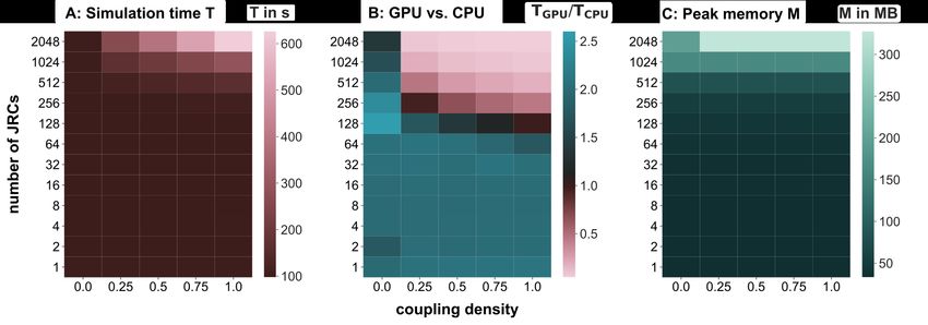
bioRxiv preprint first posted online Apr. 13, 2019; doi: http://dx.doi.org/10.1101/608067. The copyright holder for this preprint
(which was not peer-reviewed) is the author/funder, who has granted bioRxiv a license to display the preprint in perpetuity.
                                  It is made available under a CC-BY 4.0 International license.

   PyRates by replicating key behaviors of the models reported in their original publications. Second, we demonstrate
   the computational efficiency and scalability of PyRates via a number of benchmarks. These benchmarks constitute
   different realistic test networks that differ in size and sparseness of their connectivity. Furthermore, we discuss the
   strengths and limitations of PyRates for developing and simulating neural models.

   2. Neural Population Models
        Investigating the human brain via EEG/MEG or fMRI means working with signals that are assumed to represent
   changes in the average activity of large cell populations. While these signals could in theory be explained by detailed
   models of single cell processes, such models come with a state space of much higher dimensionality than the measured
   signals and would thus need to be reduced again for comparison. Additionally, the interpretability of single cell
   activities would be limited, since an average signal is modelled that could result from endlessly many different single
   cell activation patterns. As an alternative, neural population models (also called neural mass models) have widely
   been used [21]. They are biophysically motivated non-linear models of neural dynamics that describe the average
   activity of large cell populations in the brain via a mean-field approach [22, 23, 24]. Often, they express the state
   of each neural population by an average membrane potential and an average firing rate. This allows for a more
   direct comparison to EEG/MEG and fMRI signals, since the changes in the average activity across many cells are
   thought to generate those signals [25, 26]. The dynamics and transformations of these state variables can typically be
   formulated via three mathematical operators. The first two describe the input-output structure of a single population:
   While the rate-to-potential operator (RPO) transforms synaptic inputs into average membrane potential changes, the
   potential-to-rate operator (PRO) transforms the average membrane potential into an average firing rate output. Widely
   used forms for these operators are a convolution operation with an alpha kernel for the RPO (e.g. [24, 25, 27])
   and a sigmoidal, instantaneous transformation for the PRO (e.g. [23, 28, 29]). The third operator is the coupling
   operator (CO) that transforms outgoing into incoming firing rates and is thus used to establish connections across
   populations. By describing the dynamics of large neural population networks via three basic transforms (RPO, PRO
   & CO), neural populations combine computational feasibility with biophysical interpretability. Due to these desirable
   qualities, they have become an attractive method for studying neural dynamics on a meso- and macroscopic scale
   [8, 21, 10]. They have been established as one of the most popular methods for modeling EEG/MEG and fMRI
   measurements and were able to account for various dynamic properties of experimentally observed neural activity
   [30, 26, 31, 32, 27, 33, 34, 35].
        A particular neural population model we will use repeatedly in later sections is the three-population circuit intro-
   duced by Jansen and Rit [24]. The Jansen-Rit circuit (JRC) was originally proposed as a mechanistic model of the
   EEG signal generated by the visual cortex [36, 24]. Historically, however, it has been used as a canonical model of cell
   population interactions in a cortical column [30, 31, 35]. Its basic structure can be seen in Figure 1 B, which can be
   thought of as a zoom-in on a single cortical column. The signal generated by this column is the result of the dynamic
   interactions between a projection cell population (PC), an excitatory interneuron population (EIN) and an inhibitory
   interneuron population (IIN). For certain parametrizations, the JRC has been shown to be able to produce key features
   of a typical EEG signal, such as the waxing-and-waning alpha oscillations [24, 25, 37]. A detailed account of the
   model’s mathematical description will be given in the next section, where we will demonstrate how to implement
   models in PyRates, using the example of the JRC equations. We chose to employ the JRC as an exemplary population
   model in this article, since it is an established model used in numerous publications the reader can compare our reports
   against.
        Another neural population model that we will make use of in this paper is the one described by Montbrió et al.
   [38]. It has been mentioned as one of the next generation neural mass models that provide a more precise mean-field
   description than classic neural population models like the JRC [39]. The model proposed by Montbrió et al. represents
   a mathematically exact mean-field derivation of a network of globally coupled quadratic integrate-and-fire neurons
   [38]. It can thus represent every macroscopic state the single cell network may fall into. This distinguishes it from the
   JRC, since it has no such correspondence between a single cell network and the population descriptions. Furthermore,
   the macroscopic states (average membrane potential and average firing rate) of the Montbrió model can be linked
   directly to the synchronicity of the underlying single-cell network, a property which benefits the investigation of
   EEG phenomena such as event-related (de-)synchronization. We chose this model as our second example case due to
   its novelty and its potential importance for future neural population studies. Within the domain of rate-based neural
                                                                       3
bioRxiv preprint first posted online Apr. 13, 2019; doi: http://dx.doi.org/10.1101/608067. The copyright holder for this preprint
(which was not peer-reviewed) is the author/funder, who has granted bioRxiv a license to display the preprint in perpetuity.
It is made available under a CC-BY 4.0 International license.
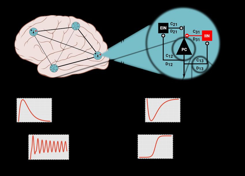
Figure 1: Model structure in PyRates. The largest organisational unit of a network model is the Circuit. Any circuit may
also consist of multiple hierarchical layers of subcircuits. Panel (A) depicts an imaginary circuit that encompasses four
subcircuits that represent one brain region each. One of these local circuits is a Jansen-Rit circuit (B), consisting of three
neural populations (PC, EIN, IIN) and connections between them. One node (C) may consist of multiple operators that
contain the mathematical equations. Here, two rate-to-potential operators (RPO) convolute incoming firing rates with an
alpha kernel to produce post-synaptic potentials. These are summarized int a mean membrane potential V. The
potential-to-rate operator (PRO) transforms V into outgoing firing rate mo ut via a sigmoid function. Inset graphs give a
qualitative representation of the operators and evolution of the membrane potential. Edges (lines in A and B) represent
information transfer between nodes. As panel (D) shows, edges may also contain operators. By default, edges apply a
multiplicative weighting constant and can optionally delay the information passage with respect to time. The equation
shown in panel (D) depicts this default behaviour.
population models, we found these two models sufficiently distinct to demonstrate the ability of PyRates to implement
different model structures.
3. The Framework
PyRates is a framework to construct and simulate computational neural network models. The core goal is to let
scientists focus on the model building, i.e. defining model structure and working out the equations - while the software
takes care of setting up the network, implementing equations and optimizing the computational workload.
This goal is reflected in the modular software design and user interface. Model configuration and simulation are
realized as separate software layers as depicted in Figure 2. The frontend features user interfaces for different levels
of programming expertise and allows scientists to flexibly implement custom models. These are transformed into a
graph-based intermediate representation that the backend interprets to perform efficient computations. We employ a
custom mathematical syntax and domain specific model definition language. Both focus on readability and are much
reduced in comparison to general-purpose languages. The following paragraphs explain the user interfaces to define
models and run simulations, which is the focus of this paper. More details on implementation can be found in the
online documentation (see https://github.com/pyrates-neuroscience/PyRates).
4bioRxiv preprint first posted online Apr. 13, 2019; doi: http://dx.doi.org/10.1101/608067. The copyright holder for this preprint
(which was not peer-reviewed) is the author/funder, who has granted bioRxiv a license to display the preprint in perpetuity.
It is made available under a CC-BY 4.0 International license.
3.1. Mathematical syntax
Neural network models are usually defined by a set of (differential) equations and corresponding parameters. Sci-
entists can define computational models in terms of algebraic equations and relations between different equations in
PyRates. The software interprets and implements these equations prior to a simulation to perform efficient compu-
tations. This includes the implementation of numerical integration schemes for 1st order differential equations and
parallelization. The mathematical syntax is as simple as flattening an equation into one line and should be intuitive for
most people, including non-programmers. When it comes to details, conventions used in Python usually take prece-
dence over other conventions. For example, the equation a = 5·(b+c)d2
can be written as a = 5 * (b + c) / d**2.
Here, the power operator is a double asterisk ** as used in Python. However, the commonly used caret ^ symbol is
implemented as a synonym. Parenthesis (...) indicate grouping. Arguments to a function are also grouped using
parenthesis, e.g. exp(2) or sin(4 + 3).
Currently, PyRates does not include a full computer algebra system. By convention, the variable of interest is
positioned on the left-hand-side of the equality sign and all other variables and operations on the right-hand-side.
First-order differential equations are allowed as an exception: The expression d/dt * a is treated as a new variable
and can thus be positioned as variable of interest on the left-hand-side as in
d/dt * a = a + d (1)
Higher order differential equations must be given as a set of coupled first-order differential equations. For example
the equation
d2 a da
+ +a=b+c (2)
dt2 dt
can be reformulated as the following set of two coupled first-order differential equations:
da
=x ⇔ d/dt * a = x (3)
dt
dx
=b+c−x−a ⇔ d/dt * x = b + c - x - a (4)
dt
In simulations, this type of equation will be integrated for every time step. The following is an example for equations
of a single neural mass in the classic Jansen-Rit model [36], which will be reused in later examples:
RPO: d/dt * V_t = h/tau * r_in - 1/tau**2 * V - 2 * 1/tau * V_t (5)
d/dt * V = V_t (6)
PRO: r_out = r_max / (1 + exp(s*(V_thr - V))) (7)
Equation (7) represents the transformation of the population-average membrane potential V to an outgoing firing rate
rout via a sigmoidal transformation with slope s, maximum firing rate rmax and firing threshold Vthr . This formulation
contains a function call to the exponential function via exp(...). Using the preimplemented sigmoid function,
equation (7) can be shortened to
r_out = r_max * sigmoid(s*(V-V_thr)) (8)
Multiple arguments to a function call are comma separated, e.g. in the sum along the first axis of matrix A which
would be: sum(A, 0). Using comparison operators as function arguments, it is also possible to encode events, e.g. a
spike, when the membrane potential V exceeds the threshold Vthr :
spike = float(V>V_thr) (9)
The variable spike takes the decimal value 1.0 in case of a spike event and 0.0 otherwise.
5bioRxiv preprint first posted online Apr. 13, 2019; doi: http://dx.doi.org/10.1101/608067. The copyright holder for this preprint
(which was not peer-reviewed) is the author/funder, who has granted bioRxiv a license to display the preprint in perpetuity.
It is made available under a CC-BY 4.0 International license.
The above examples assumed scalar variables, but vectors and higher-dimensional variables are also possible.
In particular, indexing is possible via square brackets [...] and mostly follows the conventions of numpy [40],
the de facto standard for numerics in Python. Supported indexing methods include single element indexing a[3],
slicing [1:5], slicing along multiple axes separated by commas [0:5,3:7], multi-element indexing a[[3], [4]], and
slicing via Boolean masks a[a>5] for variable a of suitable dimensions. For explanations, please refer to the numpy
documentation. A full list of supported mathematical symbols and preimplemented functions can be found in the
supplementary material (Tables A.1 and A.2).
3.2. Components of a network model
In contrast to most other neural simulation frameworks, PyRates treats network models as network graphs rather
than matrices. This works well for densely connected graphs, but gives the most computational benefit for sparse
networks. Figure 1 gives an overview of the different components that make up a model. A network graph is called
a circuit and is spanned by nodes and edges. For a neural population model, one node may correspond to one neural
population with the edges encoding coupling between populations. In addition, circuits may be nested arbitrarily
within other circuits. Small, self-contained network models can thus easily be reused in larger networks with a clear
and intuitive hierarchy. Figure 1 A illustrates this feature with a fictional large-scale circuit which comprises four
brain areas and connections between them. Each area may consist of a single node or a more complex sub-circuit.
Edges between areas are depicted as lines. Figure 1 B zooms into one brain area containing a three-node sub-circuit.
This local model corresponds to the three-population Jansen-Rit model [36, 24] with one excitatory (EIN) and one
inhibitory interneuron (IIN) population as well as one projecting pyramidal cell (PC) population.
An individual network node consists of operators. One operator defines a scope, in which a set of equations and
related variables are uniquely defined. It also acts as an isolated computational unit that transforms any number of
input variables into one output. Whether an equation belongs to one operator or another decides the order in which
equations are evaluated. Equations belonging to the same operator will be evaluated simultaneously, whereas equa-
tions in different operators can be evaluated in sequence. As an example, Figure 1 C shows the operator structure
of a pyramidal cell population in the Jansen-Rit model. There are two rate-to-potential operators (eqs. (5) and (6)),
one for inhibitory synapses (RPOi ) and one for excitatory synapses (RPOe ). Both RPOs contain identical equations
but different values assigned to the parameters. The subsequent potential-to-rate operator (PRO, eq. (7)) sums both
synaptic contributions into one membrane potential that is transformed into an outgoing firing rate. In this configura-
tion, the two synaptic contributions are evaluated independently, but possibly in parallel. The equation in the PRO on
the other hand will only be evaluated after the synaptic RPOs. The exact order of operators is determined based on
the respective input and output variables.
Apart from nodes, edges may also contain coupling operators. An example is shown in Figure 1 D. Each edge
propagates information from a source node to a target node. In between, one or more operators can transform the
relevant variable, representing coupling dynamics between source and target nodes. This could represent an axon or
bundle of axons that propagates firing rates between neural masses. Depending on distance, location or myelination,
these axons may behave differently, which is encoded in operators. Note that edges can read any one variable from
a source population and can thus be used to represent dramatically different coupling dynamics than those described
above.
The described distinction between circuits, nodes, edges and operators is meant to provide an intuitive understand-
ing of a model while giving the user many degrees of freedom in defining custom models.
3.3. Model definition language
PyRates provides multiple interfaces to define a network model in the frontend (see Figure 2). In this section, we
will focus on the template interface which is most suitable for users with little programming expertise. All examples
are based on the popular Jansen-Rit model [24]. Additionally, we will briefly discuss the implementation the Montbrió
next-generation neural population model [38] in Section 3.5.
As described in Section 1, the Jansen-Rit model is a three-population neural mass model whose basic structure is
illustrated in Figure 1. The model is formulated in two state-variables: Average membrane potential V and average
6bioRxiv preprint first posted online Apr. 13, 2019; doi: http://dx.doi.org/10.1101/608067. The copyright holder for this preprint
(which was not peer-reviewed) is the author/funder, who has granted bioRxiv a license to display the preprint in perpetuity.
It is made available under a CC-BY 4.0 International license.
Figure 2: Schematic of software layers. PyRates is separated into frontend, intermediate representation (IR) and backend.
The frontend features a set interfaces to define network models. These are then translated into a standardized structure,
called the IR. Simulations are realized via the backend, which transforms the high-level IR into lower-level representations
for efficient computations. The frontend easily can be extended with new interfaces, while the backend can be swapped out
to target a different computation framework.
firing rate r. Incoming presynaptic firing rates rin are converted to post-synaptic potentials via the rate-to-potential
operator (RPO). In the Jansen-Rit model, this is a second-order linear ordinary differential equation:
!2
d 1 h
RPO : + V(t) = rin (t) (10)
dt τ τ
with synaptic gain h and lumped time constant τ. The population-average membrane potential is then transformed
into a mean outgoing firing rate rout via the potential-to-rate operator (PRO)
rmax
PRO : rout = (11)
1 + e s(Vthr −V)
which is an instantaneous logistic function with maximum firing rate rmax , maximum slope s and average firing thresh-
old Vthr . The equations above define a neural mass with a single synapse type. Multiple sets of these equations are
coupled to form a model with three coupled neural populations. For the two interneuron populations, equation (10)
represents synaptic excitation. The pyramidal cell population uses this equation twice with two different parametriza-
tions, representing synaptic excitation and inhibition, respectively. This model can be extended to include more
populations or to model multiple cortical columns or areas that interact with each other. For such use-cases PyRates
allows for the definition of templates that can be reused and adapted on-the-fly. Templates can be defined using a
custom model definition language based on the data serialization standard YAML (version 1.2, [41]). The syntax is
reduced to the absolute necessities with a focus on readability. The following defines a template for a rate-to-potential
operator that contains equation (10):
JansenRitSynapse: # name o f the template
description: ... # o p t i o n a l d e s c r i p t i v e t e x t
base: OperatorTemplate # parent template or Python c l a s s t o use
equations: # unordered l i s t of equations
- ’d/dt * V = V_t’
- ’d/dt * V_t = h/tau * r_in - (1./tau)^2 * V - 2.*1./tau*V_t’
variables: # a d d i t i o n a l i n f o r m a t i o n t o d e f i n e v a r i a b l e s i n equations
r_in:
7bioRxiv preprint first posted online Apr. 13, 2019; doi: http://dx.doi.org/10.1101/608067. The copyright holder for this preprint
(which was not peer-reviewed) is the author/funder, who has granted bioRxiv a license to display the preprint in perpetuity.
It is made available under a CC-BY 4.0 International license.
default: input # d e f i n e s v a r i a b l e type
V:
default: output
V_t:
description: integration variable # o p t i o n a l
default: variable
tau:
description: Synaptic time constant
default: constant
h:
default: constant
Similar to Python, YAML structures information using indentation to improve readability. The base attribute may
either refer to the Python class that is used to load the template or a parent template. The equations attribute contains an
unsorted list of equations, that will be evaluated simultaneously and the variables attribute gives additional information
regarding the variables defined in equations. The only mandatory attribute of variables is default which can define the
variable type, data type and initial value. Additional attributes can be defined, e.g. a description may help users to
understand the template itself or variables in the equations.
For the Jansen-Rit model, it is useful to define sub-templates for excitatory and inhibitory synapses. These share
the same equations, but have different values for the constants τ and h which can be set in sub-templates, e.g. (values
based on [36]):
ExcitatorySynapse:
base: JansenRitSynapse # parent template
variables:
h:
default: 3.25e −3
tau:
default: 10e −3
The JansenRitSynapse template is reused as base template and only the relevant variables are adapted. A single
neural mass in the Jansen-Rit model may be implemented as network node with one or more synapse operators and
one operator that transforms average membrane potential to average firing rate (PRO, equation (11)/(7)):
PyramidalCellPopulation:
base: NodeTemplate # Python c l a s s f o r node t e m p l a t e s
operators:
- ExcitatorySynapse
- InhibitorySynapse
- PotentialToRateOperator
This node template represents the neural population of projecting pyramidal cells as depicted in Figure 1C. The
two synapse operators may receive input from other neural masses (or external sources). Equations in these two
operators will be evaluated independently and in parallel. The potential-to-rate operator on the other hand sums over
the output of the synapse operators and will thus be evaluated after the previous operators. Note that it is also possible
to reference an operator template and alter parameter values inside a node template rather than defining separate
templates for slight variations.
As described earlier, circuits are used in PyRates to represent one or more nodes and edges between them that
encode their coupling. The following circuit template represents the Jansen-Rit model as depicted in Figure 1B:
JansenRitCircuit:
base: CircuitTemplate
nodes: # l i s t nodes and l a b e l them
EIN: ExcitatoryInterneurons
IIN: InhibitoryInterneurons
8bioRxiv preprint first posted online Apr. 13, 2019; doi: http://dx.doi.org/10.1101/608067. The copyright holder for this preprint
(which was not peer-reviewed) is the author/funder, who has granted bioRxiv a license to display the preprint in perpetuity.
It is made available under a CC-BY 4.0 International license.
PC: PyramidalCellPopulation
edges: # assign edges between nodes
# - [, , , ]
- [PC/PRO/r_out , IIN/ RPO_e /r_in , null , { weight: 33.75}]
- [PC/PRO/r_out , EIN/ RPO_e /r_in , null , { weight: 135.}]
- [EIN/PRO/r_out , PC/ RPO_e/r_in , null , { weight: 108.}]
- [IIN/PRO/r_out , PC/ RPO_i/r_in , null , { weight: 33.75}]
The nodes attribute specifies which node templates to use and assigns labels to them. These labels are used in edges
to define source and target, respectively. Each edge is defined by a list (square brackets) of up to four elements: (1)
source specifier, (2) target specifier, (3) template (containing operators), and (4) additional named values or attributes.
The format for source and target is //, i.e. an edge establishes a link to a
specific variable in a specific operator within a node. Multiple edges can thus interact with different variables on the
same node. Note that the operators were abbreviated here in contrast to the definitions above for brevity. In addition
to source and target, it is possible to also include operators inside an edge which do additional transformations that are
specific to the coupling between source and target variable. These operators can be defined in a separate edge template
that is referred to in the third list entry. In this particular example, this entry is left empty ("null"). The fourth list
entry contains named attributes, which are saved on the edge. Two default attributes exist: weight scales the output
variable of the edge before it is projected to the target and defaults to 1.0; delay determines whether the information
passing through the edge is applied instantaneously (i.e. in the next simulation time step) or at a later point in time.
By default, no delays are set. Additional attributes may be defined, e.g. to adapt values of operators inside the edge.
In the above example, all edges project the outgoing firing rate rout from one node to the incoming firing rate rin of
a different node, rescaled by an edge-specific weight. Values of the latter are taken from the original paper by Jansen
and Rit [24]. This example with the given values can be used to simulate alpha activity in EEG or MEG.
Jansen and Rit also investigated how more complex components of visual evoked potentials arise from the interac-
tion of two circuits, one representing visual cortex and one prefrontal cortex [24]. In PyRates, circuits can be inserted
into other circuits alongside nodes. A template for the two-circuit example from [24] could look like this:
DoubleJRCircuit:
base: CircuitTemplate
circuits: # d e f i n e sub−c i r c u i t s and t h e i r l a b e l s
JRC1: JansenRitCircuit
JRC2: JansenRitCircuit
edges: # assign edges between nodes i n sub−c i r c u i t s
- [JRC1/PC/PRO/r_out , JRC2/PC/ RPO_e/r_in , null , { weight: 10.}]
- [JRC2/PC/PRO/r_out , JRC1/PC/ RPO_e/r_in , null , { weight: 10.}]
Circuits are added to the template the same way as nodes, the only difference being the attribute name circuits. Edges
are also defined similarly. Source and target keys start with the assigned sub-circuit label, followed by the label of the
population within that circuit and so on.
Besides the YAML-based template interface, it is also possible to define models (even templates) from within
Python or to implement custom interfaces.
3.4. From model to simulation
All frontend interfaces translate a user-defined model into a set of Python objects which we call the intermediate
representation (IR, middle layer in Figure 2). This paragraph will give more details on the IR and explain how a
simulation can be started and evaluated based on the previously defined model. A model circuit is represented by the
CircuitIR class, which contains the remainder of the model as a network graph structure using the software package
networkx [42]. The package is commonly used for graph-based data representation in Python and provides many
interfaces to manipulate, analyse and visualize graphs. The CircuitIR contains additional convenience methods to
plot a network graph or access and manipulate its content. The following lines of code load the JansenRitCircuit
template that was defined above and transforms the template into a CircuitIR instance:
9bioRxiv preprint first posted online Apr. 13, 2019; doi: http://dx.doi.org/10.1101/608067. The copyright holder for this preprint
(which was not peer-reviewed) is the author/funder, who has granted bioRxiv a license to display the preprint in perpetuity.
It is made available under a CC-BY 4.0 International license.
from pyrates . frontend import CircuitTemplate
template = CircuitTemplate . from_yaml ("path/to/file/ JansenRitCircuit ")
circuit = template . apply ()
The apply method also accepts additional arguments to change parameter values while applying the template. Actual
simulations take place in the compute backend (see Figure 2, which again transforms the IR into a more computa-
tionally efficient and executable representation. The default backend is based on tensorflow [20], which makes use
of dataflow graphs to run computations parallelized on one ore more processors (CPUs), graphics cards (GPUs) or
across a cluster. The central administrative unit of the backend is the ComputeGraph class, which takes care of inter-
preting equations and optimizing data flow of the model. Optimization mainly consist of summarizing identical sets
of (scalar) mathematical operations into more efficient vector operations. The degree of vectorization can be specified
using the vectorization keyword argument, e.g.:
from pyrates . backend import ComputeGraph
net = ComputeGraph (circuit , vectorization ="nodes", dt =0.0001)
"none" indicates that the model should be processed as is; "nodes" summarizes identical nodes into one vectorized
node; "full" also vectorizes identical operators that exist in structurally different nodes, collapsing the entire model
into a single node. dt refers to the (integration) time step in seconds used during simulations. Differential equations
are integrated using an explicit Euler algorithm which is the most common algorithm used in stochastic network
simulations. The unit of dt and the choice of a suitable value depends on time constants defined in the model. Here,
we chose a value of 0.1ms, , which is consistent with the numerical integration schemes reported in the literature (e.g.
[38, 35]).
A simulation can be executed by calling the run method, e.g.:
results , time = net.run( simulation_time = 10.0 ,
outputs ={ ’V’: (’PC’, ’PRO .0’, ’V’)},
sampling_step_size = 0.01) # d e f a u l t u n i t : seconds
This example defines a total simulation time of 10 seconds and specifies that only the membrane voltage from PC
(pyramidal cell) nodes should be observed. Note that variable histories will only be stored for variables defined as
output. All other data is overwritten as soon as possible to save memory. Along this line, a sampling step-size can be
defined that determines the distance in time between observation points of the output variable histories. Collected data
is formatted as a DataFrame from the pandas package [43], a powerful data structure for serial data that comes with a
lot of convenience methods, e.g. for plotting or statistics. To gain any meaningful results from this implementation of
a JRC, it needs to be fed with input in a biologically plausible range. External inputs can be included via placeholder
variables. To allow for external input being applied pre-synaptically to the excitatory synapse of the pyramidal cells,
one would have to modify the JansenRitSynapse as follows:
JansenRitSynapse_with_input:
base: JansenRitSynapse
equations:
replace: # i n s e r t u by r e p l a c i n g m_in by a sum
r_in: (r_in + u)
variables:
u: # adding the new a d d i t i o n a l v a r i a b l e u
default: placeholder
We reused the previously defined JansenRitSynapse template and added the variable u as placeholder variable by
replacing occurrences of r_in by (r_in + u) using string replacement. The previously defined equation
d/dt * V_t = h/tau * r_in - (1./tau)^2 * V - 2.*1./tau*V_t
thus turns into
d/dt * V_t = h/tau * (r_in + u) - (1./tau)^2 * V - 2.*1./tau*V_t
10bioRxiv preprint first posted online Apr. 13, 2019; doi: http://dx.doi.org/10.1101/608067. The copyright holder for this preprint
(which was not peer-reviewed) is the author/funder, who has granted bioRxiv a license to display the preprint in perpetuity.
It is made available under a CC-BY 4.0 International license.
This modification enables the user to apply arbitrary input to the excitatory synapse of the pyramidal cells, using the
inputs parameter of the run method:
results , time = net.run( simulation_time = 10.0 ,
outputs ={ ’V’: (’PC’, ’PRO .0’, ’V’)},
inputs ={( ’PC’, ’RPO_e .1’, ’u’): external_input })
In this example, external_input would be an array defining the input value for each simulation step. This
subsumes a working implementation of a single Jansen-Rit model that can be used as a base unit to construct models
of cortico-cortical networks. By using the above defined YAML templates, all simulations described in the next section
that are based on Jansen-Rit models can be replicated.
3.5. Implementing the Montbrió model
The neural mass model recently proposed by Montbrió et al. is a single-population model that is derived from all-
to-all coupled quadratic integrate-and-fire (QIF) neurons [38]. It establishes a mathematically exact correspondence
between macroscopic (population level) and microscopic (single cell level) states and equations. The model consists
of two coupled differential equations that describe the dynamics of mean membrane potential V and mean firing rate
r:
dr ∆ 2rV
= 2+ (12)
dt πτ τ
dV 1 2
= V + η + I(t) + Jr − τπ2 r2 (13)
dt τ
with intrinsic coupling J and input current I. ∆ and η may be interpreted as spread and mean of the distribution of
firing thresholds within the population. Note that the time constant τ was set to 1 and hence omitted in the derivation
by Montbrió et al. [38]. The following operator template implements these equations in PyRates:
MontbrioOperator:
base: OperatorTemplate
equations:
- "d/dt * r = delta/(PI * tau**2) + 2.*r*V/tau"
- "d/dt * V = (V**2 + eta + inp) / tau + J*r - tau*(PI*r)**2"
variables:
...
Variable definitions are omitted in the above template for brevity. Since a single population in the Montbrió model is
already capable of oscillations, a meaningful and working network can be set up with a single neural mass as follows:
MontbrioPopulation:
base: NodeTemplate
operators:
- MontbrioOperator
MontbrioNetwork:
base: CircuitTemplate
nodes:
Pop1: MontbrioPopulation
edges:
This template can be used to replicate the simulation results presented in the next section that were obtained from
the Montbrió model.
11bioRxiv preprint first posted online Apr. 13, 2019; doi: http://dx.doi.org/10.1101/608067. The copyright holder for this preprint
(which was not peer-reviewed) is the author/funder, who has granted bioRxiv a license to display the preprint in perpetuity.
It is made available under a CC-BY 4.0 International license.
3.6. Exploring model parameter spaces
When setting up computational models, it is often important to explore the relationship between model behaviour
and model parametrization. PyRates offers a simple but efficient mechanism to run many such simulations on parallel
computation hardware. The function pyrates.utility.grid_search takes a single model template along with
a specification of the parameter grid to sample sets of parameters from. It then constructs multiple model instances
with differing parameters and adds them to the same circuit, but without edges between individual instances. All
model instances can thus be computed efficiently in parallel on the same parallel hardware instead of executing them
consecutively. How many instances can be simulated on a single piece of hardware depends on the memory capacities
and number of parallel compute units. This relationship will be investigated in Section 4. Additionally, PyRates
provides an interface for deploying large parameter grid searches across multiple work stations. This allows to split
large parameter grids into smaller grids that can be run in parallel on multiple machines.
3.7. Visualization and data analysis
PyRates features built-in functions for quick data analysis and visualization and native support for external libraries
due to its commonly used data structures. On the one hand, network graphs are based on networkx Graph objects
[42]. Hence, the entire toolset of networkx is natively supported, including an interface to the graphviz [44] library.
Additionally, we provide functions for quick visualization of a network model within PyRates. On the other hand,
simulation results are returned as a pandas.DataFrame which is a widely adopted data structure for tabular data with
powerful built-in data analysis methods [43]. While this data structure allows for an intuitive interface to the seaborn
plotting library by itself already, we provide a number of visualization functions such as time-series plots, heat maps
and polar plots in PyRates as well. Most of those provide direct interfaces to plotting functions from seaborn and
MNE-Python, the latter being an analysis toolbox for EEG and MEG data [45, 46].
Following the principle of modular software design, we prefer to provide interfaces to existing analysis tools,
rather than implementing the same functionality in PyRates. In the case of forward-modelled EEG or MEG data, for
example, we provide functions that produce Raw, Evoked or Epochs data types expected by MNE-Python. A complete
list of currently implemented interfaces can be found in the online documentation and more interfaces can be requested
or contributed on the public github repository (https://github.com/pyrates-neuroscience/PyRates).
4. Accuracy Tests and Benchmarks of Numerical Simulations in PyRates
The aim of this section is to (1) demonstrate that numerical simulations of models implemented in PyRates show
the expected results and (2) analyze the computational capabilities and scalability of PyRates on a number of bench-
marks. As explained in Section 1, we chose the models proposed by Jansen and Rit and Montbrió et al. as exemplary
models for these demonstrations. We will replicate the basic model dynamics under extrinsic input as reported in the
original publications. To this end, we will compare the relationship between changes in the model parametrization
and the model dynamics with the relationship reported in the literature. For this purpose, we will use the grid search
functionality of PyRates, allowing to evaluate the model behavior for multiple parametrizations in parallel. Having
validated the model implementations in PyRates, we will use the JRC as base model for a number of benchmark sim-
ulations. All simulations performed throughout this section use an explicit Euler integration scheme with a simulation
step size of 0.1 ms. They have been run on a custom Linux machine with an NVidia Geforce Titan XP GPU with
12GB G-DDR5 graphic memory, a 3.5 GHz Intel Core i7 (4th generation) and 16 GB DDR3 working memory. Note
that we provide Python scripts via the supplementary material which can be used to replicate all of the simulation
results reported below.
4.1. Validation of Model Implementations
4.1.1. Jansen-Rit circuit
The Jansen-Rit circuit is a three-population model that has been shown to be able to produce a variety of steady-
state responses [24, 25, 37]. In other words, the JRC has a number of bifurcation parameters that can lead to qualitative
changes in the model’s state dynamics. In their original publication, Jansen and Rit delivered random synaptic input
between 120 and 320 Hz to the projection cells while changing the scaling of the internal connectivities C [24]
(reflected by the parameters C xy in Figure 1B). As visualized in Fig. 3 of [24], the model produced (noisy) sinusoidal
12bioRxiv preprint first posted online Apr. 13, 2019; doi: http://dx.doi.org/10.1101/608067. The copyright holder for this preprint
(which was not peer-reviewed) is the author/funder, who has granted bioRxiv a license to display the preprint in perpetuity.
It is made available under a CC-BY 4.0 International license.
oscillations in the alpha band for connectivity scalings C = 128 and C = 135, thus reflecting a major component
of the EEG signal in primary visual cortex. For others, it produced either random noise (C = 68 and C = 1350) or
large-amplitude spiking behavior (C = 270 and C = 675). We chose to replicate this figure with our implementation
of the JRC in PyRates. To this end, we simulated 2 s of JRC behavior for each internal connectivity scaling C ∈
{68, 128, 135, 270, 675, 1350} and plotted the average membrane potential of the projection cell population (depicted
as PC in Figure 1 B). All other model parameters were set according to the parameters chosen in [24]. The results of
this procedure are depicted in Figure 3A. While the membrane potential amplitudes were in the same range as reported
by Jansen and Rit in each condition, we re-scaled them for better visualization. As can be seen, they are in line with
our expectations, showing random noise for both the highest and the lowest value of C, alpha oscillations for C = 128
and C = 135, and large-amplitude spiking behavior for the remaining conditions. Next to the connectivity scaling,
the synaptic time scales τ of the JRC are further bifurcation parameters that have been shown to be useful to tune the
model to represent different frequency bands of the brains’ EEG signal [25]. As demonstrated by David and Friston,
varying these time scales between 1 and 60 ms leads to JRC dynamics that are representative of the delta, theta, alpha,
beta and gamma frequency band in the EEG. Due to its practical importance, we chose to replicate this parameter
study as well. We systematically varied the excitatory and inhibitory synaptic timescales (τe and τi ) between 1 and
60 ms. For each condition, we adjusted the excitatory and inhibitory synaptic efficacies, such that the product Hτ was
kept constant. All other parameters were chosen as reported in [25] for the respective simulation. We then simulated
the JRC behavior for 1 min and evaluated the maximum frequency of the power spectral density of the pyramidal cells
membrane potential fluctuations. The results of this procedure are visualized in the right panel of Figure 3A. They
are in accordance with the results reported by David and Friston, showing response frequencies that range from the
delta (1-4 Hz) to the gamma (> 30 Hz) range. Also, they reflect the hyper signal not representative of any EEG signal
for too high ratios of ττei . Taken together, we are confident that our implementation of the JRC in PyRates resembles
the originally proposed model accurately within the dynamical investigated dynamical regimes. Note, however, that
faster synaptic time-constants or extrinsic input fluctuations should be handled carefully. For such cases, it should be
considered to reduce the above reported integration step size in order to avoid numerical instabilities.
4.1.2. Montbrió model
Even though the Montbrió model is only a single-population model, it has been shown to have a rich dynamic
profile with oscillatory and even bi-stable regimes [38, 47]. To investigate the response of the model to non-stationary
inputs, Montbrió et al. initialized the model in a bi-stable dynamic regime and applied (1) constant and (2) sinusoidal
extrinsic forcing within a short time-window. For the constant forcing condition, they were able to show that the
model responded with distinct damped oscillations to the on- and offset of the forcing, corresponding to two different
stable dynamic regimes the model was pushed into (stable focus at onset and stable fixed point at offset). For the
oscillatory forcing, on the other hand, the model was pushed from one fixed point (stable node) to the other (stable
focus), thereby crossing the bi-stable regime. This behavior can be observed in Fig. 2 in [38] and we chose to replicate
it with our implementation of the Montbrió model in PyRates. With all model parameters set to the values reported
in [38] for this experiment, we simulated the model’s behavior for 40 s and 80 s for the constant and periodic forcing
conditions, respectively. For both conditions, the external forcing strength was chosen as I = 30, while the frequency
π
of the oscillatory forcing was chosen as ω = 20 . As shown in Figure 3, we were able to replicate the above described
model behavior. Constant forcing led to damped oscillatory responses of different frequency and amplitude at on-
and offset of the stimulus, whereas oscillatory forcing led to damped oscillatory responses around the peaks of the
sinusoidal stimulus. Again, we take this as strong evidence for the correct representation of the Montbrió model by
PyRates.
4.2. Benchmarks
Neural simulation studies can differ substantially in the size and structure of the networks they investigate, leading
to different computational loads. In this paragraph, we describe how simulation time and memory requirements scale
in PyRates as a function of the network size and connectivity. To this end, we simulated the behavior of different
JRC networks. Each network consisted of N ∈ {20 , 21 , 22 , ..., 211 } randomly coupled JRCs with a coupling density
of p ∈ {0.0, 0.25, 0.5, 0.75, 1.00}. Here, the latter refers to the relative number of pairwise connections between all
pairs of JRCs that were established. The behavior of these networks was evaluated for a total of 10 s, leading to an
13bioRxiv preprint first posted online Apr. 13, 2019; doi: http://dx.doi.org/10.1101/608067. The copyright holder for this preprint
(which was not peer-reviewed) is the author/funder, who has granted bioRxiv a license to display the preprint in perpetuity.
It is made available under a CC-BY 4.0 International license.
Figure 3: Jansen-Rit and Montbrió model validations.
A Shows the simulation results obtained from a single Jansen-Rit model. On the left hand side, the average membrane potentials
of the pyramidal cell population are depicted for different connectivity scalings C. On the right hand side, the dominant oscillation
frequency of the pyramidal cell membrane potentials (evaluated over a simulation period of 60 seconds) is depicted for different
synaptic time-scales τe and τi . The frequencies are categorized into the following bands: δ (1-4 Hz), θ (4-8 Hz), α (8-12 Hz), β
(12 - 30 Hz), γ ( > 30 Hz) and h.s. (hyper signal) for signals not representative of any EEG component. B Shows the simulation
results obtained from a single Montbrió model. The average membrane potentials v, average firing rates r and input currents are
depicted for constant and oscillatory input on the left and right hand side, respectively.
overall number of 105 simulation steps to be performed in each condition (given a step-size of 0.1 ms). To make
the benchmark comparable to realistic simulation scenarios, we applied extrinsic input to each JRC and tracked the
average membrane potential of every JRC’s projection cell population with a time resolution of 1 ms as output. Thus,
the number of input and output operations also scaled with the network size. We assessed the time in seconds and
the peak memory in GB needed by PyRates to execute the run method of its backend in each condition. This was
done via the Python internal packages time and tracemalloc, respectively. Thus, all results reported here refer to the
mere numerical simulation, excluding the model initiation. To account for random fluctuations due to background
processes, we chose to report the averages of simulation time and peak memory usage over NR = 10 repetitions of
each condition. To provide an intuition of these fluctuations, we calculated the average variation of the simulation time
and peak memory usage over conditions as σ(x) = N1c c max(xchx)−min(x c)
P
ci
, with x being either the simulation time or the
peak memory usage, c being the condition index and hxi representing the expectation of x. We found the simulation
time and peak memory consumption to show average variations of 2.9260s and 0.0007MB, respectively, which is in
both cases orders of magnitude smaller than the variations of the mean simulation time and memory consumption we
found across conditions. The average simulation times are visualized in Figure 4A. They demonstrate the effectiveness
of PyRates’ backend in parallelizing network computations, since the simulation time practically did not scale with
the network size and coupling density for the largest part of the conditions. Furthermore, they demonstrate the current
14You can also read


