A subterranean adaptive radiation of amphipods in Europe
←
→
Page content transcription
If your browser does not render page correctly, please read the page content below
ARTICLE
                  https://doi.org/10.1038/s41467-021-24023-w                   OPEN

                  A subterranean adaptive radiation of amphipods
                  in Europe
                  Špela Borko          1 ✉,   Peter Trontelj         1,   Ole Seehausen           2,3,   Ajda Moškrič          1,4   & Cene Fišer1

                  Adaptive radiations are bursts of evolutionary species diversification that have contributed to
                  much of the species diversity on Earth. An exception is modern Europe, where descendants of
1234567890():,;

                  ancient adaptive radiations went extinct, and extant adaptive radiations are small, recent and
                  narrowly confined. However, not all legacy of old radiations has been lost. Subterranean
                  environments, which are dark and food-deprived, yet buffered from climate change, have
                  preserved ancient lineages. Here we provide evidence of an entirely subterranean adaptive
                  radiation of the amphipod genus Niphargus, counting hundreds of species. Our modelling of
                  lineage diversification and evolution of morphological and ecological traits using a time-
                  calibrated multilocus phylogeny suggests a major adaptive radiation, comprised of multiple
                  subordinate adaptive radiations. Their spatio-temporal origin coincides with the uplift of
                  carbonate massifs in South-Eastern Europe 15 million years ago. Emerging subterranean
                  environments likely provided unoccupied, predator-free space, constituting ecological
                  opportunity, a key trigger of adaptive radiation. This discovery sheds new light on the bio-
                  diversity of Europe.

                  1 SubBio Lab, Biotechnical Faculty, University of Ljubljana, Ljubljana, Slovenia. 2 Aquatic Ecology and Evolution, Institute of Ecology and Evolution, University of

                  Bern, Bern, Switzerland. 3 Department of Fish Ecology and Evolution, Centre for Ecology, Evolution, and Biogeochemistry, Swiss Federal Institute of Aquatic
                  Science and Technology (EAWAG), Kastanienbaum, Switzerland. 4 Agricultural institute of Slovenia, Ljubljana, Slovenia. ✉email: spela.borko@bf.uni-lj.si

                  NATURE COMMUNICATIONS | (2021)12:3688 | https://doi.org/10.1038/s41467-021-24023-w | www.nature.com/naturecommunications                                          1
ARTICLE                                                                 NATURE COMMUNICATIONS | https://doi.org/10.1038/s41467-021-24023-w

A
        daptive radiations are large bursts of speciation from               sequences of one mitochondrial and seven nuclear genes (7067 bp
        single ancestors, accompanied by extensive ecological                in total, with a mean value per MOTU 3017 ± 2146 (standard
        diversification1–5. They have played a significant role in             deviation)) (Supplementary Data 1). MOTUs also include species
the origin of extant diversity in many major clades across the               discovered in recent studies but not formally named yet (see
globe3,5,6. Europe, after Antarctica, stands out at the low end of           ‘Methods’ section).
global biological diversity7,8. This part of the world, whose natural           We found that the genus Niphargus originated in the Middle
history has been most thoroughly explored, has shown little                  Eocene (mean value 47 Mya, highest posterior density (HPD)
evidence of extensive adaptive radiations. Most modern species               interval 56–39 Mya) in the region that is contemporary Western
assemblages of continental Europe seem to have assembled by                  Europe (Fig. 3 and Supplementary Data 2, Supplementary Fig. 1).
immigration from elsewhere rather than by in situ adaptive                   Lineage through time analysis26 identified an increase in net
radiations, with minor exceptions among flowering plants, but-                diversification rate that occurred at ~15 Mya with subsequent
terflies, and fish in large lakes9,10. Albeit interesting because of           slowdown starting at 5 Mya (Fig. 2a), implying dynamics
their high rates of speciation, most of these are geographically             consistent with adaptive radiations, a so-called ‘early burst’
narrowly confined and limited in the number of species11,12.                  (γ = −5.1719, p-value = 0). Testing alternative models of diversi-
Notwithstanding the lack of large extant faunal radiations, the              fication, we identified an increase in diversification between 15
European landmass contributed opulently to global species rich-              and 16 Mya corresponding to increased speciation (best model),
ness during Earth’s deeper geological epochs. Fossil records and             or increased speciation together with increased carrying capacity
reconstructions suggest that European adaptive radiations                    (suboptimal model), rather than decreased extinction rates. The
unfolded between Eocene and Miocene4,13, but these taxa either               impact of extinction is inferred to be negligible in all models
moved south- and eastward or went extinct due to tectonic                    (Table 1).
changes and paleoclimate perturbations4,10,13. The temporary                    Niphargus species fall into six broad categories by aquatic
disappearance of the Mediterranean Sea 6–5 million years ago                 subterranean habitat: (1) unsaturated fissure system, (2) inter-
(Mya)14 and the desiccation of paleo lakes4 likely eliminated most           stitial groundwater, (3) cave lakes, (4) cave streams, (5) shallow
descendants of older marine and lacustrine adaptive radiations.              subterranean27 and (6) groundwater with specific chemistry
   There is scattered evidence suggesting that the legacy of Eur-            (brackish, sulfidic, acidic, or mineral) (Supplementary Data 3).
ope’s prolific pre-Pleistocene faunal history is not entirely lost but        The reconstruction of ancestral states using stochastic habitat
that some groups have survived in subterranean environments                  mapping under Brownian motion suggested that during the first
that were isolated and protected from the turbulent geological               20–30 million years Niphargus species predominantly lived in and
and paleoclimatic history. Indeed, the global species richness of            dispersed via interstitial coastal and alluvial habitats (interstitial
caves and groundwater is the highest in European karstic areas of            groundwater and shallow subterranean habitat categories). This
the Pyrenees, Southern Alps, and the Dinaric Karst. This pattern             period was followed by colonisation and adaptation to new
is well-documented but insufficiently understood15,16. A second               subterranean habitats that took place repeatedly in different
hint comes from the finding that even environments extremely                  clades (Figs. 2, 4 and Supplementary Fig. 2). The ecological
poor in energy and ecological variation such as deep karstic caves           diversification was analysed using changes through time plots
can support considerable adaptive evolutionary diversification17.             (CTT), which estimates the mean number of character changes
Finally, modern speleological techniques have enabled an advance             per sum of branch lengths in a given period and compares it
of biological knowledge in a habitat that is as challenging to               against a null model of constant evolution26. The CTT plot
explore as the deep sea18. Morphological and molecular data from             suggested ecological diversification consistent with a neutral
thousands of individuals and hundreds of new species is now                  scenario at the onset, followed by a substantial drop, and a late
available for several subterranean taxa19–21. The front-runner of            phase that begins with a sudden steep increase of ecological
them all is the subterranean amphipod genus Niphargus, the                   diversification at 15 Mya and further increase to the present
largest genus of freshwater amphipod crustaceans in the                      (Fig. 2). The onset of increased diversification agrees in time with
world16,22,23.                                                               the onset of increased speciation rates. This suggests that
   Here, we present and test an entirely new view on the evolution           ecological diversification and speciation took place hand in hand,
of subterranean biodiversity and on the origins of major extant              coinciding with the orogenesis and karstification of South-Eastern
European faunal components. We do so by demonstrating that                   Europe in the Early Miocene (see section ‘Geographical origin of
Niphargus is a mega-diverse genus with hundreds of species that              adaptive radiations’).
has not only evolved and diversified entirely on the European                    The functional morphology of Niphargus species (body size,
continent but has survived here from the times when the land-                appendage length, body shape) corresponds to environmental
masses emerged from the sea (Fig. 1). We analyse the tempo and               conditions to which these species are adapted and can be used to
mode of diversification and ecological disparification of this                 predict components of the ecological niche such as water flow, size
exclusively subterranean clade and show that diversification                  of subterranean spaces, mode of locomotion and to some extent
patterns satisfy the predictions of evolution by adaptive radiation.         feeding habits17,28. There is no simple one-to-one correspondence
Next, using spatio-temporal correlations between diversification              between the morphotypes (Fig. 1) and the habitats listed above.
events and the geological uplift of large carbonate massifs, we              Different morphotypes sometimes share the same habitat but
suggest that the formation of caves and subterranean habitats                may differ in their trophic niches. Such examples are species
created a multitude of ecological opportunities, the quintessential          of different body size co-inhabiting cave lakes17, or species of
condition for adaptive radiation24.                                          different body shapes coexisting in interstitial groundwater23 (see
                                                                             Fig. 2b for an example). Conversely, some species with generalist
                                                                             morphology can be found in more than one subterranean
Results                                                                      habitat29.
Mega-diversification of Niphargus. We reconstructed the most                     In the next step, we explored the evolutionary dynamics of
complete multilocus phylogeny of Niphargus25 (Fig. 2), contain-              morphological disparity within Niphargus, using disparity through
ing more than twice as many species as the next largest sub-                 time plots (DTT)30. Eleven morphological quantitative traits served
terranean clade analysed so far19. The analyses of 377 Molecular             as a proxy for the ecological function of species17,23 (Supplemen-
Operational Taxonomic Units (MOTUs) are based on DNA                         tary Data 4). The DTT approach enables the investigation of

2                NATURE COMMUNICATIONS | (2021)12:3688 | https://doi.org/10.1038/s41467-021-24023-w | www.nature.com/naturecommunications
NATURE COMMUNICATIONS | https://doi.org/10.1038/s41467-021-24023-w ARTICLE
CAVE LAKE
mid-size, stout,
SHALLOW long app.
SUBTERRANEAN
mid-size or large,
slender, short app.
FISSURE SYSTEM
small, slender,
short app.
INTERSTITIAL
small, stout, short app.
Hypothe al
Inters tor
CAVE LAKE
large, stout,
long app.
CAVE LAKE
large, stout, extremely
elongated app. INTERSTITIAL
(daddy longleg) small, slender,
short app.
CAVE STREAM
mid-size, slender, short app.
1 cm
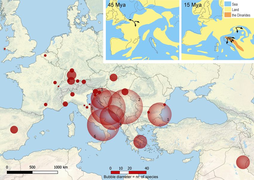
Fig. 1 Morphological and ecological diversity of Niphargus species. Adaptive radiation of Niphargus produced several morphotypes that inhabit distinct
subterranean habitats and niches. Different-sized morphotypes can occur together in cave lakes, and differently shaped morphotypes can occur together in
interstitial habitats17. These morphotypes evolved in at least five adaptive radiation events from hypothetical small-bodied ancestors from the shallow
interstitial habitat20,23. Appendages are abbreviated as app. Photographs used with author’s permission: Denis Copilaş-Ciocianu (shallow subterranean),
Teo Delić (all others).
disparity patterns in conjunction with clade age. For each divergent disparity of a clade against the disparity expected under the null
event (i.e. each node) we calculated the average of the disparities of model, showed insignificantly higher disparity than expected by the
all subclades whose ancestral lineages were present at that time, null model (MDI = 0.028, p = 0.4). We attribute this insignificant
standardised against the overall disparity. Disparity values near 0 result to the overall DTT dynamics where low disparities in early
imply that subclades contain relatively little variation present history cancelled out higher values during the last 15 Mya. The
within the entire clade, and most variation is partitioned as rank envelope test that tests how extreme the reconstructed DTT
differences between subclades. Values near 1 imply that subclades curve is compared to the simulated curves, showed that the DTT
contain a substantial proportion of the total variation, indicating curve falls outside the expected 95% confidence intervals of the null
that species within subclades have independently evolved to occupy model simulations (p-interval 0.0009–0.0270). Visual inspection of
similar regions of the ecomorphological space30,31. The observed the DTT plot (Fig. 2) showed that this deviation happened from 15
DTT curve was compared to the null hypothesis of neutral Mya onward. We also tested whether the evolutionary rates of the
evolution of morphology in which we simulated the relative eleven studied traits changed in time using the univariate node
disparities obtained from Brownian motion model30. The DTT height test31,32. The results were significant for all eleven traits,
plot suggested an early burst of disparity when the two major showing that the rate of their evolution indeed systematically
lineages arose ~35 million years ago, followed by 15 million years increased during the evolutionary history of the genus (Supple-
of continuous disparity decline that is in accord with neutral mentary Table 1 and Supplementary Fig. 3). Further exploration of
models of evolution. This decline is sharply ended by a significant multivariate evolutionary models applied to morphological traits33
recovery of morphological disparity at 15 Mya, pointing towards suggested that morphological diversification of the genus can be
independent diversification of ecological traits within subclades. best explained by a switch from the neutral Brownian motion
This phase of phenotypic diversification coincides with the increase model of morphological diversification to an early burst model at
in the rates of species accumulation and their ecological the time of presumed increase in diversification (15.5 Mya). This
diversification (Fig. 2: LTT and CTT). The morphological disparity shift suggests increased morphological diversification that finally
index (MDI)31 that measures the overall difference in the relative slowed down again at 2 Mya, possibly reflecting the emergence of
NATURE COMMUNICATIONS | (2021)12:3688 | https://doi.org/10.1038/s41467-021-24023-w | www.nature.com/naturecommunications 3ARTICLE NATURE COMMUNICATIONS | https://doi.org/10.1038/s41467-021-24023-w
a b c
(extremely elongated app.)
Phylogenetic clade labels (see b)
North Dinaric
6
A: Apeninne
ND: North Dinaric
Pa: Pannonian
Large stout, Daddy longleg
ln(lineages)
4
Po: Pontic
SD: South Dinaric
WB: West Balkan
2
Po,SD,WB
LTT
0.08 0.1 0
SD,WB
short app. stout, long app. long app.
nr. changes/∑ branch length
0.06
Big slender, Intermediate
SD,WB
0.04
CTT
West Balkan
A,ND
2.0
DTT
Disparity
1.0
ND,Pa,
Small stout,
Po,SD,WB
long app.
South Dinaric
0.0
40 30 20 10 0
Time [Mya]
Null model, mean (CTT, DTT) or median (LTT) value
Undistinct
95% distribution of the null model ND,Po,
Actual data, mean SD,WB
95 % confidence interval of 100 trees
Apeninne
Small pore slender,
A,Pa,
Po,WB
short app.
Unsaturated fissure system
Interstitial groundwater
Cave lake
stout, short app.
Cave stream
Shallow subterranean
Small pore
Specific chemistry Pa,
Po,WB
Pannonian
Small slender, short
appendages (app.)
A,ND,Po,
SD,WB
Pontic
Paleocene Eocene Oligocene Miocene Pliocene Pleistoc.
40 30 20 10 0
60 50 40 30 20 10 0
Ward's clustering height
Time [Mya]
ecological opportunity associated with the formation of karstic when novel habitat emerged at a grand scale27,34,35 (Fig. 3).
massifs, and the subsequent filling of the new ecological niches as These results are consistent with predictions from the
adaptive radiation progressed (Table 2). ecological theory of adaptive radiation, whereby the emer-
In summary, all diversification analyses suggested sudden gence of a large volume of novel and diverse habitat triggers
increases in the rates of species accumulation, morphological the evolutionary diversification of a lineage suited to this
evolution and ecological disparification at ~15 Mya—the time habitat.
4 NATURE COMMUNICATIONS | (2021)12:3688 | https://doi.org/10.1038/s41467-021-24023-w | www.nature.com/naturecommunicationsNATURE COMMUNICATIONS | https://doi.org/10.1038/s41467-021-24023-w ARTICLE Fig. 2 Three different aspects of the adaptive radiation of Niphargus. a Lineage diversification, ecological and morphological disparification notably accelerated ~15 Mya. The pattern is well visible on LTT, CTT and DTT plots. The time of an evolutionary shift is indicated by red arrows and grey line. b Calibrated phylogeny, species’ habitats and ancestral habitat reconstructions of Niphargus. Tips are labelled according to extant habitat. Pies on selected nodes represent reconstructed ancestral habitat (for complete reconstructions see Supplementary Fig. 2). Clades that were subjected to further analyses are coloured and named. c Cluster dendrogram based on eleven functional morphological traits. The same groups were partially recovered by PCA (Supplementary Fig. 8). The phylogenetic composition of morphological groups is labelled on the dendrogram. Cluster analysis shows that unrelated species evolved similar morphology (see clade’s acronyms on basal nodes of dendrogram). High morphological disparity presumably allowed high levels of syntopy and the formation of species-rich communities of closely related species. As an example, black and grey arrows on b and c point to species from a cave (Vjetrenica Cave System, Bosnia and Hercegovina) and interstitial (Sava river close to Medvode, Slovenia) communities, respectively. Note that many community members are closely related (same clade) but belong to different morphological clusters. Fig. 3 Geographical extent of the adaptive radiation of Niphargus. Bubbles represent the geographic position of subclades; their size reflects species numbers. Clades are numbered as follows: 1. Pontic, 2. Pannonian, 3. North Dinaric, 4. South Dinaric, 5. West Balkan and 6. Apennine clade. Inset: Phylogeny-based reconstruction of ancestral areas and directions of colonisation at 45 and 15 Mya, plotted on corresponding paleo maps, adapted after39,40. The geographic origin of species-rich subclades that arose through adaptive radiation corresponds to emerging karstic regions in South-Eastern Europe at about 15 Mya. The contemporary map was produced using QGIS77 and Esri World Physical Map78. Multiple independent radiations. The genus Niphargus com- Dinaric and the Apennine clade are younger, they started to prises several large, geographically well-defined clades. In diversify at 15–11 Mya (Supplementary Fig. 1). exceptional settings, large adaptive radiations can be the sum of The analyses of diversification (LTT plots and γ-test) suggested several independent radiations occurring in closely related that all clades display the pattern of an early burst of species lineages3,36. We selected six well-supported reciprocally mono- accumulation with onset between 15 and 5 Mya. CTT plots did phyletic clades that were geographically well-defined and suffi- not deviate from null models, but DTT analyses imply adaptive ciently large (N ≥ 25 species) to be explored for patterns of radiation patterns in the Pontic, Pannonian, West Balkan and the adaptive radiation by repeating LTT, CTT and DTT analyses on North Dinaric radiations (Table 4 and Fig. 4). Dynamics of each clade separately. They are distributed mostly in the karstic species accumulation and ecological disparification among these regions of Italy and South-Eastern Europe and spatially overlap to four clades differ (Table 4 and Fig. 4), possibly reflecting a various extent (Table 3, Fig. 2 and Supplementary Fig. 4). The differences in habitat diversity among regions where these Pontic and the Pannonian clade diverged from the rest of radiations unfolded or differences in the time of arrival of these Niphargus early (38 Mya, HPD 40–35 Mya), and split 29 Mya lineages in the novel habitats. The Apennine clade is composed (HPD 34–24 Mya). The South Dinaric, West Balkan, North mainly of morphologically similar, still undescribed species. NATURE COMMUNICATIONS | (2021)12:3688 | https://doi.org/10.1038/s41467-021-24023-w | www.nature.com/naturecommunications 5
ARTICLE                                                                                         NATURE COMMUNICATIONS | https://doi.org/10.1038/s41467-021-24023-w

 Table 1 Comparison of evolutionary models tested in order to identify the diversification pattern and rate shifts in the phylogeny
 of Niphargus.

 Model                                                             la1           mu1          K1                la2          mu2           K2               t-shift         AIC               AICw
 Shift in speciation rate                                          0.09          0            505.10            0.26         mu_1          K_1              15.70           2214.64           0.57
 Shift in speciation rate and carrying capacity                    0.12          0             45.15            0.25         mu_1          523.01           15.52           2217.02           0.17
 Shift in speciation rate, extinction rate and                     0.14          0.01          35.20            0.26         0             501.18           15.70           2217.21           0.16
 carrying capacity
 Shift in extinction rate and carrying capacity                    0.24          0.07          25.08            la_1         0             552.42           15.49           2217.97           0.11
 Shift in carrying capacity                                        0.20          0              1.56            la_1         mu_1          666.39           37.51           2238.11           0
 Diversity dependent model without shift                           0.21          0            609.67            /            /             /                /               2241.14           0

 Optimised parameters: la = speciation, mu = extinction, K = carrying capacity, t-shift = time of shift in Mya. The number denotes parameters before (1) or after (2) the shift. All optimising functions
 reached convergence.

Because of the lack of morphological data, we could not derive                                         subterranean adaptive radiations. We tested this hypothesis by
conclusions about the nature of this radiation.                                                        reconstructing ancestral habitats and ancestral areas of the six
   Finally, we explored whether these clade-level radiations show                                      Niphargus clades at 20 and 15 Mya. The evolution of ancestral
signs of between- or within clade convergent evolution. We used                                        ranges reconstructed under the Brownian motion model within a
SURFACE, a method that tests whether lineages have converged                                           Bayesian framework suggested that Niphargus originated in what
in phenotype without using a priori designations of ecomorphs37.                                       is now a part of Western Europe (Fig. 3). According to ancestral
It applies Hansen’s model of adaptive peaks38 modelled onto the                                        habitat reconstruction these species lived in and dispersed via
phylogeny and assumes that in the case of convergence similar                                          interstitial and shallow subterranean water systems to South-
phenotypes in different clades could be attributed to the same                                         Eastern Europe. The ancestral ranges of the six clades coincide
adaptive peaks. Three models that best explained the evolution of                                      with emerging carbonate islands of the Tethys Ocean and later
ecomorphological traits predicted 14–16 different adaptive peaks,                                      Paratethys Sea, nowadays representing the South-Eastern Alps,
of which 11–12 were found to be convergent whereas only three                                          the Dinaric Karst, and parts of the Carpathian arch (Fig. 3 and
to four were unique. These peaks partially correspond to clusters                                      Supplementary Data 2).
from the morphological analysis (Fig. 2). Of 11 convergent peaks,                                         These results suggest that Miocene karstification on island-like
two evolved multiple times within one clade, whereas nine peaks                                        parts of the continent apparently provided an ecological
evolved in two or more focal or non-focal clades. The results of                                       opportunity for groundwater-dwelling Niphargus that was able
the best model are illustrated in Supplementary Fig. 5.                                                to colonise and subsequently exploit the subterranean realm. The
   We tentatively conclude that at least four out of six large and                                     newly colonised empty space possibly triggered ecological
phylogenetically distinct clades could be considered as adaptive                                       divergence from the ancestral interstitial and shallow subterra-
radiations. Although showing some degree of convergence, the                                           nean forms, followed by morphological diversification and
radiations overall adapted to distinct sets of adaptive optima,                                        speciation within each independent radiation (Table 3).
especially so among the South-Eastern Europe clades.

                                                                                                       Discussion
Geographic origin of adaptive radiations. The increase in                                              The recovered patterns are concordant with predictions of
diversification and disparification around 15 Mya corresponds                                            adaptive radiation theory: a lineage with heritable ecological
to the emergence of karstic regions in South-Eastern Europe in                                         versatility to diversify that finds its ecological opportunity, will
the area of the modern South-Eastern Alps, the Dinarides and the                                       rapidly proliferate into ecologically different species, until the
Carpathians39,40. This area underwent a complex geological his-                                        available niches fill up5. We applied different methods which
tory. The collision of the European and Adriatic slabs during the                                      conservatively pinpointed that tree-wide shifts in evolutionary
Eocene (66–34 Mya) caused vivid tectonic movements that                                                dynamics spatially and temporally correspond to the onset of
resulted in drastic topographic changes41. In the Oligocene                                            ecological opportunity.
(32–23 Mya), the South-Eastern Alps and the Dinarides emerged                                             Niphargus originated from marine ancestors20 56–39 Mya,
from the surrounding seas, and the uplift of the Carpathians                                           in Western Europe as an interstitial amphipod. For the first
begun. The exposure of carbonate rocks of the Alpine-                                                  20–30 million years, speciation and ecological diversification
Carpathian-Dinaridic orogenic system to atmospheric processes                                          followed or even lagged behind neutral expectations. The genus
triggered karstification, i.e. the formation of caves and a variety of                                  presumably dispersed via coastal or brackish interstitial aquatic
other subterranean habitats17,27. This process began in the Oli-                                       habitats (Fig. 2) and accumulated genetic variation, which sup-
gocene and peaked in the Early Miocene (23–16 Mya). In that                                            ported rapid speciation that followed2.
period, mountain uplift continued and the three mountain ranges                                           Uplift of several carbonate platforms in South-Eastern Europe
acted as islands in the Paratethys Sea, occasionally connected                                         as islands in the Parathetys and subsequent karstification in the
during marine regressions. During the later Miocene (16–14                                             Early Miocene, 23–16 Mya, created new, ecologically diverse
Mya), a mosaic of saline and freshwater aquatic environments                                           subterranean habitats. Niphargus lineages colonised these new
and new emerging carbonate islands replaced the Paratethys,                                            predators- and competitor-free habitats and underwent several
which completely regressed from Late Miocene onwards (11                                               evolutionary radiations. At least five of these radiations exhibit
Mya)34,35.                                                                                             patterns of lineage diversification and trait evolution consistent
   The dynamic orogenesis of South-Eastern Europe opened a                                             with adaptive radiation, and the available information from
new unpopulated ecological space. These vast new freshwater                                            the undersampled clades in Greece and Iran42 hint there may
environments, initially free of predators and competitors,                                             be more such clades. Early habitat diversification, detected
constituted an ecological opportunity for lineages preadapted to                                       in tree-wide CTT analysis but not at the level of an individual
freshwater subterranean lifestyles to colonise and undergo                                             clade, may have constrained further clade-level morphological

6                       NATURE COMMUNICATIONS | (2021)12:3688 | https://doi.org/10.1038/s41467-021-24023-w | www.nature.com/naturecommunications
NATURE COMMUNICATIONS | https://doi.org/10.1038/s41467-021-24023-w ARTICLE
LTT DTT CTT
Morphology
Habitat
mean nr. of changes/total edge length
2.0
0.2
0
3
ln(lineages)
Pontic
disparity
2
1.0
0.1
0
1
0.0
0.0
0
0
2.0
0.2
Pannonian
3
0
2
1.0
0.1
0
1
0.0
0.0
0
0
South Dinaric
2.0
0.2
0
3
2
0.1
1.0
0
1
0.0
0.0
0
0
2.0
0.2
West Balkan
0
3
2
1.0
0.1
0
1
0.0
0.0
0
0
0.2
0
Apennine
3
2
0.1
0
1
0.0
0
0
2.0
North Dinaric
0.2
0
3
2
1.0
0.1
0
1
0.0
0.0
0
0
20 15 10 5 0 20 15 10 5 0 20 15 10 5 0
time [Mya] time [Mya] time [Mya]
Habitat Morphology
Unsaturated fissure system Large stout, long appendages Simulations, mean (CTT, DTT) or median (LTT) value
Interstitial groundwater Intermediate stout, long appendages Actual data, mean
Cave lake Small stout, long appendages 95% distribution of the null model
Cave stream Daddy longleg (extremely elongated appendages)
Shallow subterranean Big slender, short appendages
Specific chemistry Small slender, short appendages
Undistinct
Small pore stout, short appendages
Small pore slender, short appendages
Fig. 4 Evolution of six major Niphargus subclades. Zoomed phylogenies with plotted habitats and morphotypes (missing data not available), lineage
through time (LTT), changes through time (CTT) and disparity through time (DTT) plots. The DTT analysis could not be performed for the Apennine clade
due to too much missing data.
diversification. Subsequent morphological diversification of clades and allowed for uniquely species-rich communities, counting up
predominantly unfolded within one or few habitat types, like cave to nine species per site17,23 (Fig. 3). High local diversity combined
lakes (West Balkan and South Dinaric clade) or interstitial with multiple independent radiations can explain the extra-
groundwater (Pontic and Pannonian clade). This within- and ordinarily high number of species in the Dinaric Karst, a global
between-habitat diversification prompted high levels of sympatry subterranean biodiversity hotspot16. The mega adaptive radiation
NATURE COMMUNICATIONS | (2021)12:3688 | https://doi.org/10.1038/s41467-021-24023-w | www.nature.com/naturecommunications 7ARTICLE NATURE COMMUNICATIONS | https://doi.org/10.1038/s41467-021-24023-w
Table 2 Comparison of multivariate evolutionary models with or without shift, tested to identify the morphological
diversification pattern of the radiation of Niphargus.
Model logLik params AIC diff AICw
Brownian motion to early burst with independent drift −1420 9 2859 0 0.555
Ornstein–Uhlenbeck to early burst −1422 9 2862 2.78 0.138
Brownian motion to Ornstein–Uhlenbeck with independent drift −1420 11 2862 3.02 0.123
Brownian motion to early burst −1425 6 2862 3.36 0.104
Early burst to Ornstein–Uhlenbeck with independent drift −1420 12 2864 5.02 0.045
Ornstein–Uhlenbeck to early burst with independent drift −1420 12 2865 5.88 0.029
Ornstein–Uhlenbeck −1426 8 2868 9.4 0.005
Early burst to Ornstein–Uhlenbeck −1427 9 2871 12.31 0.001
Brownian motion to Ornstein–Uhlenbeck −1454 8 2925 65.8 0
Early burst to Brownian motion −1490 6 2991 132.6 0
Ornstein–Uhlenbeck to Brownian motion −1489 8 2994 134.8 0
Early burst to Brownian motion with independent drift −1489 9 2996 137.5 0
Ornstein–Uhlenbeck to Brownian motion with independent drift −1890.18 21 3822.36 250.55 0
Brownian motion −1915.91 9 3849.82 278.02 0
Early burst −1915.91 10 3851.82 280.02 0
Table 3 Summary of diversification patterns of the genus Niphargus and its major subclades.
Clade Nr. of species Distribution Nr. of habitats Nr. of Diversification
analysed occupied morphotypes pattern
Niphargus genus 377 From Ireland to Iran 6 9 Adaptive radiation
Pontic 28 Eastern Europe to Crimean Peninsula 6 6 Adaptive radiation
Pannonian 41 Northern Italy, Pannonian Basin and Carpathian arch 4 3 Adaptive radiation
South Dinaric 29 Southern Dinaric Region, Adriatic Islands, southern parts 5 6 Adaptive radiation
of Apennine Peninsula
West Balkan 41 North-Western Balkan 6 8 Adaptive radiation
Apennine 38 Apennine Peninsula, Eastern coasts of Adriatic Sea 5 3 Non-adaptive
radiation
North Dinaric 25 Northern Dinaric Region, Adriatic Islands, central parts 4 4 Adaptive radiation
of Apennine Peninsula
Table 4 Lineage through time (LTT), changes through time (CTT) and disparity through time (DTT) statistics for six major
Niphargus subclades.
Clade LTT statistics DTT statistics (MDI; p-interval of ranked envelope test) CTT
Pontic γ = −3.9, p-value = 0 0.15; 0.001–0.025 Random
Pannonian γ = −2.6, p-value = 0.009 0.17; 0.001–0.026 Random
South Dinaric γ = −1.8, p-value = 0.076 0.06; 0.364–0.371 Random
West Balkan γ = −3.1, p-value = 0.002 0.14, 0.001–0.033 Random
Apennine γ = −3.9, p-value = 0 n.a.a Recent increase
North Dinaric γ = −2.9, p-value = 0.004 0.15; 0.001–0.028 Random
aThe DTT analysis could not be accurately performed for the Apennine clade due to missing data.
of the amphipod genus Niphargus that generated 20–25% of all clades in the tree of life and large biomes1,3, these studies support
freshwater amphipods in the World, can be seen as an exception Simpson’s idea that adaptive radiations are a universal phenom-
to the widespread pattern where the fauna of present-day Europe enon and an important global generator of biodiversity5.
contributes relatively little to global biological diversity8,43. We noted a pattern of independent regional adaptive radiations
At a first glance, it seems paradoxical that what might be the in several clades. This mechanism likely contributed to the out-
largest surviving pre-Pleistocene adaptive radiation on the Eur- standing species richness of Niphargus, across different geo-
opean continent took place in an environment as desolate as the graphic scales22. Consequently, the Niphargus radiation is similar
karstic underground. The environment is ecologically simple, in size to the radiations of amphipods from the Baikal lake44,47.
permanently dark, and nutrient-deprived27. As it lacks primary Evolution of distinct phenotypes in independent adaptive radia-
producers, ecological opportunity—an environmental prerequisite tions as already reported in plants and vertebrates1,3,48 may be
for adaptive radiation24—does seem unlikely to be fulfilled. more common than previously thought, yet overlooked in studies
However, adaptive radiations have been reported from other oli- that were narrow in taxonomic focus49.
gotrophic habitats, including the abyssal zone of deep lakes44, the In the Western Palearctic, ancient in situ adaptive radiations
deep sea45 and the Antarctic46. Along with studies from major that predate the climate chaos of the Pleistocene do not reveal
8 NATURE COMMUNICATIONS | (2021)12:3688 | https://doi.org/10.1038/s41467-021-24023-w | www.nature.com/naturecommunicationsNATURE COMMUNICATIONS | https://doi.org/10.1038/s41467-021-24023-w ARTICLE
themselves readily. The case of Niphargus suggests that one must Phylogeny and molecular clock. The sequences were aligned in Geneious with
search for them in environments that are insulated against the MAFFT v7.38860 plugin, using E-INS-i algorithm with scoring matrix 1PAM/k = 2
with the highest gap penalty. Alignments were concatenated in Geneious. We used
effects of climate fluctuations. Climate history clearly had a strong Gblocks61 to remove gap-rich regions from the alignments of non-coding markers
impact on the rise and loss of biodiversity in Europe4. Climatic prior to phylogenetic analysis, with settings for less stringent selection.
perturbations wiped out faunas that had evolved in ancient We used Partition Finder 2 for determining the optimal substitution model for
adaptive radiations4. Notably, these Pleistocene extinctions cre- each partition62,63 under the corrected Akaike information criterion (AICc). The
ated ecological opportunity24 for multiple Holocene adaptive selected optimal substitution models are listed in Supplementary Table 5.
Backbone phylogenies (301 Niphargus MOTUs with at least two fragments and
radiations of limited extent11,12. Only in ecosystems that were five outgroups MOTUs) were reconstructed using Bayesian inference (BI) and
shaded from the devastating effects of climatic fluctuations could maximum-likelihood (ML) in MrBayes 3.2.664 and IQ-TREE 1.6.665, respectively
the full historical richness of older radiations be preserved. If this (Supplementary Fig. 6 and 7). In MrBayes we run two simultaneous independent
hypothesis is correct, further relic adaptive radiations should be runs with eight chains each for 200 million generations, sampled every 20,000th
generation. We discarded the first 25% of trees as burn-in and calculated the 50%
expected among taxa from environments that were so far majority-rule consensus tree. Convergence was assessed through average standard
neglected, such as the subterranean realm and deep soil21,50. deviation of split frequencies, LnL trace plots, potential scale reduction factor
Whether or not we shall be able to discover them depends also on (PSRF), and the effective sample size. Results were analysed in Tracer 1.766. The
the progression of adverse anthropogenic impacts: while resilient ML tree was calculated in IQ-TREE using the same evolutionary models as in BI,
with ultrafast bootstrap approximation (UFBoot)67, H-like approximate likelihood
and buffered from ecological fluctuations throughout geological ratio test62 and -bnni function to reduce the risk of overestimating branch supports
history, these species are not immune to habitat destruction and with UFBoot. Phylogenetic analyses were run on the CIPRES Science Gateway
may be particularly vulnerable to pollution51. (http://www.phylo.org). For the molecular clock analysis, we built a time-calibrated
chronogram of all 377 Niphargus MOTUs with BEAST 268 (Supplementary Fig. 1).
We set four internal calibration points. (1) Fossil: ‘modern-looking’ Niphargus
Methods fossils from Eocene Baltic amber estimated to be 40–50 million years old69. Their
Dataset. The molecular dataset consisted of all available genetic data for described morphology resembles modern Niphargus species with distinct pectinate dactyls.
and undescribed Niphargus sensu lato species. Several species formally included in We placed the calibration point on the node where this particular morphological
different niphargid genera (Carinurella, Haploginglymus, Chaetoniphargus, character occurs for the first time (N. ladmiraulti). (2) European niphargids: the
Niphargobates) are nested within the Niphargus radiation. Some of them are final submergence of the land bridges between Eurasia and North America
monophyletic, and others are not. Although the monophyly of Niphargus sensu presumably prevented the dispersal of niphargids towards Greenland and North
lato was established multiple times25,29,52 the nested genera were never formally America. If so, niphargids are most probably younger than the three natural
synonymized, and thus we use the valid nomenclature. Sequences included newly bridges connecting North Europe, Greenland and North America, which existed
acquired and previously unpublished sequences (SubBio Database53, accessed on between 57 and 71 Mya70. (3) Crete clade: species from Crete form a highly
20. 2. 2018) and existing GenBank records54. To account for cryptic species, we supported monophyletic group with closest relatives on mainland Greece. The
substituted nominal species with MOTUs, molecularly delimited in the previous calibration point relies on the isolation of Crete Island from the mainland that
works25,29,55,56. Most of these species were delimited using multilocus species happened at the end of the Messinian salinity crisis (5.3–5 Mya)71. (4) Middle East
delimitations; only a smaller fraction was delimited using only mitochondrial COI clade: species from Lebanon to Iran form a highly supported monophyletic group
gene sequences. In these cases, we relied on delimitations using the most con- of eastern Niphargus. With rising sea levels and the opening of the connection
servative delimitation approach, i.e. a 16% patristic distance treshold20. In total, our between Paratethys and the Mediterranean basin 11–7 Mya, the Dinarides and
dataset counted 377 MOTUs of Niphargus, rooted with five outgroup species from eastern mainland became separated39,40. Technical details of calibration points are
the genera Niphargellus, Microniphargus and Pseudoniphargus57. Of these, 223 given in Supplementary Table 6.
MOTUs corresponded to nominal species (50% of the 447 nominal Niphargus To assess the degree of incongruence among the calibration points, we run
species (WORMS58)); 154 MOTUs are not yet formally named. analyses using each calibration point separately and compared age distributions for
Ecological information on the studied species was extracted from literature main nodes (Supplementary Table 2). For each gene partition we used a set of
compiled in the European Groundwater Crustacean Database (EGCD)16, from own priors as followed: linked birth-death tree model, unlinked site models as in
data and from databased field notes (SubBio Database53, accessed on 20. 2. 2018). previous analyses, with fixed mean substitution rate and relaxed clock log-normal
We assigned 331 species to six habitat categories ((1) unsaturated fissure system, distribution with estimated clock rate. We used default settings of distributions of
(2) interstitial, (3) cave lakes, (4) cave streams, (5) shallow subterranean and all estimates. We run the analyses for 200 million generations, sampled every
(6) groundwater with specific chemistry (brackish, sulfidic, acidic or mineral)). 20,000 generations. The first 25% of trees were discarded as burn-in.
Species for which ecological data are lacking and MOTUs identified from published All subsequent analyses were run on the clock-calibrated trees of Niphargus
GenBank sequences were left uncharacterised. Morphometric traits included 11 (377 MOTUs). To account for phylogenetic uncertainty, we used a random subset
morphological continuous traits known to correspond to habitat properties17,23. of 100 calibrated trees and maximum clade credibility (MCC) tree. To assess the
The traits were measured using standard protocol59. Briefly, we partially dissected potential influence of missing sequence data in the dataset, we repeated the BEAST
the specimens, mounted them on glycerol slides, and photographed them using a 2 and through time analyses (LTT, CTT, DTT and subsequent statistics) on the
ColorView III camera mounted on an Olympus SZX stereomicroscope. We subset of 301 Niphargus MOTUs with at least two markers (Supplementary Fig. 8).
measured the photographs using the programme CellB (Olympus, 2008) to the The results were congruent with the results obtained from the extended dataset and
precision of 0.01 mm. Depending on the availability of material, we measured showed a negligible effect of missing data on the final phylogeny reconstruction
between 1 and 20 individuals per species. In many species, samples were heavily and downstream analyses.
damaged. In such cases, we supplemented the measurements with information
available in species descriptions. For 26 species we had no appropriate samples, but
we could extract measurements from the original descriptions. In total, we General strategy in diversification analyses. The theory of adaptive radiation
compiled a morphometric dataset for 256 species. Ethical issues are not applicable predicts an initial burst of speciation and disparification rates followed by a decline
to this study. as the available niches fill. We tested this prediction using two alternative strategies.
First, we analysed species diversification and ecological as well as morphological
disparification through time against simulated null models. Secondly, we tested
DNA sequences. Genomic DNA was extracted using the GenElute Mammalian which evolutionary models of diversification and morphological disparification
Genomic DNA Miniprep Kit (Sigma-Aldrich, United States). We amplified eight best fit to our data.
phylogenetically informative markers: the mitochondrial cytochrome oxidase I The analyses were run on the whole dataset and repeated on six selected clades
(COI) gene, two segments of the 28S rRNA gene, the histone H3 gene (H3), a part that satisfied three conditions: high node support, a high number (>25) of species
of the 18S rRNA gene, as well as partial sequences of the phosphoenolpyruvate and geographically well-defined distribution within limited areas (Pontic,
carboxykinase (PEPCK), glutamyl-prolyl-tRNA synthetase gene (EPRS), heat shock Pannonian, North Dinaric, South Dinaric, West Balkan and Apennine clade).
protein 70 (HSP70) and arginine kinase (ArgKin) genes. Oligonucleotide primers MOTUs with missing morphometric data were excluded from the DTT and
and amplification protocols are given in Supplementary Table 4. Markers that were multivariate modelling analyses. The clades are marked on the chronogram
sequenced from several specimens of the same MOTU are marked as chimaeras in (Fig. 2). All analyses were run in R v.3.6.072, using packages vegan v.2.5-5, phytools
Supplementary Data 1. To exclude misidentification, chimeric specimens were v.0.6-60, geiger v.2.0.6.1, DDD v.4.0, surface v.0.5, mvMorph v.1.1.0, readxl v.1.3.1,
from the same or nearby localities and with identical sequences of overlapping RColorBrewer v.1.1-2, ggplot2 v.3.3.3, grid v.4.0.3, gridExtra v.2.3, dplyr v.1.0.2 and
markers of high resolution (e.g. COI). In the dataset, 301 MOTUs were represented plyr v.1.8.6.
by at least two fragments. For 76 MOTUs only the COI fragment was available.
Nucleotide sequences were obtained by the Macrogen Europe laboratory
(Amsterdam, Netherlands) using amplification primers and bi-directional Sanger Estimation of speciation dynamics. The diversification dynamics was assessed
sequencing. We edited and assembled chromatograms in Geneious 11.0.3. from the lineage through time (LTT) plot on 100 randomly chosen trees26, together
(Biomatters Ltd, New Zealand). with the γ-test73. The γ-test asks whether per-lineage speciation and extinction
NATURE COMMUNICATIONS | (2021)12:3688 | https://doi.org/10.1038/s41467-021-24023-w | www.nature.com/naturecommunications 9ARTICLE NATURE COMMUNICATIONS | https://doi.org/10.1038/s41467-021-24023-w
rates have remained constant through time. A deviation from 0 indicates a change explicitly modelled in Hansen’s model of trait evolution using two parameters, trait
in speciation rates. As a null model, we simulated 1000 trees under the pure birth value and strength of stabilising selection38. The assessment of convergence is
assumption, since the analyses under the birth-death assumption did not differ and made in two steps. In the first step, SURFACE successively fits a series of adaptive
the estimated extinction rates were negligible. peaks onto a phylogeny using stepwise AIC. In turn, it simplifies the model by
A change in diversification rate may be related to differences in rates of merging similar adaptive peaks using stepwise AIC. These adaptive peaks may
extinction or speciation. We searched for the best model that describes the course point to convergent evolution37. The adaptive peaks were inferred using the first
of diversification. To do this, we first fitted different models that account for shifts two axes of phylogenetically corrected PCA (explaining 97.5% of total variance) as
in diversification parameters: speciation rate (λ), extinction rate (μ) and clade- a surrogate for morphological data, and the MCC phylogeny. We ran two analyses.
carrying capacity (K)74. Specifically, we tested whether our data is best described by First, we used the entire genus phylogeny. This analysis was not sensitive enough to
a simple birth-death model with constant λ and μ, diversity dependent models with capture evolutionary dynamics in the Pannonian and Pontic clade. These species
incorporated K, or models with a shift in time: shift in one or more parameters λ, K are generally small-pore inhabitants and on average an order of magnitude smaller
and μ. We also estimated the time of the shift. The fit of the models was compared than in other clades. Relative morphological variation within these two clades is
using Akaike weights. smaller as compared to variation among larger species and traits that vary in these
clades explain only the fourth PCA axis, which was not used in the analysis. The
genus-level analysis identified one and two adaptive peaks for Pontic and Pan-
Analysis of ecological diversification. The ecological diversification of Niphargus nonian clade, respectively. To account for a potential lack of sensitivity, we repe-
species was estimated using changes through time plots (CTT)26. First, discrete ated the analysis on a pruned tree, composed of only two clades. Indeed, this
habitat traits were mapped onto a phylogenetic MCC tree using stochastic char- analysis identified additional adaptive peaks (not reported in the main text). The
acter mapping, assessed from 1000 simulated stochastic character histories using results of both analyses are presented in Supplementary Fig. 5.
the tip states on the tree and a continuous-time reversible Markov model of trait
evolution, fitted on the phylogeny75. The evolutionary rates of transition between
different ecologies (i.e. transition matrix Q) were estimated from the data. We Ancestral habitat and ancestral area reconstruction. Ancestral habitat was
plotted the mean number of character changes per sum of branch lengths in a given estimated from the species habitats that were mapped onto a phylogenetic MCC
time period from a set of stochastic map trees against evolutionary time. The tree using stochastic character mapping. We ran 1000 simulated stochastic char-
empirical CTT was tested against the assumption of constant evolution inferred acter histories using the tip states on the tree and a continuous-time reversible
from a null model. The null Brownian-motion model was generated from Markov model of trait evolution, fitted on the phylogeny75. The evolutionary rates
1000 simulated stochastic character maps using the tree and the observed transition of transition between different habitats (i.e. transition matrix Q) were estimated
matrix Q26. from the data. Species with unknown habitat were given equal probability for each
state. We reconstructed ancestral geographical areas for six analysed clades using
the longitude and latitude of our samples mapped onto phylogeny. The evolution
Analysis of morphological diversification. Morphological diversification was of ancestral ranges was mapped on the MCC tree under the Brownian motion
examined using disparity through time plots (DTT), the morphological disparity model within a Bayesian framework implemented in Geo Model in BayesTraits
index (MDI), the ranked confidence envelope test, the node height test, and by V3.0.176. The Geo model maps longitude and latitude onto a three-dimensional
searching for the best-fitting model of trait evolution. We used eleven continuous Cartesian coordinates system, and thus eliminates error in reconstructions due to
morphological traits (see Dataset). Morphological traits were treated as follows. the spherical nature of the Earth. We ran 11 million MCMC generations, sampled
First, for each trait, we calculated mean values per species. In subsequent analyses, every 10,000th, discarded the first million as a burn-in, and checked the trace for
body length was used as a raw variable, whereas other traits were corrected for the convergence. The 95% confidence intervals for regions of origin were determined
body length. We regressed all traits onto body length and calculated phylogen- such that we discarded 5% of the reconstructed sites that were farthest away from
etically corrected residuals using phylogenetic generalised least squares26. DTT the centroid. The remaining estimated points of origin were plotted onto paleo
plots were calculated to examine the course of morphological diversification30. The maps, adapted from the available literature39,40. Maps were produced using
disparity value at each node represents a variance-related estimate of the dispersion QGIS77, and Esri World Physical Map78.
of points in multivariate space insensitive to sample size, measured as average
squared Euclidean distance among all pairs of species of given subclade30. Disparity Reporting summary. Further information on research design is available in the Nature
values of subclades were divided by the overall disparity of the clade. For each Research Reporting Summary linked to this article.
divergent event, the average of the relative disparities of all subclades whose
ancestral lineages were present at that time was calculated and the empirical DTT
curve was compared to null model expectations, generated from 1000 simulated Data availability
trait distributions obtained from a model of evolution by Brownian motion. We Sequence data have been deposited in GenBank. Vouchers, GenBank accession numbers
tested the significance of deviation from expected disparity by two methods, with hyperlinks to GenBank, spatial coordinates, morphometric data, and ecological data
pairwise and ranked confidence envelope tests (only results for more stringent, of samples are listed in Supplementary Data 1, 3 and 4. Newly obtained sequences are
ranked confidence envelope are shown). Second, we calculated the morphological available in GenBank under accession numbers MT191378–MT192029, MZ270543 and
disparity index (MDI) that measures the overall difference in the relative disparity MZ295224. Alignments and settings for phylogenetic analyses are available on Zenodo
of a clade compared with that expected under the null model31. (https://doi.org/10.5281/zenodo.4779097)79. European Groundwater Crustacean
We also performed the univariate node height test that searches for a significant Database (EGCD) used for compiling ecological information of species is accessible
correlation between phylogenetically independent contrasts and the heights of the on http://www.freshwatermetadata.eu/metadb/bf_mdb_view.php?entryID=BF73.
nodes at which they are generated32. The height of a node is defined as the absolute
distance between the root and the most recent common ancestor of the pair from
which the contrast is generated. Significant correlation indicates that the rate of Code availability
trait evolution is changing systematically through the tree32. We performed a node All code used in analyses is available on Zenodo (https://doi.org/10.5281/
height test for each of the 11 traits separately. zenodo.4779097).
Finally, we explored which evolutionary model best describes trait evolution
within a multi-trait framework that accounts for trait covariances33. To reduce the
number of parameters, we calculated phylogenetically corrected PCA, and used the Received: 11 September 2020; Accepted: 1 June 2021;
first two axes (cumulative variance 97.5%, Supplementary Table 3). We fitted
different multivariate models of continuous trait evolution to our tree: Brownian
Motion (BM), Early Burst (EB), ACcelerate-DeCelerate (ACDC),
Ornstein–Uhlenbeck and models with a shift in time from one regime to another.
As a shifting point, we took the estimated time of change of diversification rates
(see Species diversification). The fit of the models was estimated using Akaike References
weights33. 1. Alfaro, M. E. et al. Nine exceptional radiations plus high turnover explain
To illustrate morphological variability and parallel evolution of morphotypes we species diversity in jawed vertebrates. PNAS 106, 134–14 (2009).
used hierarchical clustering using Ward’s method, using the same dataset as for 2. Seehausen, O. Process and pattern in cichlid radiations - inferences for
DTT. We identified nine different clusters, well segregated also when plotted onto understanding unusually high rates of evolutionary diversification. N. Phytol.
the first two PCA axes (see above) (Supplementary Fig. 9). 207, 304–312 (2015).
3. Tank, D. C. et al. Nested radiations and the pulse of angiosperm
Analysis of convergence. To test for convergence on the macroevolutionary diversification: Increased diversification rates often follow whole genome
adaptive landscape we used SURFACE (acronym for ‘SURFACE Uses Regime duplications. N. Phytol. 207, 454–467 (2015).
Fitting with AIC to model Convergent Evolution’). SURFACE tests for lineages’ 4. Neubauer, T. A., Harzhauser, M., Georgopoulou, E., Kroh, A. & Mandic, O.
convergence in phenotype without using a priori designations of ecomorphs37. Tectonics, climate, and the rise and demise of continental aquatic species
Briefly, within adaptive radiation, different lineages may evolve into distinct eco- richness hotspots. PNAS 112, 11478–11483 (2015).
logical niches, each occupying its own adaptive peak. These adaptive peaks are 5. Schluter, D. The Ecology of Adaptive Radiation (Oxford University Press, 2000).
10 NATURE COMMUNICATIONS | (2021)12:3688 | https://doi.org/10.1038/s41467-021-24023-w | www.nature.com/naturecommunicationsNATURE COMMUNICATIONS | https://doi.org/10.1038/s41467-021-24023-w ARTICLE
6. Schenk, J. J., Rowe, K. C. & Steppan, S. J. Ecological opportunity and 38. Hansen, T. F. Stabilizing selection and the comparative analysis of adaptation.
incumbency in the diversification of repeated continental colonizations by Evolution 51, 1341 (1997).
muroid rodents. Syst. Biol. 62, 837–864 (2013). 39. Popov, S. V., Rögl, F. & Rozanov, A. Y. Lithological-Paleogeographic Maps of
7. Jenkins, N. C., Pimm, S. L. & Joppa, L. N. Global vertebrate diversity and Paratethys: 10 Maps Late Eocene to Pliocene (Schweizerbart’sche
conservation. PNAS 110, E2602–E2610 (2013). Verlagsbuchhandlung, 2004).
8. Kier, G. et al. A global assessment of endemism and species richness across 40. Barrier, E., Vrielynck, B., Brouillet, J. F. & Brunet, M. F. Paleotectonic
island and mainland regions. PNAS 106, 9322–9327 (2009). Reconstruction of the Central Tethyan Realm. Tectonono-Sedimentary-
9. Reyjol, Y. et al. Patterns in species richness and endemism of European Palinspastic Maps from Late Permian to Pliocene (CCGM/CGMW, 2018).
freshwater fish. Glob. Ecol. Biogeogr. 16, 65–75 (2007). 41. Handy, M. R., Ustaszewski, K. & Kissling, E. Reconstructing the
10. Hewitt, G. The genetic legacy of the Quaternary ice ages. Nature 405, 907–913 Alps–Carpathians–Dinarides as a key to understanding switches in
(2000). subduction polarity, slab gaps and surface motion. Int. J. Earth. Sci. 104, 1–26
11. Albrecht, C., Trajanovski, S., Kuhn, K., Streit, B. & Wilke, T. Rapid evolution (2015).
of an ancient lake species flock: freshwater limpets (Gastropoda: Ancylidae) in 42. Esmaeili-Rineh, S., Sari, A., Delić, T., Moškrič, A. & Fišer, C. Molecular
the Balkan lake Ohrid. Org. Divers. Evol. 6, 294–307 (2006). phylogeny of the subterranean genus Niphargus (Crustacea: Amphipoda) in
12. Vonlanthen, P. et al. Eutrophication causes speciation reversal in whitefish the Middle East: a comparison with European Niphargids. Zool. J. Linn. Soc.
adaptive radiations. Nature 482, 357–362 (2012). 175, 812–826 (2015).
13. Renema, W. et al. Hopping hotspots: Global shifts in marine biodiversity. 43. Pimm, S. L. et al. The biodiversity of species and their rates of extinction,
Science 321, 654–657 (2008). distribution, and protection. Science 344, 6187 (2014).
14. Gargani, J. & Rigollet, C. Mediterranean Sea level variations during the 44. Hou, Z. & Sket, B. A review of Gammaridae (Crustacea: Amphipoda): the
Messinian salinity crisis. Geophys. Res. Lett. 34, 1–5 (2007). family extent, its evolutionary history, and taxonomic redefinition of genera.
15. Culver, D. C. et al. The mid-latitude biodiversity ridge in terrestrial cave fauna. Zool. J. Linn. Soc. 176, 323–348 (2016).
Ecography 29, 120–128 (2006). 45. Corrigan, L. J., Horton, T., Fotherby, H., White, T. A. & Hoelzel, A. R.
16. Zagmajster, M. et al. Geographic variation in range size and beta diversity of Adaptive evolution of deep‐sea amphipods from the superfamily
groundwater crustaceans: Insights from habitats with low thermal seasonality. lysiassanoidea in the North Atlantic. Evol. Biol. 41, 154–165 (2014).
Glob. Ecol. Biogeogr. 23, 1135–1145 (2014). 46. Clarke, A. & Johnston, I. A. Evolution and adaptive radiation of Antarctic
17. Trontelj, P., Blejec, A. & Fišer, C. Ecomorphological convergence of cave fishes. Trends Ecol. Evol. 11, 212–218 (1996).
communities. Evolution 66, 3852–3865 (2012). 47. Macdonald, K. S. 3rd, Yampolsky, L. & Duffy, J. E. Molecular and
18. Trontelj, P., Borko, Š. & Delić, T. Testing the uniqueness of deep terrestrial morphological evolution of the amphipod radiation of Lake Baikal. Mol.
life. Sci. Rep. 9, 15188 (2019). Phylogenet. Evol. 35, 323–343 (2005).
19. Morvan, C. et al. Timetree of Aselloidea reveals species diversification 48. Elmer, K. R. et al. Parallel evolution of Nicaraguan crater lake cichlid fishes via
dynamics in groundwater. Syst. Biol. 62, 512–522 (2013). non-parallel routes. Nat. Commun. 5, 5168 (2014).
20. Eme, D. et al. Do cryptic species matter in macroecology? Sequencing 49. Esquerré, D. & Keogh, J. S. Parallel selective pressures drive convergent
European groundwater crustaceans yields smaller ranges but does not diversification of phenotypes in pythons and boas. Ecol. Lett. 19, 800–809
challenge biodiversity determinants. Ecography 41, 424–436 (2017). (2016).
21. Lukić, M., Delić, T., Pavlek, M., Deharveng, L. & Zagmajster, M. Distribution 50. von Saltzwedel, H., Scheu, S. & Schaefer, I. Founder events and pre-glacial
pattern and radiation of the European subterranean genus Verhoeffiella divergences shape the genetic structure of European Collembola species. BMC
(Collembola, Entomobryidae). Zool. Scr. 49, 86–100 (2019). Evol. Biol. 16, 148 (2016).
22. Väinölä, R. et al. Global diversity of amphipods (Amphipoda; Crustacea) in 51. Mammola, S. et al. Scientists’ warning on the conservation of subterranean
freshwater. Hydrobiologia 595, 241–255 (2008). ecosystems. BioScience 69, 641–650 (2019).
23. Fišer, C., Delić, T., Luštik, R., Zagmajster, M. & Altermatt, F. Niches within a 52. Lefébure, T., Douady, C. J., Malard, F. & Gibert, J. Testing dispersal and
niche: ecological differentiation of subterranean amphipods across Europe’s cryptic diversity in a widely distributed groundwater amphipod (Niphargus
interstitial waters. Ecography 42, 1212–1223 (2019). rhenorhodanensis). Mol. Phylogenet. Evol. 42, 676–686 (2007).
24. Stroud, J. T. & Losos, J. B. Ecological opportunity and adaptive radiation. 53. Zagmajster, M., Turjak, M., & Sket, B. Database on subterranean biodiversity
Annu. Rev. Ecol. Evol. Syst. 47, 507–532 (2016). of the Dinarides and neighboring regions – SubBioDatabase. In 21st
25. McInerney, C. E. et al. The ancient Britons: groundwater fauna survived International Conference on Subterranean Biology, 2–7 September, 2012,
extreme climate change over tens of millions of years across NW Europe. Mol. Košice, Slovakia, Abstract book (ed. Kováč, Ĺ., et al.) 116–117 https://doi.org/
Ecol. 23, 1153–1166 (2014). 10.13140/2.1.4518.0487 (Pavol Jozef Šafárik University, Košice, 2012).
26. Revell, L. J. phytools: An R package for phylogenetic comparative biology (and 54. Clark, K., Karsch-Mizrachi, I., Lipman, D. J., Ostell, J. & Sayers, E. W.
other things). Methods Ecol. Evol. 3, 217–223 (2012). GenBank. Nucleic Acids Res. 44, D67–D72 (2016).
27. Culver, D. C. & Pipan, T. The Biology of Caves and Other Subterranean 55. Fišer, C. et al. Translating Niphargus barcodes from Switzerland into
Habitats 2nd edn (OUP, 2019). taxonomy with a description of two new species (Amphipoda, Niphargidae).
28. Kralj-Fišer, S. et al. The interplay between habitat use, morphology and ZooKeys 760, 113–141 (2018).
locomotion in subterranean crustaceans of the genus. Niphargus. Zool. 139, 56. Jurado-Rivera, J. A. et al. Molecular systematics of Haploginglymus, a genus of
125742 (2020). subterranean amphipods endemic to the Iberian Peninsula (Amphipoda:
29. Delić, T., Trontelj, P., Rendoš, M. & Fišer, C. The importance of naming Niphargidae). Contrib. Zool. 86, 239–260 (2017).
cryptic species and the conservation of endemic subterranean amphipods. Sci. 57. Copilaş-Ciocianu, D., Borko, Š. & Fišer, C. The late blooming amphipods:
Rep. 7, 1–12 (2017). global change promoted post-Jurassic ecological radiation despite Palaeozoic
30. Harmon, L. J., Schulte, J. A., Losos, J. B. & Larson, A. Tempo and mode of origin. Mol. Phylogenet. Evol. 143, 106664 (2020).
evolutionary radiation in iguanian lizards. Science 301, 961–964 (2003). 58. Horton, T. et al. World Register of Marine Species. https://www.
31. Murrell, D. J. A global envelope test to detect non‐random bursts of trait marinespecies.org. Accessed 6 Mar 2020 (2020).
evolution. Methods Ecol. Evol. 9, 1739–1748 (2018). 59. Fišer, C., Trontelj, P., Luštrik, R. & Sket, B. Toward a unified taxonomy of
32. Freckleton, R. P. & Harvey, P. H. Detecting non-Brownian trait evolution in Niphargus (Crustacea: Amphipoda): a review of morphological variability.
adaptive radiations. PLoS Biol. 4, e373 (2006). Zootaxa 2061, 1–22 (2009).
33. Clavel, J., Escarguel, G. & Merceron, G. mvMORPH: an R package for fitting 60. Katoh, K. & Standley, D. M. MAFFT multiple sequence alignment software
multivariate evolutionary models to morphometric data. Methods Ecol. Evol. version 7: improvements in performance and usability. Mol. Biol. Evol. 30,
6, 1311–1319 (2015). 772–780 (2013).
34. Kováč, M. et al. The central paratethyspalaeoceanography: a water circulation 61. Talavera, G. & Castresana, J. Improvement of phylogenies after removing
model based on microfossilproxies, climate, and changes of depositional divergent and ambiguously aligned blocks from protein sequence alignments.
environment. Acta Geol. Slov. 9, 75–114 (2017). Syst. Biol. 56, 564–577 (2007).
35. Kováč, M. et al. Towards better correlation of the Central Paratethys regional 62. Guindon, S. et al. New algorithms and methods to estimate maximum-
time scale with the standard geological time scale of the Miocene Epoch. Geol. likelihood phylogenies: assessing the performance of PhyML 3.0. Syst. Biol. 59,
Carpath. 69, 283–300 (2018). 307–321 (2010).
36. Mahler, D. L., Ingram, T., Revell, L. J. & Losos, J. B. Exceptional convergence 63. Lanfear, R., Calcott, B., Ho, S. Y. & Guindon, S. PartitionFinder: combined
on the macroevolutionary landscape in island lizard radiations. Science 341, selection of partitioning schemes and substitution models for phylogenetic
6143 (2013). analyses. Mol. Biol. Evol. 29, 1695–1701 (2012).
37. Ingram, T. & Mahler, D. SURFACE: detecting convergent evolution from 64. Ronquist, F. et al. MrBayes 3.2: efficient Bayesian phylogenetic inference
comparative data by fitting Ornstein‐Uhlenbeck models with stepwise Akaike and model choice across a large model space. Syst. Biol. 61, 539–542
Information Criterion. Methods Ecol. Evol. 4, 416–425 (2013). (2012).
NATURE COMMUNICATIONS | (2021)12:3688 | https://doi.org/10.1038/s41467-021-24023-w | www.nature.com/naturecommunications 11You can also read