Tree mortality in western U.S. forests forecasted using forest inventory and Random Forest classification
←
→
Page content transcription
If your browser does not render page correctly, please read the page content below
MACROSYSTEMS ECOLOGY

        Tree mortality in western U.S. forests forecasted using forest
               inventory and Random Forest classification
         BRANDON E. MCNELLIS,1,3,             ALISTAIR M. S. SMITH,1 ANDREW T. HUDAK,2             AND   EVA K. STRAND1
                   1
                     Department of Forest, Rangeland, and Fire Sciences, University of Idaho, Moscow, Idaho 83844 USA
           2
               USDA Forest Service, Rocky Mountain Research Station, Forestry Sciences Laboratory, Moscow, Idaho 83843 USA

  Citation: McNellis, B. E., A. M. S. Smith, A. T. Hudak, and E. K. Strand. 2021. Tree mortality in western U.S. forests
  forecasted using forest inventory and Random Forest classification. Ecosphere 12(3):e03419. 10.1002/ecs2.3419

  Abstract. Climate change is projected to significantly affect the vulnerability of forests across the western
  United States to wildfires, insects, disease, and droughts. Here, we provide recent mortality estimates for
  large trees for 53 species across 48 ecological sections using an analysis of 23,215 Forest Inventory plots
  and a Random Forest classification model. Models were also used to predict mortality in future FIA inven-
  tories under the RCP 4.5 emissions scenario. Model performance indicated species identity as the most
  important predictor of mortality under both current and future scenarios, with contributions from climate
  and soil variables. Our results show relatively high levels of recent mortality in the Middle and Southern
  Rocky Mountains driven by high mortality in Populus tremuloides, Pinus contorta, Pinus albicaulis, and Abies
  lasiocarpa. Low levels of mortality were observed in several species, with
MACROSYSTEMS ECOLOGY                                                                           MCNELLIS ET AL.

regional and continental studies are needed in              as well as how forests will respond to climate
order to accurately predict future impacts on               change in the future (McDowell et al. 2011).
ecosystem processes such as carbon cycling and                 The Forest Inventory and Analysis (FIA) pro-
community succession (Hartmann et al. 2018).                gram is a national inventory program conducted
   Extensive work in plant physiological ecology            regularly by the United States Forest Service
suggests that future forests will be threatened by a        (USFS) that provides a regular re-measurement
hotter, drier climate that causes death by water            inventory of individual trees. Previous research
stress or increases mortality risk from insects and         has utilized FIA demography data to answer
fire (Jiang et al. 2013, McDowell et al. 2015, Kolb          questions related to several mortality agents
et al. 2016). Less work has attempted to answer             including fire, bark beetles and other insects, hur-
the challenging question of where and how severe            ricanes, and drought (Klos et al. 2009, Thompson
these threats will manifest, although modeling              2009, Negrón-Juárez et al. 2010, Pugh et al. 2011,
work generally supports these predictions. For              Shaw et al. 2017). Therefore, FIA data are well
example, one recent study assessed drought and              suited to examine recent and future tree mortal-
fire risk across the western USA through 2049                ity across the western United States. Tinkham
using a simulation model and predicted that for-            et al. (2018) provide a thorough overview of FIA
ests in the low- and middle-elevation desert south-         data, sampling procedures, and applications.
west and southern Rocky Mountains (36% of the                  In this study, we used FIA tree inventory data
study area) will face serious threats from drought          to assess the following broad research questions
and fire (Buotte et al. 2019). Longer term predic-           and associated hypotheses about forest mortality
tions also exist; in one such study, forest mortality       across the western USA:
in the Sierra Nevada was predicted up to the 2090s
but predicted future mortality rates varied                  1. What environmental and biological factors
strongly depending on what environmental vari-                  are significantly related to recently observed
ables were used in the model (Das et al. 2013).                 forest mortality rates? We hypothesize that
Although models have provided novel and valu-                   precipitation and temperature variables are
able insight, few studies have attempted to predict             most important to recent mortality rates due
mortality risk using empirical data on observed                 to their relationship to drought, disease, and
tree mortality despite the utility in this approach             insect mortality.
in a broader framework for generating new                    2. What explains the cause of tree death for
hypotheses and advancing the general under-                     recent data? We hypothesize that cause of
standing of forest mortality (Meir et al. 2015).                tree death is also driven by precipitation
   Causes of tree mortality in the western USA                  and temperature variables due to their rela-
commonly include drought, disease, insect                       tionship to drought and insect mortality.
attack, windthrow, and competition (Lutz and                 3. How do mortality rates change under future
Halpern 2006, Geils et al. 2010, Long and Lawr-                 emissions scenarios? Future mortality rates
ence 2016, Choat et al. 2018). Many of these cau-               are expected to increase under future cli-
sal agents are co-occurring and coupled                         mates in accordance with previous work on
(McDowell et al. 2011, van Mantgem et al. 2018).                mortality in western U.S. forests.
Few studies to date have attempted to assess                 4. How does cause of tree death change under
multiple co-occurring mortality agents at regio-                future climates? We hypothesize insect mor-
nal or larger extents in addition to predicting                 tality will increase through the previously
future mortality (Berner et al. 2017, Buotte et al.             documented direct influence of increased
2019). For example, Berner et al. determined                    temperature on insect life cycles.
mortality rates across the western United States
from 2003 to 2012 for harvest, fire, and insect
attack under the influence of water stress but did           MATERIALS AND METHODS
not attempt to predict future mortality (Berner
et al. 2017). Nonetheless, the cause of tree death          Experimental design, climate, and soil data
is important for understanding their interactions             FIA established a systematic grid of inventory
and their relationship to overall forest mortality          plots to monitor U.S. forests in 2000 (Smith 2002).

               v www.esajournals.org                    2             March 2021   v Volume 12(3) v Article e03419
MACROSYSTEMS ECOLOGY MCNELLIS ET AL.
This population of plots is censused every 5 2007). Sections are further nested within pro-
(eastern USA) to 10 (western USA) years using a vinces. Here, ecological sections were excluded if
rolling inventory that remeasures 10% (western they were represented by less than 60 plots to
USA) or 20% (eastern USA) of the plots per year. improve model performance and statistical relia-
The first such set of rolling inventories in the bility. This eliminated 301 plots and 9 ecological
western USA was conducted from 2000 to 2005, sections from our analysis.
with re-measurements beginning in 2010. Here, Tree-level analysis was conducted on all plot
we define a census interval as two sets of rolling trees >12.7 cm diameter at breast height (1.37 m)
inventories that include an initial inventory and at the time of the first inventory. Mortality was
a re-measurement inventory. With at least two calculated according to the following equation:
sets of inventories (one census interval), we are
Mortality rate ¼ ððN dead =N total Þ 100Þ=time
able to calculate demographic rates, including
mortality. We used the first such census interval where Ndead is the number of dead trees for a
in FIA data to calculate our recent mortality rates given species or plot, Ntotal is the total number of
using all plots that have been remeasured at least trees, and time is the interval between censuses
once. Assuming the inventories proceed as (to the nearest 0.1 year) according to the value of
scheduled, the next set of rolling inventories will the FIA re-measurement period variable (Burril
begin in 2020 and will involve a second re-mea- et al. 2018). To be counted toward a plot-level
surement of trees originally measured in 2000. mortality rate, an individual tree was required to
This third rolling inventory will complete a sec- be observed alive at the initial inventory and
ond census interval and allow for another calcu- observed dead at the subsequent re-measure-
lation of demographic rates across the FIA study ment inventory. Trees with unknown status at
design. Here, our predicted future mortality rep- the second inventory or trees observed dead at
resents a forecast of demographics in this second both inventories were excluded from both dead
census interval. and total tree tallies. Trees observed dead but
Tree- and stand-level explanatory variables were subsequently observed alive were assumed alive.
taken directly from individual tree (TREE) and Finally, we excluded dead trees missing a field-
inventory (PLOT) data tables. We limited consider- assigned cause of death. Overall, irregularly
ation to the 53 most common tree species due to reported stems representedMACROSYSTEMS ECOLOGY MCNELLIS ET AL.
Due to very low rates of occurrence, animal mortal- interpolated day of year that mean daily temper-
ity was grouped with other for this study. The ature last remained above y°C for the ith plot. If
mortality agent codes presented here are taken M1i was above 6.8°C, then SDAYi was set to 0,
directly from FIA metadata, and their definitions while if M12i was above 7.5°C, then FDAYi was
are specific to this dataset (Burrill et al. 2018). Of set to 365. This modification corrects for unrea-
special importance is the distinction between sonably late spring freezing and unreasonably
weather as a mortality agent code defined by FIA early fall freezing at low to mid-elevations across
and our other climate variables. The former is used the study area.
in our analysis here as a response variable, while Climate variables were calculated for each plot
the latter are used as explanatory variables. Further based on the mean value for the 10 yr previous
details on FIA methodology, variable metadata, to the re-measurement inventory year. Soil vari-
and species taxonomy are available in version 8.0 ables were taken from 250-m resolution SoilGrids
of the FIA field guide (Burrill et al. 2018). maps and weighted profile averages from 0 to
Downscaled (4 km) climate data for six vari- 30 cm depth (Hengl et al. 2017). Additionally,
ables (precipitation, maximum temperature, min- standard deviation of each climate variable over
imum temperature, specific humidity, wind this 10-yr interval was included in each model to
speed, and downward surface shortwave radia- help account for variability in climate at each plot
tion) for 2000–2019 were sourced from the grid- location.
MET dataset (Abatzoglou 2013). For predictions
of future mortality, similarly downscaled (4 km) Study area and initial plot composition
Community Earth System Model climate vari- Data were analyzed from 588,012 and 486,122
ables were sourced from coarse-resolution Global trees for recent and future mortality, respectively,
Climate Model outputs using a Multivariate tallied on 23,215 and 22,477 plots located in Cali-
Adaptive Constructed Analogs approach (Gent fornia, Colorado, Idaho, Montana, New Mexico,
et al. 2011, Abatzoglou and Brown 2012, Kay Nevada, Oregon, Utah, and Washington states.
et al. 2015). Downscaled variables were further Plots were distributed through 12 ecological pro-
used to derive 17 additional climate variables vinces and 48 ecological sections (Cleland et al.
related to plant eco-physiology (Rehfeldt 2006, 2007). Large provinces included the Cascade
Rehfeldt et al. 2006). Derivation procedures were Mixed Forest, Sierra Steppe, and Middle Rocky
taken directly from Rehfeldt (2006) except for the Mountain Steppe provinces which contained
calculation of day of year of last freezing date of 31.91%, 16.73%, and 14.35% of all trees, respec-
spring (SDAY) and day of year of the first freez- tively, for a combined 62.99% of all trees. Mean
ing date of fall (FDAY) which was modified to plot count by section was 967, with a maximum
the following procedure: of 4956 (Western Cascades) and minimum of 60
(Owyhee Uplands). Species composition
If M7i or M8i ≥ 5.5 then included 35 conifer species in 11 genera. Dou-
SDAYi ¼ 1:08 þ 0:93S5i þ 2:08M2i þ 1:9M11i 3:85M12i glas-fir (Pseudotsuga menzeisii) was by far the
most common species, representing 23% of all
and trees and twice that of the next most abundant
Pinus contorta represented by 11% of all trees.
FDAYi ¼ 30:28 þ 0:92 F5i 1:80 M6i þ 1:84 M9i
else if M7i or M8i < 5.5 then Random Forest model building
Random Forest classification models were con-
SDAYi ¼ 213:11 0:08M210i 2:65M9i 0:04S2i M7i
structed on tree-level mortality data (Breiman
and 2001, Cutler et al. 2007, Birch et al. 2015). Two
models were built to predict (1) which trees
FDAYi ¼ 211:97 þ 5:75M8i 9:23M6i þ 0:05F2i M6i
would die during the next FIA census interval
where Mni is the mean temperature for the nth and (2) what mortality agent would kill the trees
(1–12) month and ith plot, Sxi is the interpolated that were predicted dead. The response variable
day of year that mean daily temperature first was a binary dead/not dead (TRUE/FALSE) con-
reached x°C for the ith plot, and Fyi is the dition observed at the second inventory for the
v www.esajournals.org 4 March 2021 v Volume 12(3) v Article e03419MACROSYSTEMS ECOLOGY MCNELLIS ET AL.
first model and mortality agent code predicted value was set as “tree predicted dead”
(AGENTCD) for the second model. Mortality for the overall mortality model and “tree killed
agent models predicted mortality on only the by a given mortality agent” for the mortality
trees that were observed dead or predicted dead agent model. A negative feature contribution
by the primary mortality model. directs the model toward other levels of the pre-
With imbalanced data, Random Forest models dicted value—"tree predicted alive” and “tree
favor predictions of the dominant class at killed by any other mortality agent.”
expense of the subdominant classes to reduce Variables used to train the model and their
overall model error (Chen et al. 2004). In this units are given in Appendix S1: Table S1. We uti-
study, live trees were randomly under-sampled lized the R packages randomForest, rfFC, and
to equal the number of trees in the smallest mor- rfUtilities during model building and evaluation
tality class. Class imbalance sampling was not (Liaw and Wiener 2002, Murphy et al. 2010,
stratified by tree size or species, but diameter Evans et al. 2011, Palczewska and Robinson
and species distributions in the final training 2015).
dataset were very similar to the overall dataset. Future mortality was calculated by running
Under-sampling resulted in 206,568 trees updated climate and stand data through trained
(35.13% of total trees) used for training of the Random Forest models. Tree diameter at the re-
first mortality model and 23,215 (44.20% of total measurement census was used for tree diameter
dead trees) trees used for training of the second in future calculations, and tree maturity index
model. was re-calculated using this updated tree diame-
Models were cross-validated against out-of- ter value. Stand density and plot basal area were
bag samples for individual trees. Preliminary also re-calculated using updated re-measurement
analysis suggested this was similar in robustness census data. Soils data were not updated for
to cross-validation using a random subset of the future calculations.
training data, while model predictive perfor-
mance improved slightly with the inclusion of all Other comparisons between groups
available data in the training dataset. We evalu- Mann-Whitney U-tests were performed on
ated model performance using the overall per- pairs of provinces and sections, as well as
cent of out-of-bag observations correctly between predicted and recent mortality rates, to
classified, classification accuracy for each class test for statistically significant differences (Hol-
group, user’s and producer’s accuracy as well as lander and Wolfe 1973). Provinces are reported
using the area under the receiver operating char- with significant differences from province
acteristic (ROC) curve (Breiman 2001, Fawcett means, while sections are reported with signifi-
2006). cant differences relative to other sections within
Variable importance in reducing model error their province. Significant differences between
was assessed as the mean difference in out-of- recent and future mortality for species were
bag error rate before and after predictor variable assessed using Fisher’s chi-squared test of inde-
permutation (Liaw and Wiener 2002). While vari- pendence on the proportion of trees dead within
able importance measures can be a useful assess- a species (Newcombe 1998). Significance values
ment of overall variable performance, they can from multiple comparisons were adjusted to
be biased toward certain classes of variables and reduce false discovery rate (Benjamini and Hoch-
do not examine how variables influence pre- berg 1995). All statistics were evaluated in R ver-
dicted values (Strobl et al. 2008). To help quantify sion 3.6.3 (R Core Team 2020).
the relationship between explanatory variables
and their influence on predicting mortality, med- RESULTS
ian feature contributions were calculated for
important variables (Palczewska et al. 2013). A Recent mortality rates and model performance
positive feature contribution for a given explana- Overall mortality varied widely across ecosys-
tory variable indicates that the value of the vari- tems and between species (Fig. 1, Tables 1, 2).
able directs the forest to assign a positive Relatively high (>1% yr−1) mortality rates were
predicted value. In our models, the positive observed in the Southern, Middle, and Northern
v www.esajournals.org 5 March 2021 v Volume 12(3) v Article e03419MACROSYSTEMS ECOLOGY MCNELLIS ET AL.
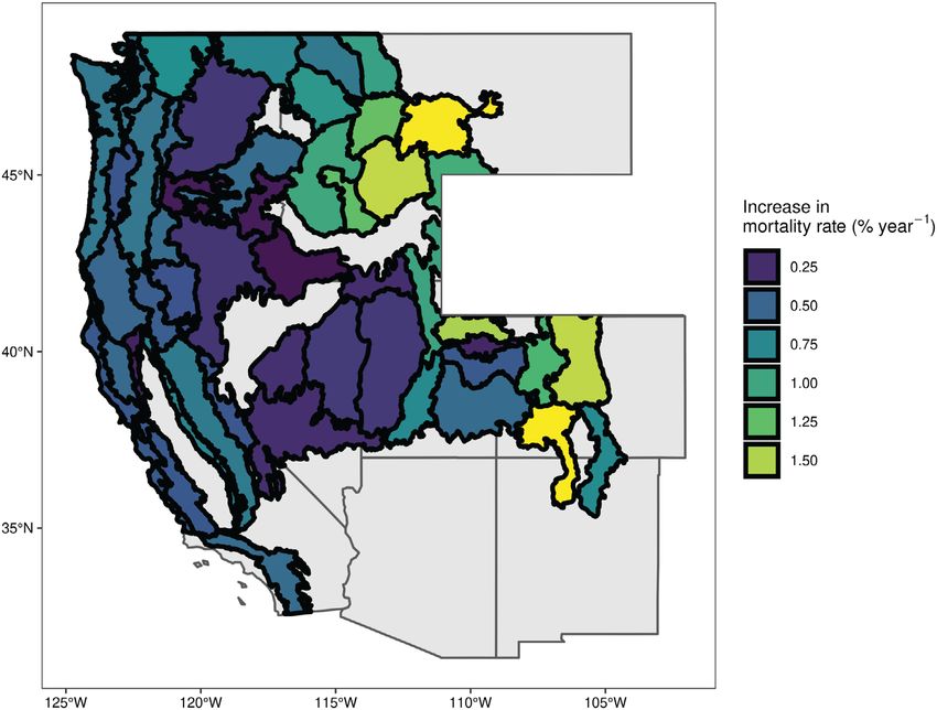
Fig. 1. Map of recent mortality calculated from FIA census data. Mortality rates are calculated over one FIA
census interval and annualized to yearly rates. Polygons outline ecological sections and are colored by mean
recent mortality rate aggregated over all plots within a section (n ≥ 60).
Rocky Mountains and were generally signifi- occurred in the semi-arid sections of the Great
cantly higher than in other regions (Table 1). Spe- Basin and Colorado Plateau and in some sections
cies in these sections with elevated mortality within California. Low mortality rates in the
included Abies lasiocarpa, Populus tremuloides, P. Sierra and Klamath Mountains were driven by
contorta, and Pinus albicaulis, the last of which had low species rates and large sample sizes for Pinus
the highest mortality rate of any species at ponderosa and Abies concolor, with a smaller con-
2.2% yr−1 (Table 2). All sections with >1% mor- tribution from species in the genus Quercus.
tality occurred in the Middle and Southern Notably, some elevated-mortality species occur
Rocky Mountains (Table 1). Sections in the Cas- in regions that did not show high overall forest
cade Mixed Forest Province, generally contigu- mortality, such as Abies magnifica and Quercus
ous with the productive wet temperate forests of gambelii.
the Pacific Northwest, had intermediate mortal- Mortality model prediction accuracy (PCC)
ity rates of between 0.58% and 0.78%. These rates during training was 71.3% with class error rates
were principally driven by the moderate mortal- for alive and dead trees of 27.8% and 29.5%,
ity rates for the dominant conifers Tsuga hetero- respectively. Cohen’s Kappa and the area under
phylla and P. menzeisii at 0.44% and 0.47%, the receiver operating characteristic (AUC) curve
respectively. The lowest recent mortality rates were 0.43 and 0.71, respectively. User’s and
v www.esajournals.org 6 March 2021 v Volume 12(3) v Article e03419MACROSYSTEMS ECOLOGY MCNELLIS ET AL.
Table 1. Recent and future mortality rates (% year−1) for ecological provinces and sections across the western
USA.
Province† Section‡ Recent§ Future¶ Difference#
California Coastal Chaparral Forest and Central California Coast 0.42 1.01 +0.60*
Shruba
California Coastal Range Open Woodlanda Central California Coast Rangesa 0.41 0.84 +0.44NS
California Coastal Range Open Woodland Southern California Mountain andb Valley 0.61 1.73 +1.12**
California Coastal Steppeb Northern California Coast 0.41 0.95 +0.54***
Cascade Mixed Forestc Eastern Cascadesa 0.58 1.54 +0.96***
Cascade Mixed Forest Northern Cascadesb 0.78 2.77 +1.99***
Cascade Mixed Forest Oregon and Washington Coast Rangesb 0.63 2.07 +1.43***
Cascade Mixed Forest Western Cascadesb 0.63 2.28 +1.65***
Intermountain Semi-Desertd Blue Mountain Foothillsa 0.17 0.61 +0.44***
Intermountain Semi-Desert Columbia Basinb 0.28 0.82 +0.53NS
Intermountain Semi-Desert Eastern Basin and Rangeab 0.24 1.05 +0.80*
Intermountain Semi-Desert Northwestern Basin and Rangeab 0.27 0.95 +0.68**
Intermountain Semi-Desert Owyhee Uplandsab 0.15 1.20 +1.05*
Intermountain Semi-Desert and Deserta Bonneville Basina 0.28 1.23 +0.95***
Intermountain Semi-Desert and Desert Monoa 0.52 1.36 +0.84***
Intermountain Semi-Desert and Desert Northern Canyonlandsb 0.58 2.73 +2.15***
Intermountain Semi-Desert and Desert Southeastern Great Basina 0.29 1.01 +0.72***
Intermountain Semi-Desert and Desert Uinta Basinab 0.22 0.57 +0.34NS
Middle Rocky Mountain Steppece Beaverhead Mountainsa 1.51 3.80 +2.29***
Middle Rocky Mountain Steppe Belt Mountainsa 1.74 3.74 +1.99***
Middle Rocky Mountain Steppe Blue Mountainsb 0.56 2.26 +1.71***
Middle Rocky Mountain Steppe Challis Volcanicscd 1.15 4.72 +3.57***
Middle Rocky Mountain Steppe Idaho Batholithc 0.90 3.56 +2.66***
Middle Rocky Mountain Steppe Northern Rockies and Bitterroot Valleyd 1.24 3.52 +2.29***
Nevada-Utah Mountains Semi-Deserta East Great Basin and Mountainsa 0.29 1.52 +1.23***
Nevada-Utah Mountains Semi-Desert Tavaputs Plateaua 0.49 1.8 +1.31***
Nevada-Utah Mountains Semi-Desert Utah High Plateaub 0.81 2.76 +1.95***
Nevada-Utah Mountains Semi-Desert West Great Basin and Mountainsa 0.26 1.34 +1.08***
Northern Rocky Mountain Forest-Steppee Bitterroot Mountainsa 0.87 2.56 +1.69***
Northern Rocky Mountain Forest-Steppe Flathead Valleya 0.68 2.32 +1.64***
Northern Rocky Mountain Forest-Steppe Northern Rockiesa 0.89 3.48 +2.59***
Northern Rocky Mountain Forest-Steppe Okanogan Highlanda 0.75 2.29 +1.54***
Pacific Lowland Mixed Forestb Puget Trougha 0.63 1.69 +1.06***
Pacific Lowland Mixed Forest Willamette Valleyb 0.55 0.97 +0.42**
Sierran Steppeb Klamath Mountainsab 0.51 2.04 +1.53***
Sierran Steppe Modoc Plateauc 0.37 1.21 +0.83***
Sierran Steppe Northern California Coast Rangesad 0.53 1.52 +0.99***
Sierran Steppe Northern California Interior Coast Rangese 0.20 0.52 +0.32NS
Sierran Steppe Sierra Nevadad 0.68 2.08 +1.40***
Sierran Steppe Sierra Nevada Foothillsb 0.89 1.50 +0.61**
Sierran Steppe Southern Cascadesb 0.45 1.04 +0.58***
Southern Rocky Mountain Steppef North Central Highlands and Rocky 1.25 3.31 +2.06***
Mountainsabc
producer’s accuracy for predicting dead trees climate variables (Fig. 2). Diameter of the tree at
was 71.7% and 70.5%, indicating similar errors of the previous inventory, tree maturity index and
omission and co-omission, that is, balanced mod- total plot basal area at the previous inventory
els. Contrary to expectations, model accuracy were more important than all but two climate
was most improved by the inclusion of species variables, although less critical than species iden-
identity and ecological section rather than soil or tity and ecological section. Climate variables of
v www.esajournals.org 7 March 2021 v Volume 12(3) v Article e03419MACROSYSTEMS ECOLOGY MCNELLIS ET AL.
(Table 1. Continued.)
Province† Section‡ Recent§ Future¶ Difference#
Southern Rocky Mountain Steppe Northern Parks and Ranges ad
1.57 3.51 +1.93***
Southern Rocky Mountain Steppe Overthrust Mountainsbe 1.10 3.03 +1.92***
Southern Rocky Mountain Steppe South Central Highlandsd 1.85 3.82 +1.97***
Southern Rocky Mountain Steppe Southern Parks and Rocky Mountain Rangee 0.77 2.37 +1.60***
Southern Rocky Mountain Steppe Uinta Mountainsacd 1.49 3.52 +2.03***
Southern Rocky Mountain Steppe Yellowstone Highlandsbc 1.02 3.55 +2.52***
† Superscripts for provinces show significant differences between province mean mortality rates, where provinces that share
letter groups are not significantly different from one another (Mann–Whitney U-test, α = 0.05). Province names are described
in McNab et al. (2007) and mapped in Cleland et al. (2007).
‡ Superscripts for sections show significant differences in mean mortality rate between sections within a province, where
sections that share letter groups are not significantly different from one another (Mann–Whitney U-test, α = 0.05). Sec-
tion names are described in McNab et al. (2007) and mapped in Cleland et al. (2007).
§ Recent mortality is calculated as plot-level percent mortality over a 10-yr FIA census interval and annualized for yearly
rates.
¶ Future mortality is calculated as plot-level percent mortality from predicted individual tree mortality over a 10-yr FIA cen-
sus interval immediately following the 10-yr recent census interval and annualized for yearly rates.
# Difference in percent mortality between future predicted mortality and recent mortality. Asterisks show statistical signifi-
cance (Mann-Whitney U-test) of with α = 0.05, 0.01, and 0.001 for *, **, and *** respectively. Comparisons with P > 0.05 are
indicated by NS.
importance were largely related to temperature, Juniperus had low overall mortality rates, while P.
especially variables describing the timing and menzeisii had very large sample sizes and are most
severity of frosts (Fig. 2, Appendix S1: Table S1). frequently encountered in regions with low over-
Variables related to water availability were sec- all mortality (Table 2). In contrast to congenerics,
ond to temperature variables, with the most P. ponderosa and Pinus jeffreyi were significantly
important climate variable (summer moisture related to predicting live trees.
index) being strongly related to temperature.
Standard deviations of climate variables were Agent mortality and model performance
much less important than mean values, although Recent mortality rates caused by individual
variables with important means had generally agents averaged from 0.04% yr−1 to 0.28% yr−1,
more important standard deviations. Soil vari- with the highest rates coming from disease
ables were generally unimportant. (0.19% yr−1) and insects (0.28% yr−1) as hypothe-
Important variables contributed unequally to sized. Agent model prediction accuracy during
the probability of assigning a tree as either alive training was 62.8% with class error rates of
or dead (Fig. 3). Species was the strongest contrib- 31.4% (disease), 19.3% (insect), 33.6% (other),
utor in predicting dead trees, with the contribu- 27.3% (vegetation), and 36.3 % (weather).
tion to predicting live trees supported mostly by Cohen’s Kappa was 0.62. User’s accuracy ranged
climate variables related to winter frost and low from 65.9% (weather) to 76.4% (insect) and was
temperatures as well as tree size. Contributions similar to producer’s accuracy, which ranged
were also unequal among species, with contribu- from 63.7% (weather) to 80.3% (insect). Insects
tions to predicting dead trees larger in the genus and disease accounted for 48.7% and 27.3% of
Pinus; P. contorta, P. albicaulis, and Pinus monticola total deaths, respectively. Other and vegetation
especially (Fig. 4). The only other conifers with accounted for 9.2% and 8.0% of total mortality,
significant contribution to predicting dead trees while weather was the least prevalent agent with
were in Abies: A. lasiocarpa, A. lasiocarpa var. arizon- 6.8% of total deaths. Variable importance in the
ica, and A. magnifica. Among hardwoods, P. tremu- agent mortality model was similar to the overall
loides was the third-strongest contributor to mortality model, with species identity (encapsu-
predicting dead trees after the less common Betula lating genetic factors) and ecological section
papyrifera and Chrysolepsis chrysophylla. The most being the two most important variables to
important species for predicting live trees were improving model accuracy (Fig. 5). Climate vari-
principally slow-growing conifers in the genus ables of importance were also similar and gener-
Juniperus along with P. menzeisii and Thuja plicata. ally featured temperature- and frost-related
v www.esajournals.org 8 March 2021 v Volume 12(3) v Article e03419MACROSYSTEMS ECOLOGY MCNELLIS ET AL.
Table 2. Recent and future mortality rates (% year−1) (Table 2. Continued.)
for tree species across the western USA.
Species† Recent‡ Future§ Difference¶
Species† Recent‡ Future§ Difference¶
Tsuga heterophylla 0.44 1.61 +1.17***
Abies amabilis 0.63 2.34 +1.72*** Tsuga mertensiana 0.38 1.74 +1.36***
Abies concolor 0.73 2.56 +1.84*** Umbellularia californica 0.22 0.39 +0.17NS
Abies grandis 0.72 2.51 +1.79*** † Species identity and taxonomic information are found in
Abies lasiocarpa 0.93 4.38 +3.46*** Burril et al. (2018), Appendix F.
Abies lasiocarpa var. 2.72 5.89 +3.18*** ‡ Recent mortality is calculated as species-level percent
arizonica mortality over a 10-yr FIA census interval and annualized to
Abies magnifica 0.90 3.67 +2.77*** yearly rates.
§ Future mortality is calculated as species-level percent
Abies procera 0.43 1.51 +1.08NS mortality from predicted individual tree mortality and annu-
Abies shastensis 0.75 2.91 +2.16*** alized to yearly rates.
Acer grandidentatum 0.41 1.17 +0.77*** ¶ Difference in percent mortality between future predicted
Acer macrophyllum 0.45 0.71 +0.27NS mortality and recent mortality. Asterisks show statistical sig-
nificance (Mann–Whitney U-test) with α = 0.05, 0.01, and
Alnus rubra 1.15 1.67 +0.52***
0.001 for *, **, and *** respectively. Comparisons with
Arbutus menziesii 0.77 1.91 +1.14*** P > 0.05 are indicated by NS.
Betula papyrifera 2.17 5.59 +3.42***
Calocedrus decurrens 0.42 1.55 +1.13***
Cercocarpus ledifolius 0.36 2.98 +2.62*** variables. Notably, minimum zero-degree-days
Chamaecyparis lawsoniana 0.30 4.25 +3.95*** was an important feature for reducing model
Chamaecyparis nootkatensis 0.11 2.60 +2.49*** error in the agent mortality model (7th most
Chrysolepis chrysophylla 0.97 3.11 +2.14*** important) but not important for reducing model
var. chrysophylla
error in the overall mortality model (25th most
Juniperus monosperma 0.08 1.77 +1.69***
Juniperus occidentalis 0.04 0.29 +0.25NS important). Additionally, the standard deviation
Juniperus osteosperma 0.03 1.03 +1.00*** of zero-degree-days was very important for
Juniperus scopulorum 0.06 0.99 +0.93*** agent mortality and was the only climate vari-
Larix occidentalis 0.60 2.93 +2.33*** ability feature to be one of the 15 most-valuable
Lithocarpus densiflorus 0.39 0.43 +0.04** features in either model (Figs. 2, 5).
Picea engelmannii 1.44 2.84 +1.40*** Variables did not contribute equally to the
Picea pungens 0.43 1.43 +1.00***
probability of predicting dead or live trees across
Picea sitchensis 0.59 2.69 +2.10***
Pinus albicaulis 2.20 5.84 +3.63** all mortality agents (Fig. 5, Table 3). Variables
Pinus aristata 0.40 3.96 +3.56*** that contributed strongly to predicting trees
Pinus contorta 2.03 3.64 +1.61*** killed by insect were total zero-degree-days
Pinus edulis 0.36 1.61 +1.24*** based on minimum temperatures (+0.93%), mini-
Pinus flexilis 1.29 4.54 +3.25*** mum temperature of the coldest month
Pinus jeffreyi 0.24 0.70 +0.47NS (+1.13%), and specific humidity (+0.66%;
Pinus lambertiana 0.87 2.81 +1.94***
Table 3). Specific humidity also contributed to
Pinus monophylla 0.37 0.98 +0.61***
Pinus monticola 1.28 4.57 +3.29*** predicting disease deaths (+0.26%), but so did
Pinus ponderosa 0.43 0.91 +0.48*** owner group code (+0.22%). Interestingly, no
Pinus sabiniana 0.57 0.48 -0.09NS precipitation variables contributed to predicting
Populus balsamifera ssp. 0.65 1.76 +1.11** dead trees of any mortality agent (Table 3). Mor-
trichocarpa
tality from weather was only predicted by the
Populus tremuloides 1.86 4.16 +2.29***
Pseudotsuga menziesii 0.47 1.96 +1.49***
length of the frost-free period (+0.17%) and local
Quercus agrifolia 0.73 1.09 +0.37* physiographic class (+0.25%). The only variable
Quercus chrysolepis 0.2 0.44 +0.24* with a greater than 0.05% contribution to predict-
Quercus douglasii 0.34 0.55 +0.21NS ing vegetation mortality was species (+0.18%).
Quercus gambelii 0.82 2.12 +1.30***
Quercus garryana 0.41 0.92 +0.51* Tree mortality across the western USA under
Quercus kelloggii 0.62 1.45 +0.83***
future climates
Quercus wislizeni 0.8 1.49 +0.69***
Sequoia sempervirens 0.09 0.96 +0.87*
Forest mortality across the study area was pre-
Thuja plicata 0.12 1.43 +1.30*** dicted to increase in most regions with the largest
magnitude increases in the Southern and Middle
v www.esajournals.org 9 March 2021 v Volume 12(3) v Article e03419MACROSYSTEMS ECOLOGY MCNELLIS ET AL.
Fig. 2. Feature importance for the overall mortality model. Units for each feature are given in Appendix S1:
Table S1. Variables are sorted according to their contribution to the decrease in overall model accuracy when they
are excluded from mortality predictions. Variables are colored according to their source: Dark gray location vari-
ables are sourced or derived from plot- or tree-level FIA data, light gray soil variables are sourced from 250 m
SoilGrids soils data, and black climate variables are sourced or derived from gridMET and MACA gridded cli-
mate data sets.
v www.esajournals.org 10 March 2021 v Volume 12(3) v Article e03419MACROSYSTEMS ECOLOGY MCNELLIS ET AL.
Fig. 3. Median contribution of each Random Forest feature to the probability of positively identifying a tree
that died during the census interval (y > 0) when assessed over the entire forest of classification trees. Units on
the y-axis are decimal probability.
Rocky Mountains (+2.02−2.52% yr−1, Fig. 6, Fig. 7). Broader patterns in future rates for
Table 1). Species-specific effects (including genetic genera were visible, including low future rates for
effects) were most important to future mortality Juniperus and Quercus and high future rates for
rates and were inflated by increases in mortality Pinus (Table 2). However, no genus represented
for some species of up to 3.63% yr−1, including P. by multiple species was significantly more or
albicaulis (+3.63%), P. contorta (+1.61%), A. lasio- less vulnerable overall than another. Pinus
carpa (+3.46%), A. lasiocarpa var. arizonica ponderosa and Pinus jeffreyi were notable outliers
(+3.18%), and P. tremuloides (+2.29%, Table 2). within Pinus, with a less than 0.5% predicted
Only one species, Pinus sabiana, had a non-statisti- increase (Table 2). Mortality rates increased
cally significant decrease in mortality rates under substantially under future climates for all agents
future climates. Recent mortality at the plot level up to more than 0.6% yr−1 for disease and
was not correlated with future mortality but Insect (Fig. 8). The proportion of trees killed by
showed a strong correlation by species (r2 = 0.59; insect dropped from 48.6% to 27.6% and was
v www.esajournals.org 11 March 2021 v Volume 12(3) v Article e03419MACROSYSTEMS ECOLOGY MCNELLIS ET AL.
Fig. 4. Partial dependence of dead tree predictions on the species of the individual tree, when all other vari-
ables are controlled for. Units on the y-axis are expressed as the logit of the probability of predicting a dead tree,
with 0 representing an equal contribution to predicting alive and dead trees.
accompanied by increases in all other categories identity was overwhelmingly our most impor-
(Fig. 8). tant predictor variable, which demonstrates the
important influence of genetics on tree mortality
DISCUSSION (Rehfeldt et al. 2006). Although beyond the scope
of this study, the significant contribution of spe-
Factors most important to recent and future cies identity to our mortality predictions war-
forest mortality rants more careful consideration of the influence
Our results report on recent mortality rates for that genetics may have on overall tree mortality
many western U.S. forests and attempt to eluci- as well as how cause of death may vary between
date the important drivers of mortality in these species subpopulations (Rehfeldt et al. 2006).
systems. Previous work on forest mortality has We found that large tree mortality in the west-
largely focused on catastrophic mortality from ern USA is likely to accelerate under future cli-
drought, fire, and insects, and we therefore mate regimes, in general agreement with other
hypothesized that the most important predictors studies (Dale et al. 2001, Allen et al. 2010). This
of both recent and future mortality would be result supports our hypothesis of increased mor-
environmental variables associated with precipi- tality under future climates, but drivers of these
tation and temperature (Berner et al. 2017, Fettig increases may be nuanced. Specifically, the
et al. 2019). Rather than climate or soil, species importance of species identity in model
v www.esajournals.org 12 March 2021 v Volume 12(3) v Article e03419MACROSYSTEMS ECOLOGY MCNELLIS ET AL.
Fig. 5. Feature importance for the agent mortality model. Units for each feature are given in Appendix S1:
Table S1. Variables are sorted according to their contribution to the decrease in overall model accuracy when they
are excluded from predictions. Variables are colored according to their source: Dark gray location variables are
sourced or derived from plot- or tree-level FIA data, light gray soil variables are sourced from 250 m SoilGrids
soils data, and black climate variables are sourced or derived from gridMET and MACA gridded climate data
sets.
performance suggests that these changes will be variability in future mortality rates suggests that
heavily dependent on species and ecosystem. In predicting how these forests change in the future
support of this, future mortality was not corre- will require detailed knowledge of how vulnera-
lated with past mortality at the plot level but ble species respond to environmental drivers.
showed a strong dependence on species. Large Perhaps more importantly, detailed empirical
v www.esajournals.org 13 March 2021 v Volume 12(3) v Article e03419MACROSYSTEMS ECOLOGY MCNELLIS ET AL. Table 3. Median contribution of each feature to the probability of positively identifying a tree killed by insects, disease, weather, vegetation, or other when assessed over the entire forest of classification trees. Feature Insect Disease Weather Vegetation Other Absolute depth to bedrock −0.02 −0.07 −0.06 −0.04 −0.07 Accu. precipitation, April–September −0.04 −0.06 −0.12 −0.03 −0.05 Accu. precipitation, April–September, SD −0.1 −0.07 −0.08 −0.06 −0.03 Accumulated precipitation −0.14 −0.07 −0.14 −0.12 −0.06 Accumulated precipitation, SD −0.23 −0.09 −0.08 −0.1 −0.08 Annual moisture index −0.01 −0.04 −0.09 −0.03 −0.06 Annual moisture index, SD −0.01 −0.05 −0.08 −0.03 −0.07 Average temperature in the coldest month −0.78 −0.04 0.06 −0.36 0.03 Average temperature in the coldest month, SD −0.01 −0.06 −0.07 −0.03 −0.08 Average temperature in the warmest month −0.04 −0.04 −0.05 −0.02 −0.11 Average temperature in the warmest month, SD −0.04 −0.05 −0.04 −0.03 −0.05 Bulk density fine earth −0.02 −0.06 −0.12 −0.11 −0.07 Cation exchange capacity of soil −0.03 −0.03 −0.11 −0.09 −0.05 Clay content mass fraction 0.02 −0.18 −0.03 −0.05 −0.11 Degree-days 5°C, SD −0.05 −0.06 −0.06 −0.05 −0.06 Day of year of the first freezing date of autumn −0.6 −0.16 0.07 −0.11 −0.03 Day of year of the first freezing date of autumn, SD −0.02 −0.07 −0.06 −0.04 −0.08 Day of year of the last freezing date of spring −0.64 −0.13 0.06 −0.05 −0.04 Day of year of the last freezing date of spring, SD −0.03 −0.06 −0.03 −0.02 −0.07 Day of year when sum of degree-days >5°C reaches 100 −0.24 −0.05 −0.02 −0.06 −0.02 Day of year when sum of degree-days >5°C reaches 100, SD −0.02 −0.03 −0.02 −0.02 −0.02 Length of frost-free period −0.95 −0.13 0.17 −0.12 −0.03 Length of frost-free period, SD −0.03 −0.07 −0.04 −0.03 −0.06 Local physiographic class −0.02 −0.05 0.25 −0.03 0.14 Maximum temperature −0.14 −0.07 −0.03 −0.03 −0.11 Maximum temperature in the warmest month −0.02 −0.04 −0.06 −0.03 −0.08 Maximum temperature in the warmest month, SD −0.03 −0.05 −0.04 −0.02 −0.1 Maximum temperature, SD −0.02 −0.04 −0.08 −0.01 −0.04 Minimum degree-days
MACROSYSTEMS ECOLOGY                                                                                     MCNELLIS ET AL.

(Table 3. Continued.)

Feature                                                           Insect     Disease      Weather        Vegetation   Other

Sum of >5°C degree-days within the frost-free period, SD          −0.03       −0.05         −0.05          −0.04      −0.06
Summer moisture index                                             −0.03       −0.06         −0.08          −0.03      −0.08
Summer moisture index, SD                                           0         −0.13           0             0.02      −0.21
Summer–winter temperature differential                            0.23         0.05         −0.23          −0.47       0.01
Summer–winter temperature differential, SD                        −0.02       −0.06         −0.05          −0.03      −0.05
Topographic solar-radiation index                                 −0.01       −0.04         −0.05          −0.03      −0.08
Tree diameter at previous census                                  −0.05       −0.18         −0.19             0       −0.17
Tree maturity index                                               −0.01        0.12         −0.07          −0.37       0.02
Volumetric coarse fragments                                       −0.03       −0.08         −0.08          −0.04      −0.05
Wind speed                                                        −0.03       −0.03         −0.07          −0.03      −0.08
Wind speed, SD                                                    −0.01       −0.03         −0.06          −0.01      −0.16
  Notes: Units are decimal probability × 102. Standard deviation of climate variables is indicated with an SD.

data on demographic changes to U.S. forests will                  white pine blister rust as major contemporary
be needed across large geographic areas and                       disturbances throughout the range of these spe-
over decadal time periods.                                        cies (Geils et al. 2010, Jacobi et al. 2018). Alterna-
   Species-specific life-history traits, especially                tively, some species or populations may
tree age, likely contributed heavily to mortality                 currently be in the midst of a widespread die-
predictions. This was supported by unequal spe-                   back due to anthropogenic climate change that is
cies contributions to predicting mortality as well                pushing them past critical environmental stress
as significant variability in observed and pre-                    tolerance thresholds despite apparently normal
dicted mortality rates (Fig. 4, Table 2). While tree              mortality for the ecosystem or region (Huang
age itself may not be directly impacting mortality                et al. 2015, Kolb 2015). Our results somewhat
through age-related senescence, low stem turn-                    agree with previous work that suggests future
over in long-lived trees complicates interpreta-                  forest mortality may be a widespread phe-
tion between some of our species. For example,                    nomenon, but we emphasize that some species
relatively high mortality rates may be normal for                 and regions may be disproportionately affected
some short-lived (~100 yr) early successional                     (Allen et al. 2010, Kane et al. 2014, McDowell
species such as A. rubra or P. tremuloides (Har-                  and Allen 2015). Future efforts to mitigate the
rington et al. 1994, Mitton and Grant 1996). Con-                 effects of anthropogenic climate change should
versely, long-lived tree species such as P.                       focus on active management or conservation of
menzeisii or members of Juniperus may live more                   key species or populations, and future efforts to
than 1000 yr and may not die for some time after                  model mortality risk in western U.S. forests
the onset of lethal environmental or biotic stress                should emphasize plant functional traits or phys-
(Alexander et al. 2018). Differences in life-history              iology common to vulnerable species, such as
traits may partly be responsible for the strong                   current efforts to control white pine blister rust
dependence of mortality predictions on species                    in P. monticola and P. albicaulis (Geils et al. 2010,
identity but seem unlikely to contribute to our                   Jacobi et al. 2018).
predictions of mortality under future climates. In                   We assessed mortality rates for some well-
support of this, we found that our maturity index                 studied tree species and many other tree species
variable was the 4th most important variable for                  that, to our knowledge, do not have any pub-
reducing model error in our first mortality model                  lished mortality rates. The most common focal
and contributed significantly to predicting live                   conifer species in recent mortality work have
trees. Other important life-history traits may                    been conifers in the genera Abies, Pinus, and
include vulnerability to host-specific pathogens                   Juniperus (Gaylord et al. 2013, Krofcheck et al.
—P. monticola and P. albicaulis; for example, both                2014, Mortenson et al. 2015, Fettig et al. 2019,
had high recent and future mortality rates and                    Flake and Weisberg 2019, Pile et al. 2019,
previous research implicates bark beetles and                     McDowell et al. 2019). We improve on previous

                 v www.esajournals.org                       15              March 2021   v Volume 12(3) v Article e03419
MACROSYSTEMS ECOLOGY MCNELLIS ET AL.
Fig. 6. Map of differences in mortality rate between recent forest mortality and mortality predicted under the
RCP 4.5 emissions scenario. Polygons outline ecological sections and are colored by mean difference in mortality
rate aggregated over all plots within a section.
mortality research for these species by including on specific mortality events, localized to one for-
populations over wide areas, as well as including est or region. For example, Worrall et al. (2008)
species closely related to common focal species found mortality rates of ~11% yr−1 in four stands
that are less well studied. Future research should of P. tremuloides in Colorado, but this was in an
incorporate these species to improve modeling area of highly concentrated aspen mortality. Pre-
efforts and inform forest managers and policy- dicted future mortality rates were significantly
makers. higher than recent rates as well as some future
Arguably the most well-studied forest dieback rates predicted by other studies. For example,
is the recent widespread decline of quaking Rehfeldt et al. (2009) used Random Forest to pre-
aspen, P. tremuloides (Rehfeldt et al. 2009, Worrall dict bioclimate envelopes for P. tremuloides and
et al. 2010, Huang and Anderegg 2012, Anderegg suggested a decrease of 6–41% in available envel-
et al. 2013, Tai et al. 2017). Despite being one of ope area by 2030, a 0.3–2% yr−1 mortality rate
the highest recent mortality rates observed in our that contrasts with our projected future rate of
dataset, our mean rate of 1.86% yr−1 was less 4.16% yr−1 (Table 2). Nonetheless, P. tremuloides
than mortality rates observed in other studies. will likely be one of the most at-risk western U.S.
Part of this may be due to the spatial extent of tree species under future climates and may face
plots in our dataset—other studies tend to focus significant local and regional risk of extirpation
v www.esajournals.org 16 March 2021 v Volume 12(3) v Article e03419MACROSYSTEMS ECOLOGY MCNELLIS ET AL.
modeled estimates for a more robust assessment
of emerging risks to western U.S. forests (Meir
et al. 2015).
Our recent mortality rates are generally lower
than previously published rates for other less
well-studied species. For example, Mortenson
et al. (2015) reported mortality rates in the Kla-
math range for A. magnifica, P. jeffreyi, P. contorta,
and A. concolor as 1.8% yr−1, 1.9% yr−1, 1.1%
yr−1, and 3.0% yr−1, respectively, compared with
0.90% yr−1, 0.24% yr−1, 2.03% yr−1, and 0.72%
yr−1 for the same species in this study. Our exclu-
sion of fire as a mortality agent probably lowers
our estimated and predicted rates for species in
fire-prone ecosystems such as the Klamath range
(Hagmann et al. 2013). However, we can extend
this work by noting that mortality rates are likely
to increase even further, especially for A. mag-
nifica (+3.66%) and P. contorta (+3.64%).
Fig. 7. Scatterplot of recent mortality rates versus
The partial dependence of species on predict-
future mortality for 53 large tree species across the
ing live trees suggested some species that may be
western USA; P < 0.01, r2 = 0.59. The thin gray line
less vulnerable under future climates, including
represents a 1:1 reference between recent and future
P. ponderosa and members of the genus Juniperus
mortality rates.
or Quercus. While P. ponderosa in this study
showed a small increase in mortality rates rela-
tive to congenerics, other studies have observed
dramatic P. ponderosa mortality from drought
events at the southern end of its range (Allen and
Breshears 1998). These species may serve as good
models or keystone species when examining
future forest dieback—diebacks at low latitudes
or low elevations may portend similar events at
high latitudes or high elevations (Aitken et al.
2008). Alternatively, shifts in the distribution and
abundance of these species due to climate change
may occur in younger cohorts or in conjunction
with disturbance events such as fire (Kemp et al.
2019). Future work on forest mortality would
benefit from examining whole-range demo-
graphics of these species, especially in the con-
text of plant functional traits or population
genetics measured throughout a species range
(Rehfeldt et al. 2006).
Fig. 8. Recent and future mortality rates for five Juniper mortality increased only moderately
mortality agent classes. Bars are mean rates across under future climates in this study, confirming
plots expressed as annualized plot mortality 1 SE. previous work that suggests that juniper is
robust to die-off events (Table 2; Floyd et al.
(Aitken et al. 2008). To reconcile differences in 2009). A significant body of work suggests that
the magnitude of predicted mortality for P. in these systems, Pinus edulis, P. monophylla, and
tremuloides, future research should utilize empiri- P. ponderosa may have elevated-mortality rates
cal predictions of future mortality as well as under future climates. Interestingly, our
v www.esajournals.org 17 March 2021 v Volume 12(3) v Article e03419MACROSYSTEMS ECOLOGY MCNELLIS ET AL.
predicted increases in mortality rates are much describing the timing and severity of winter tem-
smaller in magnitude than other studies observ- peratures (Figs. 2, 5). Changes to winter temper-
ing Pinus die-off events. This is probably because atures as a result of anthropogenic climate
our rates reflect mortality dynamics aggregated change may influence tree mortality rates, espe-
throughout the species’ entire range, in contrast cially at high latitudes or at high elevations such
to other studies that focus on mortality at their as those in the Rocky Mountains. Furthermore,
edges (e.g., Allen and Breshears 1998). Future increases in warm-season temperature may
work should focus on the consequences of these increase tree mortality through increased vapor-
marginal die-off events for Juniperus, for exam- pressure deficit and mortality from drought
ple, type conversion to smaller-statured wood- stress (Park Williams et al. 2013). Interestingly,
land or shrubland or loss of ecosystem services water availability variables were much less influ-
such as carbon storage. ential in predicting mortality despite the strong
influence of precipitation on forest structure
Other factors driving recent tree mortality and throughout the western USA. Some previous
mortality agents across the western USA research suggests that temperature has a strong
Tree diameter was the 3rd most important relationship with tree drought stress due to its
variable for improving model accuracy and con- contribution to vapor-pressure deficit (Adams
tributed significantly to predicting alive trees. et al. 2017), indicating that increased air tempera-
Larger, longer-lived trees may be less vulnerable ture may have a direct influence on tree mortality
to density-dependent mortality effects from com- independent of future changes to precipitation
petition for water or nutrients (Luo and Chen regimes. Combined with our results here, this
2011, Harmon and Pabst 2015). This is supported may indicate that Rocky Mountain forests may
by our finding that tree maturity and plot basal be disproportionately affected by drier, warmer
area at either inventory were important for pre- temperatures, even when compared to other
dicting live trees, although maturity was much regions in the western USA.
less important overall to reducing model error. One potential explanation for the connection
Nonetheless, tree size alone was not enough to between winter frosts and forest mortality is
account for observed mortality rates and was the influence of snowpack. While we did not
unlikely to be responsible for increases in mortal- include measures of snowpack in our analysis,
ity in the future (Uriarte et al. 2004, Zhang et al. significant previous research has suggested that
2013, Birch et al. 2015). changes to snowpack volume may be critical in
Ecological section was very important for determining drought stress in montane envi-
improving model accuracy but did not con- ronments (Anderegg et al. 2013). Alternatively,
tribute to dead tree predictions more than live winter frosts may be influencing forest mortal-
trees. This suggests that recent mortality rates in ity by mediating the relationship between
the absence of catastrophic disturbance may be insect outbreak and tree death (Weed et al.
further dependent on spatially correlated vari- 2013). Previous research suggests mild winter
ables that were not included in this dataset. Sec- temperatures and moderate rainfall contribute
tions are defined as an aggregate of geologic, most to insect outbreak risk (Sidder et al. 2016).
soil, and vegetative properties and may include Currently, the effect of insects on tree mortality
qualitative descriptors that do not continuously is difficult to model and many ecosystem and
vary along grids (McNab et al. 2007). While earth system models do not explicitly include
major improvements to modeling forest mortal- insect effects. The relationship between temper-
ity may involve species-specific parameteriza- ature and tree death may be greatly enhanced
tions, variation in demographic rates across in models of mortality if the more immediate
space and between tree populations may present effects on snowpack and insect populations are
an additional challenge that may require detailed more carefully considered (Ayres and Lom-
knowledge of tree eco-physiology (Bohner and bardero 2000).
Diez 2020). Soil variables were relatively unimportant for
The most important climate variables were predicting mortality across this dataset and con-
related to temperature, especially variables tributed little to predicting alive or dead trees
v www.esajournals.org 18 March 2021 v Volume 12(3) v Article e03419MACROSYSTEMS ECOLOGY MCNELLIS ET AL.
(Figs. 2, 3). The two most important variables irregular inventory data prior to 2000 may be sig-
were bulk density of the fine earth element and nificantly less reliable in assessing forest dynam-
available water-holding capacity. Both may be ics (Goeking 2015).
related to drought tolerance, water, or nutrient A potential source of error in our analysis
availability through competition for below- comes from the fuzzing and swapping of plot
ground resources, although root competition is coordinates on tribal and privately owned lands
generally less important for trees than for grasses (Tinkham et al. 2018). Plot coordinates in pub-
or forbs (Casper and Jackson 1997, Sperry et al. licly available FIA data are reported up to 1 km
1998, Kiaer et al. 2013). Our results suggest little away from their true locations in order to pre-
influence of soil variability on tree mortality, vent vandalism and to preserve the confidential-
although soils may exert indirect control on tree ity of private landowner data (Tinkham et al.
demographics through other mechanisms such 2018). Additionally, 20% of plot coordinates
as habitat filtering (Kraft et al. 2015). located on private land are swapped with other
plot coordinates within the same county (Burrill
Implications for future work examining forest et al. 2018). While this process may significantly
mortality influence some spatial analyses, the high spatial
The strong influence of species identity on autocorrelation of our gridded independent vari-
reducing error in the predictive model indicates ables (both climate and soil variables), smaller
that current attempts to model forest mortality contribution from plots on private land, and non-
will likely require extensive parameterization at parametric analysis likely reduced error from
the species or functional group level, even if gen- plot perturbation well below other sources of
eral plant eco-physiology is faithfully repre- variability within the dataset (Coulston et al.
sented in model processes (Adams et al. 2013, 2006).
Meir et al. 2015). Buotte et al. (2019) recently Our analysis of mortality agents in FIA has sig-
accomplished this by expanding the single ever- nificant limitations. Specifically, the limited reso-
green functional type utilized in a large earth lution on causes of mortality in our dataset
system model to 13 functional types that repre- precludes strong conclusions about future mor-
sent more distinct forest ecosystems. Conse- tality for some species and regions. This issue is
quently, they reported significant improvements made worse by the subjectivity often associated
in model performance. While parameterizing an with assigning a causal agent in the field up to
earth system model for 53 species is no doubt several years after a tree has died (e.g., Bigler
challenging in some studies, careful selection of et al. 2007). Some causal agents such as drought
species to include may put upper and lower stress may not be immediately visible to field
bounds on the impact that climate change will technicians as a proximate cause of death, and
have on western forests. Alternatively, new without detailed physiological measurements we
advances in earth system models could more cannot know for certain what killed a tree that
explicitly link models to trait databases, allowing we observed dead. Future work utilizing FIA
rapid evaluation of many species simultaneously data would benefit from a more robust under-
(Kattge et al. 2011). standing of the limitations imposed by FIA mor-
tality agent methodology, including limits posed
Methodological caveats and considerations by on-the-ground accuracy that are independent
We deliberately chose to use FIA data collected of field technician training.
since 2000. Specifically, we restricted our analysis In this study, we specifically excluded harvest
to trees measured under the National Plot Design and fire mortality because of their disconnect
to improve the reliability and accuracy of our with ultimate causes of mortality at the tree
mortality estimates. While tree records before level. Nonetheless, both are major sources of
2000 are available from FIA, mortality as a demo- mortality within all forested systems in our
graphic process is most robustly assessed using study area (Berner et al. 2017). Commercial tree
individual tree tracking that did not begin until harvest is a primary cause of mortality in sec-
the National Plot Design (Smith 2002). Addition- tions within the Cascade Mixed Forest and
ally, previous work has suggested that the likely disrupts climate-driven demographic
v www.esajournals.org 19 March 2021 v Volume 12(3) v Article e03419You can also read