The incorporation of the Tripleclouds concept into the δ-Eddington two-stream radiation scheme: solver characterization and its application to ...
←
→
Page content transcription
If your browser does not render page correctly, please read the page content below
Atmos. Chem. Phys., 20, 10733–10755, 2020
https://doi.org/10.5194/acp-20-10733-2020
© Author(s) 2020. This work is distributed under
the Creative Commons Attribution 4.0 License.

The incorporation of the Tripleclouds concept into the δ-Eddington
two-stream radiation scheme: solver characterization and its
application to shallow cumulus clouds
Nina Črnivec1 and Bernhard Mayer1,2
1 Chair   of Experimental Meteorology, Ludwig-Maximilians-Universität München, Munich, Germany
2 Institut für Physik der Atmosphäre, Deutsches Zentrum für Luft- und Raumfahrt, Oberpfaffenhofen, Germany

Correspondence: Nina Črnivec (nina.crnivec@physik.uni-muenchen.de)

Received: 7 April 2020 – Discussion started: 30 April 2020
Revised: 13 July 2020 – Accepted: 24 July 2020 – Published: 14 September 2020

Abstract. The treatment of unresolved cloud–radiation in-          tion. Whereas previous studies employing the Tripleclouds
teractions in weather and climate models has considerably          concept focused on researching the top-of-the-atmosphere
improved over the recent years, compared to conventional           radiation budget, the present work applies Tripleclouds to
plane-parallel radiation schemes, which previously persisted       atmospheric heating rate and net surface flux. The Triple-
in these models for multiple decades. One such improvement         clouds scheme was implemented in the comprehensive li-
is the state-of-the-art Tripleclouds radiative solver, which has   bRadtran radiative transfer package and can be utilized to
one cloud-free and two cloudy regions in each vertical model       further address key scientific issues related to unresolved
layer and is thereby capable of representing cloud horizon-        cloud–radiation interplay in coarse-resolution atmospheric
tal inhomogeneity. Inspired by the Tripleclouds concept, pri-      models.
marily introduced by Shonk and Hogan (2008), we incor-
porated a second cloudy region into the widely employed
δ-Eddington two-stream method with the maximum-random
overlap assumption for partial cloudiness. The inclusion of        1   Introduction
another cloudy region in the two-stream framework required
an extension of vertical overlap rules. While retaining the        Radiation schemes in coarse-resolution numerical weather
maximum-random overlap for the entire layer cloudiness,            prediction and climate models, commonly referred to as
we additionally assumed the maximum overlap of optically           general circulation models (GCMs), have traditionally been
thicker cloudy regions in pairs of adjacent layers. This ex-       claimed to be impaired by the poor representation of clouds
tended overlap formulation implicitly places the optically         (Randall et al., 1984, 2003, 2007). Undoubtedly, one of the
thicker region towards the interior of the cloud, which is in      most rigorous assumptions that persisted in GCMs for mul-
agreement with the core–shell model for convective clouds.         tiple decades, was the complete removal of cloud horizontal
The method was initially applied on a shallow cumulus cloud        heterogeneity – the so-called plane-parallel cloud represen-
field, evaluated against a three-dimensional benchmark radi-       tation (Fig. 1d). Since the nature of cloud–radiation interac-
ation computation. Different approaches were used to gener-        tions is intrinsically nonlinear, the plane-parallel representa-
ate a pair of cloud condensates characterizing the two cloudy      tion of clouds leads to substantial biases of GCM radiative
regions, testing various condensate distribution assumptions       quantities (Cahalan et al., 1994a, b; Cairns et al., 2000). Fur-
along with global cloud variability estimate. Regardless of        ther, an assumption of how partial cloudiness vertically over-
the exact condensate setup, the radiative bias in the vast ma-     laps within each GCM grid column is required. The widely
jority of Tripleclouds configurations was considerably re-         employed assumption is the maximum-random overlap (Ge-
duced compared to the conventional plane-parallel calcula-         leyn and Hollingsworth, 1979), advocated by many studies
                                                                   (e.g., Tian and Curry, 1989) and recently criticized by oth-

Published by Copernicus Publications on behalf of the European Geosciences Union.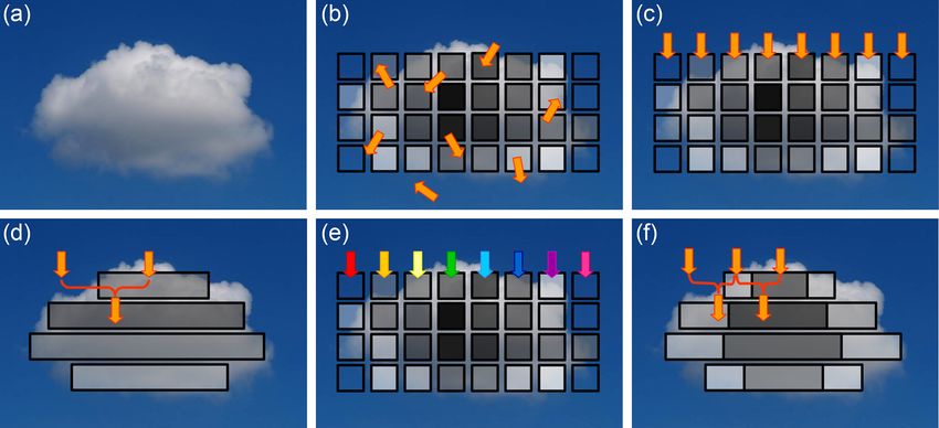
10734                   N. Črnivec and B. Mayer: The Tripleclouds method and its application to shallow cumulus clouds

ers, since it breaks down in the case of vertically developed        nen et al. (2005) for global climate simulated with another
cloud systems in strongly sheared environments (e.g., Hogan          GCM.
and Illingworth, 2000; Naud et al., 2008; Di Giuseppe and               A few years after the introduction of the McICA, Shonk
Tompkins, 2015). Last but not least, three-dimensional (3-D)         and Hogan (2008) (hereafter abbreviated as SH08) proposed
radiative effects related to subgrid horizontal photon trans-        a unique method which utilizes two regions in each verti-
port, which in reality manifests itself most pronouncedly in         cal model layer to represent the cloud, as opposed to one.
regions characterized by strong horizontal gradients of op-          One region is used to represent the optically thicker part of
tical properties, such as cloud side boundaries (Jakub and           the cloud and the other represents the remaining optically
Mayer, 2015, 2016; Klinger and Mayer, 2014, 2016), are cur-          thinner part; the method therefore captures cloud horizon-
rently still neglected in the majority of GCMs. This broad           tal inhomogeneity. Together with the cloud-free region, the
palette of issues is challenging to tackle and solve.                radiation scheme thus has three regions at each height and
    In order to reduce the most striking plane-parallel biases,      is referred to as the “Tripleclouds” (TC) scheme. In the pri-
several methods were developed in the past. The scaling fac-         mary work of SH08, the layer cloudiness was split into two
tor method, proposed by Cahalan et al. (1994a) and imple-            equally sized regions and the corresponding pair of cloud
mented in the ECMWF model by Tiedtke (1996), was a con-              condensates (e.g., liquid water content; LWC) was generated
ventional approach, where the cloud optical depth was mul-           on the basis of known LWC distribution. The method was
tiplied by a constant factor and the resulting effective opti-       initially tested on high-resolution radar data, where the ex-
cal depth was passed to the radiation scheme. Oreopoulos et          act position of the three regions was passed to the radiative
al. (1999) introduced a more sophisticated gamma-weighted            solver, capable of representing an arbitrary vertical overlap.
radiative transfer scheme, later also applied by Carlin et al.       In practice, a host GCM usually provides only mean LWC
(2002) and Rossow et al. (2002), where the optical depth             and no information about vertical cloud arrangement. In or-
across a grid box is weighted using a gamma distribution.            der to make the method applicable to GCMs, Shonk et al.
Moreover, Barker et al. (2002) and subsequently Pincus et            (2010) derived a global estimate of cloud horizontal variabil-
al. (2003) presented an alternative technique, known as the          ity in terms of fractional standard deviation (FSD), which
Monte Carlo integration of independent column approxima-             can be used to split the mean LWC into two components
tion (McICA; Fig. 1e), which is currently operationally em-          along with the LWC distribution assumption. Further, they
ployed in most large-scale atmospheric models. The funda-            incorporated a generalized vertical overlap parameterization,
mental assumption of the McICA is that the independent               called the exponential-random overlap, accounting for the
column approximation (ICA; Fig. 1c) is adequate and there-           aforementioned problematics in strongly sheared conditions.
fore allows for the independent generation of subgrid cloudy         Recently, the method was successfully implemented in the
columns, which is managed by means of stochastic cloud               ecRad package (Hogan and Bozzo, 2018), the current radi-
generator (Räisänen et al., 2004; Räisänen and Barker, 2004).        ation scheme of ECMWF Integrated Forecast System (IFS).
As the full ICA is not affordable within the computational           In contrast to the McICA, which is still operational also at
constraints of simulating complex weather and climate sce-           ECMWF due to its higher computational efficiency, the TC
narios, the computing speed gain in the McICA approach is            scheme does not produce any radiative noise. As suggested
based on the simultaneous sampling of subgrid cloud state            by Hogan and Bozzo (2016), this superiority could become
and spectral interval.                                               even more valuable in the future if an alternative gas optics
    Whereas all aforementioned methodologies certainly               model with fewer spectral intervals than the current Rapid
brought improvements compared to the conventional plane-             Radiative Transfer Model for GCMs (RRTMG; Mlawer et
parallel cloud representation, they all have some disadvan-          al., 1997) will be developed, since this would increase the
tages. The usage of the McICA, for example, introduces con-          level of the McICA noise, but it would not affect Triple-
ditional random errors (the McICA noise) to radiative quan-          clouds. In other words, in order to limit the McICA noise in
tities, and it is unclear how significantly this affects the fore-   this case, oversampling of each interval would be required,
cast skill. Räisänen et al. (2007), as an illustration, investi-     which could increase the computational cost of the McICA
gated the impact of the McICA noise in an atmospheric GCM            to a similar degree as that of the Tripleclouds scheme.
(ECHAM5; Roeckner et al., 2003) and found statistically dis-            Before the TC solver can be operationally employed, how-
cernible impacts on simulated climate for a fairly reasonable        ever, it has to be further validated. Whereas all previous
McICA implementation. The largest effect was observed in             studies employing the TC scheme examined primarily the
the boundary layer, where clouds are essentially maintained          top-of-the-atmosphere (TOA) radiation budget, the present
by local cloud-top radiative cooling. As the McICA noise             work is aimed at evaluating the atmospheric heating rate
disrupted this cooling, a positive feedback loop was induced,        and net surface flux. To that end, building upon the Triple-
where a reduction of cloud fraction led to weaker radiative          clouds idea of SH08, the classic δ-Eddington two-stream
cooling, which in turn further diminished the cloud fraction.        method with maximum-random overlap assumption for par-
Similar findings were already previously reported by Räisä-          tial cloudiness was extended to incorporate an extra cloudy
                                                                     region at each height (Fig. 1f). The prime focus of this pa-

Atmos. Chem. Phys., 20, 10733–10755, 2020                                            https://doi.org/10.5194/acp-20-10733-2020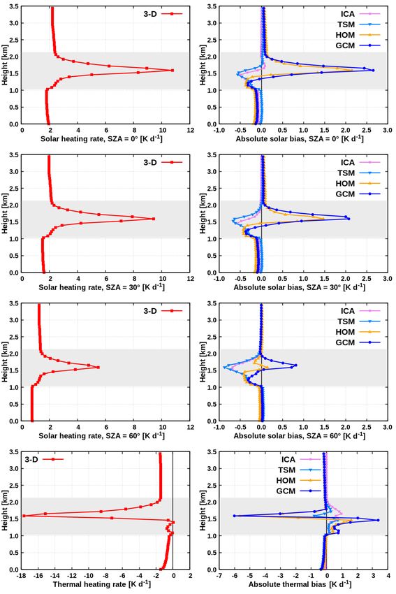
N. Črnivec and B. Mayer: The Tripleclouds method and its application to shallow cumulus clouds                                     10735

Figure 1. Divergent modeling of cloud–radiation interaction (arrows denote radiative fluxes; grey shading mirrors cloud optical thickness):
(b) realistic 3-D radiation calculation on a high-resolution cloud; (c) the ICA approximation; (d) the conventional plane-parallel approach
in coarse-resolution weather and climate models; (e) the McICA algorithm (rainbow-colored fluxes indicate calculations in various spectral
bands); (f) the Tripleclouds methodology.

per is to document the present Tripleclouds implementation              Tripleclouds radiation scheme. Shallow cumulus clouds are
in the comprehensive radiative transfer package libRadtran              convective clouds, which are often treated with the “core–
(Mayer and Kylling, 2005; Emde et al., 2016). Another aim               shell model” (Heus and Jonker, 2008; Heiblum et al., 2019).
of this study is to explore the TC potential for shallow cumu-          In this model, the convective cloud “core” associated with
lus clouds, applying various solver configurations diagnosing           updraft motion and increased condensate loading is located
atmospheric heating rate and net surface flux. The challenge            in the geometrical center of the cloud, surrounded by the
is to optimally set the condensate pair characterizing the two          cloud “shell” associated with downdrafts and condensate
cloudy regions and geometrically split the layer cloudiness.            evaporation. The core–shell model is supported by multiple
We test the validity of global FSD estimate in conjunction              observational studies (e.g., Heus et al., 2009; Rodts et al.,
with various assumptions for subgrid cloud condensate dis-              2003; Wang et al., 2009) and numerical modeling investiga-
tribution, which is of practical importance for the application         tions (e.g., Heus and Jonker, 2008; Jonker et al., 2008; Seigel,
in weather and climate models.                                          2014) and hence represents the essence of several convec-
   The paper is organized as follows: in Sect. 2, the cloud             tion parameterizations. Heiblum et al. (2019) showed that
data and methodology are introduced. In Sect. 3, our version            the core–shell model is valid for about 90 % of the typical
of the TC radiation scheme is presented. In Sect. 4, existing           cloud’s lifetime, with the largest discrepancy from the as-
approaches for generating cloud condensate pairs are revised.           sumed core–shell geometry occurring during the dissipation
TC performance is evaluated in Sect. 5. A brief summary and             stage of the cloud. Whereas most of the clouds contain a sin-
concluding remarks are given in Sect. 6.                                gle core, larger clouds can possess multiple cores. Similarly,
                                                                        clouds in a cloud field have multiple cores, whereby their
                                                                        aggregate effect can be modeled with a core–shell model
2     Cloud data and methodology                                        (Heiblum et al., 2019).

We first introduce the core–shell model for convective clouds
                                                                        2.1.2   Shallow cumulus cloud field case study
as well as the shallow cumulus case study in Sect. 2.1. The
radiative transfer models and experimental setup are outlined
in Sect. 2.2. The results of preliminary radiation experiments          Input for radiative transfer calculations is a shallow cumulus
demonstrating the importance of representing cloud horizon-             cloud field with a total cloud cover of 54.8 % (visualized in
tal heterogeneity are presented in Sect. 2.3.                           Fig. 2), simulated with the University of California, Los An-
                                                                        geles, large-eddy simulation (UCLA-LES) model (Stevens
2.1     Shallow cumulus clouds                                          et al., 2005; Stevens, 2007). The horizontal domain size is
                                                                        51.2 × 51.2 km2 , with the vertical extent of the domain be-
2.1.1    Core–shell model for convective clouds                         ing 3.5 km. A constant horizontal grid spacing of 100 m is
                                                                        applied, whereas the vertical grid spacing is variable rang-
A brief note regarding the horizontal distribution of cloud             ing from 50 m at the ground to 84 m at domain top. Further
condensate in convective cloud systems is provided herein.              details about the UCLA-LES setup can be found in Jakub
This knowledge will be exploited later when constructing the            and Mayer (2017). A 3-D LWC distribution was extracted

https://doi.org/10.5194/acp-20-10733-2020                                              Atmos. Chem. Phys., 20, 10733–10755, 2020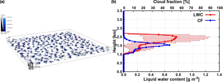
10736                   N. Črnivec and B. Mayer: The Tripleclouds method and its application to shallow cumulus clouds

Figure 2. (a) Shallow cumulus cloud field used as input for radiative transfer calculations (visualization with VisIt; Childs et al., 2012).
(b) Averaged LWC, its standard deviation (marked with error bars) and cloud fraction.

Figure 3. Horizontal heterogeneity for shallow cumulus cloud field. (a) Cloud mask (clouds in white; clear sky in black). (b) Vertically
integrated cloud optical thickness in the visible spectral range, highlighting solely optically thicker convective cores.

from a simulation snapshot (with a threshold of 10−3 g m−3 )            tracing of photons in cloudy atmospheres (Mayer, 2009),
and the corresponding effective radius (Re ) was parameter-             which can be run in ICA mode as well. Further, we employed
ized according to Bugliaro et al. (2011). Vertical profiles of          the classic δ-Eddington two-stream method (Zdunkowski et
averaged LWC, its standard deviation (σLWC ; simplest mea-              al., 2007) suitable for horizontally homogeneous layers (ei-
sure of cloud horizontal inhomogeneity) and cloud fraction              ther fully cloudy or fully clear sky) and the extension of this
are shown in Fig. 2b. Figure 3 shows the cloud mask as well             method, which allows for partial cloudiness. The latter is
as vertically integrated cloud optical thickness, demonstrat-           the δ-Eddington two-stream method with maximum-random
ing that optically thicker regions are located in the interior of       overlap assumption, which was recently implemented in li-
individual clouds, which conforms to the core–shell model.              bRadtran in the configuration as described in Črnivec and
                                                                        Mayer (2019) and is ideally suited as a proxy for the conven-
2.2     Radiative transfer models and experimental setup                tional GCM radiation scheme.

2.2.1    Radiative transfer models                                      2.2.2    Setup of radiative transfer experiments

The radiative transfer experiments were performed us-                   The background thermodynamic state was the US standard
ing the libRadtran software (http://www.libradtran.org,                 atmosphere (Anderson et al., 1986). The parameterization of
10 July 2020), which contains several radiation solvers. The            Hu and Stamnes (1993) was used to convert LWC and Re
benchmark calculations were performed with the 3-D model                into cloud optical properties. The solar experiments were per-
MYSTIC, the Monte Carlo code for the physically correct                 formed for solar zenith angles (SZAs) of 0, 30 and 60◦ and

Atmos. Chem. Phys., 20, 10733–10755, 2020                                                 https://doi.org/10.5194/acp-20-10733-2020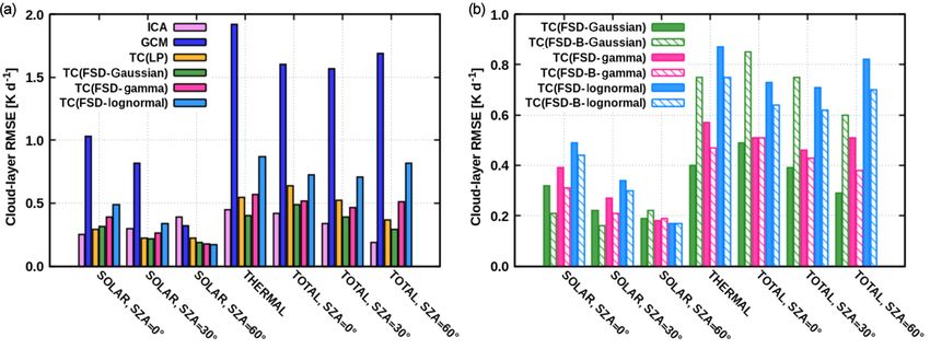
N. Črnivec and B. Mayer: The Tripleclouds method and its application to shallow cumulus clouds                                    10737

Table 1. List of preliminary radiative transfer experiments and their abbreviations.

                             Experiment                                                           Abbreviation
                             3-D Monte Carlo radiative model on LES cloud field                   3-D
                             ICA Monte Carlo radiative model on LES cloud field                   ICA
                             δ-Eddington two-stream method on LES cloud field                     TSM
                             δ-Eddington two-stream method on homogenized LES cloud field         HOM
                             δ-Eddington two-stream method with maximum-random overlap            GCM

a surface albedo of 0.25. In the thermal part of the spectrum,            interest is a single vertical profile of radiative heating rate;
the surface was assumed to be nonreflective. The shortwave                thus, results were horizontally averaged across the domain.
calculations applied 32 spectral bands of the correlated-k dis-           Figure 5 (left) shows the resulting benchmark profiles.
tribution by Kato et al. (1999), whereas the longwave cal-                   In the solar experiment for overhead Sun (Fig. 5, top left),
culations employed 12 spectral bands adopted from Fu and                  there is a large absorption of radiation in the cloud layer,
Liou (1992). In the Monte Carlo experiments, the standard                 resulting in a peak heating rate of 10.8 K d−1 . The latter
forward and the efficient backward photon tracing were em-                is reached at a height of 1.6 km, which is slightly above
ployed in the solar and thermal spectral range respectively.              the height of maximal cloud fraction (Fig. 2b). With de-
The resulting Monte Carlo noise of domain-averaged quanti-                creasing Sun elevation, the solar heating rate diminishes, ex-
ties is negligible (less than 0.1 %).                                     hibiting the maximum of 9.4 and 5.5 K d−1 at SZAs of 30
                                                                          and 60◦ , respectively. The height where the peak heating is
2.2.3    Diagnostics and error calculation                                reached stays the same at all SZAs. In the thermal spectral
                                                                          range (Fig. 5, bottom left), the cloud layer is subjected to
The radiative diagnostics include atmospheric heating rate                strong cooling, reaching a peak value of 17.7 K d−1 attained
and net (difference between downward and upward) surface                  at the same height as the maximum solar heating. Below this
flux. Each diagnostic was examined in the solar, thermal                  height, the magnitude of cooling decreases towards the cloud
(nighttime effect) and total (daytime effect) spectral range.             base, where a slight warming effect is observed.
The error is given by the absolute bias (Eq. 1), relative bias
(Eq. 2) and for the atmospheric heating rate additionally by              2.3.2   Conventional GCM representation
the root mean square error evaluated throughout the vertical
extent of the cloud layer (Eq. 3):                                        In order to mimic the conditions in conventional GCM mod-
                                                                          els (Fig. 4c), the cloud optical properties in each vertical
absolute bias = y − x,                                           (1)      layer were horizontally averaged over the cloudy part of the

                  y                                                       domain, creating a suite of plane-parallel partially cloudy
relative bias =     − 1 · 100 %,                                 (2)
                  x                                                       layers. Consequently, the δ-Eddington two-stream method
                      q                                                   with maximum-random overlap assumption was employed
cloud-layer RMSE = (y − x)2 ,                                    (3)      (abbreviated as the “GCM” experiment).
                                                                             The main shortcomings of the GCM compared to the
where y represents the biased quantity and x represents the
                                                                          benchmark (Fig. 5, right) are as follows. In the solar spec-
benchmark.
                                                                          tral range, the peak heating rate is overestimated by 2.7, 2.1
2.3     Preliminary radiative transfer experiments                        and 0.8 K d−1 at SZAs of 0, 30 and 60◦ , respectively. In the
                                                                          thermal spectral range, the GCM bias artificially enhances ra-
We present a set of preliminary radiative transfer experiments            diatively driven destabilization of the cloud layer by an over-
(listed in Table 1), introducing the 3-D benchmark, the ICA               estimation of cooling by 6.0 K d−1 at cloud-layer top and an
and the conventional GCM calculation. Further, we aim to                  overestimation of warming by 3.4 K d−1 at cloud-layer bot-
quantify the various error sources of GCM radiative heating               tom. The GCM error sources are multiple: the misrepresen-
rates, in particular the error related to neglected cloud hori-           tation of realistic cloud structure, the neglected subgrid hori-
zontal heterogeneity.                                                     zontal photon transport as well as the intrinsic difference be-
                                                                          tween the Monte Carlo and two-stream radiative solvers.
2.3.1    Benchmark heating rate
                                                                          2.3.3   ICA and its limitations
The benchmark calculation using MYSTIC (abbreviated as
the “3-D” experiment) was performed on the highly resolved                To quantify the effect of neglected horizontal photon trans-
LES cloud field (Fig. 4a). Supposing that the entire LES do-              port, we run the Monte Carlo radiative model in independent
main is contained within one GCM column, the quantity of                  column mode on the original cloud field preserving its LES

https://doi.org/10.5194/acp-20-10733-2020                                               Atmos. Chem. Phys., 20, 10733–10755, 2020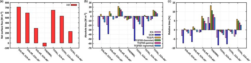
10738 N. Črnivec and B. Mayer: The Tripleclouds method and its application to shallow cumulus clouds
GCM error source is indeed the neglected cloud horizontal
heterogeneity. The question that we attempt to answer is how
much of this bias can be removed with Tripleclouds. In other
words, how well can the continuous probability density func-
tion (PDF) of layer LWC be represented by just two cloudy
regions (a two-point PDF)?
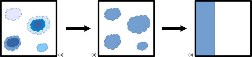
Figure 4. (a) A horizontal cross section of LES cloud field. (b)
Derived “homogenized” cloud field, which retains its 3-D geome-
try but where horizontal heterogeneity is completely removed by 3 The Tripleclouds radiative solver
applying averaged cloud optical properties in each vertical layer.
(c) Conditions in a grid box of a conventional GCM (homogeneous The underlying δ-Eddington two-stream framework em-
fractional cloudiness). ployed in the present Tripleclouds implementation differs
from that applied by SH08 and subsequent studies (e.g.,
Shonk et al., 2010; Hogan et al., 2019), whereby the latter
resolution (Fig. 4a), with the result horizontally averaged is based on the adding method (Lacis and Hansen, 1974)
over the domain (abbreviated as the “ICA” experiment). Sim- as originally included in the Edwards and Slingo (1996) ra-
ilarly, we applied the δ-Eddington two-stream method within diation scheme. Therefore, we first present the δ-Eddington
each independent column of the original LES grid (Fig. 4a) two-stream method (Zdunkowski et al., 2007), already previ-
and subsequently averaged the result horizontally (abbrevi- ously contained in libRadtran, and introduce the terminology
ated as the “TSM” experiment). The difference between the in Sect. 3.1. We focus only on those aspects of the method,
ICA and 3-D is a measure of horizontal photon transport. The important to understand its extension to multiple (three) re-
difference between the TSM and 3-D is a measure of both the gions, explained in subsequent Sect. 3.2. The novel over-
horizontal photon transport as well as the intrinsic difference lap formulation based on the core–shell model is established
between the Monte Carlo and two-stream radiative solvers. in Sect. 3.3. Further technical instructions regarding Triple-
As anticipated, both independent column experiments clouds usage within the scope of libRadtran are provided in
(ICA, TSM) perform similarly (Fig. 5, right), implying that Appendix A.
the intrinsic difference between the radiative solvers is small.
Therefore, only the ICA is discussed hereafter. The solar 3.1 δ-Eddington two-stream method
bias increases with descending Sun (cloud side illumination;
Hogan and Shonk, 2013; Jakub and Mayer, 2015, 2016), In the classic two-stream approach, the entire radiative field
reaching a maximum of −0.7 K d−1 at an SZA of 60◦ . The is approximated solely with direct solar beam (S) and two
amount of thermal cooling is underestimated in the ICA (up streams of diffuse radiation: the downward (E↓ ) and upward
to 1 K d−1 ), since realistic cloud side cooling is neglected (E↑ ) component. The widely employed δ-Eddington approx-
(Kablick et al., 2011; Klinger and Mayer, 2014, 2016). Nev- imation is a reliable way to account for a strong forward-
ertheless, the ICA still overall performs considerably better scattering peak of cloud droplets (Joseph et al., 1976; King
than the conventional GCM, implying that the major error and Harshvardhan, 1986; Stephens et al., 2001). For the cal-
source of GCM heating rate stems from the misrepresenta- culations in a vertically inhomogeneous atmosphere, the at-
tion of cloud structure and not from the neglected horizontal mosphere is divided into a number of homogeneous layers,
photon transport. each characterized by its set of constant optical properties.
Considering a single layer (j ) located between levels (i − 1)
2.3.4 Cloud horizontal heterogeneity effect and (i) (illustrated in Fig. 6)1 , a system of linear equations
determining the fluxes emanating from the layer as a func-
In order to isolate the effects of neglected cloud horizontal tion of fluxes entering the layer can be written as
heterogeneity in a conventional GCM from other effects re-
lated to the misrepresentation of cloud structure (e.g., vertical E↑ (i − 1) a11 a12 a13 E↑ (i)
overlap assumption), we employed the GCM radiative solver E↓ (i) = a12 a11 a23 · E↓ (i − 1) . (4)
on the cloud field preserving its LES resolution but with re- S(i) 0 0 a33 S(i − 1)
moved horizontal heterogeneity (Fig. 4b). In this way, the av-
eraged (plane-parallel) cloud optical properties were applied The coefficients akl in Eq. (4) are referred to as Eddington
in each vertical layer, but the realistic 3-D cloud field ge- coefficients. They depend on the optical properties of layer
ometry was retained. The results were horizontally averaged (j ) and have the following physical meaning:
(abbreviated as the “HOM” experiment). 1 We follow the convention of i, j increasing downward from the
The radiative heating rate in the HOM experiment (Fig. 5, top of the atmosphere, where i = 0, j = 1. Index i is used for level
right) is to a great extent similar to that in the GCM (espe- variables, while index j is used for layer variables. The N vertical
cially in the solar experiments at SZAs of 0 and 30◦ , as well layers, enumerated from 1 to N , are enclosed by (N + 1) vertical
as in the thermal experiment), implying that the dominant levels, enumerated from 0 to N.
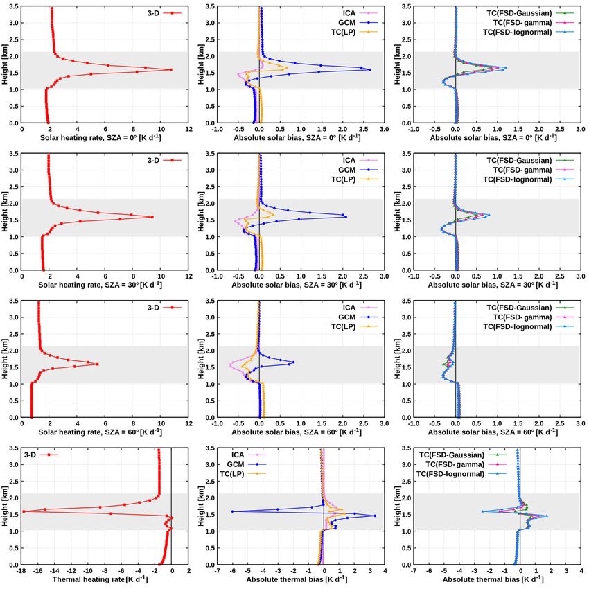
Atmos. Chem. Phys., 20, 10733–10755, 2020 https://doi.org/10.5194/acp-20-10733-2020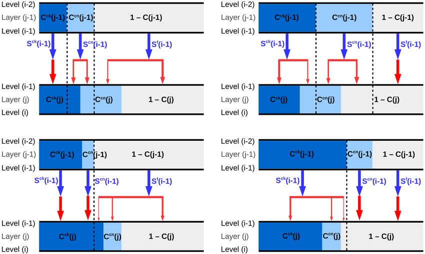
N. Črnivec and B. Mayer: The Tripleclouds method and its application to shallow cumulus clouds                            10739

Figure 5. Radiative heating rate in preliminary experiments. The cloud layer is shaded grey.

https://doi.org/10.5194/acp-20-10733-2020                                               Atmos. Chem. Phys., 20, 10733–10755, 2020
10740 N. Črnivec and B. Mayer: The Tripleclouds method and its application to shallow cumulus clouds
– a11 – transmission coefficient for diffuse radiation,
– a12 – reflection coefficient for diffuse radiation,
– a13 – reflection coefficient for the primary scattered so-
lar radiation,
– a23 – transmission coefficient for the primary scattered
solar radiation and
– a33 – transmission coefficient for the direct solar radia-
Figure 6. A homogeneous model layer between levels (i − 1) and
tion. (i). Incoming radiative fluxes are colored red; outgoing fluxes are
colored blue.
The preceding formulation considered solar radiative
transfer in the absence of thermal emission. As solar and ther-
mal spectra are separated and can be therefore conveniently both cloudy and the cloud-free components:
treated independently, the solar source is merely replaced
with the terrestrial emission term when addressing thermal S(i) = S ck (i) + S cn (i) + S f (i), (7)
radiation. The vertical temperature variation is thereby taken E↓ (i) = E↓ck (i) + E↓cn (i) + E↓f (i), (8)
into account by allowing the Planck function to vary in ac-
cordance with the Eddington-type linearization: BPlanck (τ ) = E↑ (i) = E↑ck (i) + E↑cn (i) + E↑f (i). (9)
B0 + B1 τ , where B0 and B1 are constants. The equation sys-
Equation (4) is replaced by
tem for a single layer is constructed in a similar manner,
accounting for both upward and downward thermal emis-
sion contributions. For a more comprehensive explanation, ck
E↑ (i − 1)
ck
a11 a12 ck a ck
13
the reader is referred to Zdunkowski et al. (2007), as in the E ck (i) = a ck a ck a ck
↓ 12 11 23
rest of this section we will focus on solar radiation. ck
S ck (i) 0 0 a33
The individual layers are coupled vertically by imposing
T↑ck, ck E↑ck (i) + T↑cn, ck E↑cn (i) + T↑f, ck E↑f (i)
flux continuity at each level. Taking the boundary conditions
at TOA (Eq. 5) and at the ground (Eq. 6, with Ag representing · T↓ck, ck E↓ck (i − 1) + T↓cn, ck E↓cn (i − 1) + T↓f, ck E↓f (i − 1) ,
ground albedo) into account: T↓ck, ck S ck (i − 1) + T↓cn, ck S cn (i − 1) + T↓f, ck S f (i − 1)
(10)
E↓ (0) = 0, (5) cn cn cn cn
E↑ (N ) = Ag [S(N ) + E↓ (N )], (6) E↑ (i − 1) a11 a12 a13
E cn (i) = a cn a cn a cn
↓ 12 11 23
cn
the radiative fluxes throughout the atmosphere are computed S cn (i) 0 0 a33
by solving the matrix problem (Coakley and Chylek, 1975;
T↑ck, cn E↑ck (i) + T↑cn, cn E↑cn (i) + T↑f, cn E↑f (i)
Wiscombe and Grams, 1976; Meador and Weaver, 1980; Rit-
· T↓ck, cn E↓ck (i − 1) + T↓cn, cn E↓cn (i − 1) + T↓f, cn E↓f (i − 1) ,
ter and Geleyn, 1992). Henceforth, the calculation of heating
rates is straightforward. T↓ck, cn S ck (i − 1) + T↓cn, cn S cn (i − 1) + T↓f, cn S f (i − 1)
(11)
3.2 δ-Eddington two-stream method for three regions f
E↑ (i − 1)
f f f
a11 a12 a13
at each height E f (i) = a f f f
↓ 12 a11 a23
f 0 0 a33 f
Consider now a model layer located between levels (i − 1) S (i)
and (i) divided into three regions (Fig. 7). Such layer is char- T↑ck, f E↑ck (i) + T↑cn, f E↑cn (i) + T↑f, f E↑f (i)
acterized by three sets of optical properties and correspond-
· T↓ck, f E↓ck (i − 1) + T↓cn, f E↓cn (i − 1) + T↓f, f E↓f (i − 1) ,
ing Eddington coefficients: one for the region of optically
thick cloud (superscript “ck”), the other for the region of T↓ck, f S ck (i − 1) + T↓cn, f S cn (i − 1) + T↓f, f S f (i − 1)
optically thin cloud (superscript “cn”) and the third for the (12)
cloud-free region (superscript “f”). In order to apply vertical
overlap rules, the radiative fluxes corresponding to each of so that the fluxes emanating from a certain region of
the three regions need to be defined separately at each level the layer under consideration (e.g., region of optically thick
(e.g., S ck , S cn and S f ; and analogously for both diffuse com- cloud) generally depend on a linear combination of the in-
ponents). Total radiative flux at level (i) is thus the sum of coming fluxes stemming from each of the three regions in
Atmos. Chem. Phys., 20, 10733–10755, 2020 https://doi.org/10.5194/acp-20-10733-2020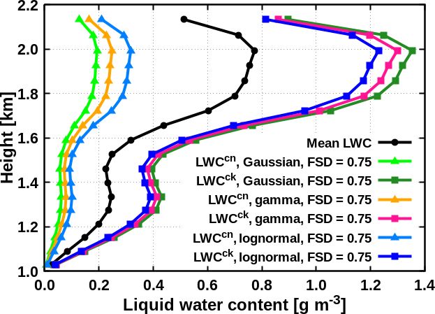
N. Črnivec and B. Mayer: The Tripleclouds method and its application to shallow cumulus clouds                                     10741

                                                                      Therefore, we additionally assume the maximum overlap of
                                                                      optically thicker cloudy regions in pairs of adjacent layers
                                                                      and abbreviate this extended overlap rule to the “maximum2 -
                                                                      random overlap”. This assumption implicitly places the opti-
                                                                      cally thicker cloudy region towards the interior of the cloud
Figure 7. A model layer between levels (i − 1) and (i) divided into   in the horizontal plane, which is in line with the core–shell
three regions.                                                        model.
                                                                         Now one can quantitatively determine the overlap coeffi-
                                                                      cients in Eqs. (10), (11) and (12) for the maximum2 -random
adjacent layers. The coefficients starting with T appearing
                                                                      overlap. We consider the transmission of downward radia-
in Eqs. (10), (11), (12) are referred to as the overlap (trans-
                                                                      tion through two adjacent layers with partial cloudiness. Four
fer) coefficients and correspond to layer (j ). The coefficient
                                                                      possible geometries, illustrated in Fig. 8, need to be treated.
T↓ck, cn (j ), for example, represents the fraction of downward
                                                                      For the situation depicted in the top left panel of Fig. 8, the
radiation that leaves the base of optically thick cloud of layer
                                                                      transmission of direct radiation can be formulated as follows.
(j −1) and enters the optically thin cloud of layer under con-
                                                                      The optically thick cloud of layer (j −1) transmits S ck (i −1),
sideration (j ). The overlap coefficients quantitatively depend
                                                                      the optically thin cloud transmits S cn (i − 1) and the cloud-
on the choice of the overlap rule, which will be discussed in
                                                                      free region transmits S f (i − 1). These three components of
the next section. For a three-region layer, the boundary con-
                                                                      the transmitted radiation must then be distributed between
dition at TOA (Eq. 5) implies
                                                                      the three regions of the lower layer (j ). The maximum over-
                                                                      lap of optically thick cloudy regions implies that the entire
E↓ck (0) = 0,                                                 (13)
                                                                      radiation S ck leaving the base of layer (j − 1) enters the op-
E↓cn (0) = 0,                                                 (14)    tically thick cloud below:
E↓f (0) = 0.                                                  (15)
                                                                      T↓ck, ck (j ) = 1,                                             (22)
The boundary condition at the ground (Eq. 6) is extended to
                                                                      and none of it enters the other two regions:
E↑ck (N ) = Ag [S ck (N ) + E↓ck (N )],                       (16)
                                                                      T↓ck, cn (j ) = 0,                                             (23)
E↑cn (N ) = Ag [S cn (N ) + E↓cn (N )],                       (17)
                                                                      T↓ck, f (j ) = 0.                                              (24)
E↑f (N ) = Ag [S f (N ) + E↓f (N )],                          (18)
                                                                      To ensure the maximum overlap of cloudy layers as a whole,
which assumes that the downward fluxes leaving the low-               the remaining cloudy flux at the base of layer (j −1), namely
est model layer, after reflection enter the same sections of          the S cn (i − 1), needs to be led into the two cloudy regions of
individual cloudy and cloud-free air (isotropic ground reflec-        the lower layer, with the priority to enter the optically thick
tion).                                                                cloud. This yields
3.3    Overlap considerations                                                         C ck (j ) − C ck (j − 1)
                                                                      T↓cn, ck (j ) =                          ,                     (25)
                                                                                            C cn (j − 1)
The layer cloud fraction C is given by
                                                                                      [C ck (j − 1) − C cn (j − 1)] − C ck (j )
                                                                      T↓cn, cn (j ) =                                           ,    (26)
C(j ) = C ck (j ) + C cn (j ).                                (19)                                   C cn (j − 1)

In our implementation, we demand the following relationship           T↓cn, f (j ) = 0.                                              (27)
between the individual cloud fraction components:
                                                                      The cloud-free flux S f at the base of layer (j − 1) is dis-
  ck                                                                  tributed according to
C (j ) = α · C(j ),                                           (20)
  cn
C (j ) = (1 − α) · C(j ),                                     (21)                    1 − C(j )
                                                                      T↓f, f (j ) =              ,                                   (28)
where α is a constant between 0 and 1. We apply the widely                          1 − C(j − 1)
                                                                                     C(j ) − C(j − 1)
used maximum-random overlap assumption (Geleyn and                    T↓f, cn (j ) =                  ,                              (29)
Hollingsworth, 1979) for the entire layer cloudiness (sum                              1 − C(j − 1)
of optically thick and thin cloudy regions), where adjacent           T↓f, ck (j ) = 0.                                              (30)
cloudy layers exhibit maximal overlap and cloudy layers sep-
arated by at least one cloud-free layer exhibit random over-          The derivation of overlap coefficients for other three geome-
lap. If the cloudy layers are split into two parts, however,          tries involves analogous considerations, whereby the result-
this overlap rule is not sufficient and needs to be extended.         ing formulas as well as their generalized formulation are

https://doi.org/10.5194/acp-20-10733-2020                                                 Atmos. Chem. Phys., 20, 10733–10755, 2020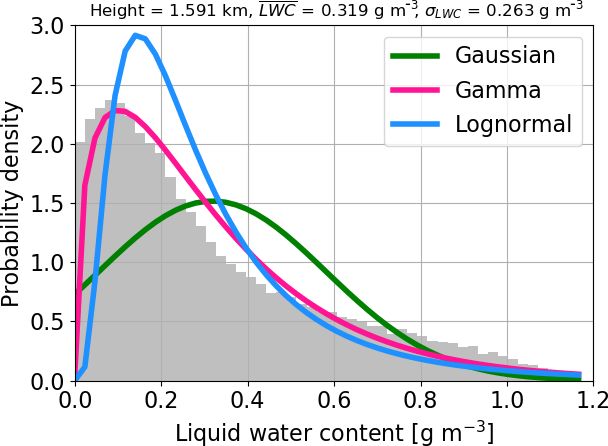
10742                  N. Črnivec and B. Mayer: The Tripleclouds method and its application to shallow cumulus clouds

Figure 8. Transmission of direct solar radiation through two adjacent layers with partial cloudiness for the maximum2 -random overlap
concept.

given in Appendix B. The transmission of upward radiation            method” (Shonk et al., 2010), which can only be applied if
is managed via overlap coefficients T↑a, b (j ) in an equivalent     the LWC distribution is known. In Sect. 4.2, we summarize
manner, except that these are dependent on the cloud frac-           the more practical “fractional standard deviation method”
tion in the layer under consideration and that in the layer un-      (Shonk et al., 2010).
derneath [C(j ), C(j + 1)]. It should be noted that the same
coefficients govern the reflection, whereby the upward reflec-       4.1   The lower percentile method
tion of downward radiation is treated with T↓a, b and the re-
                                                                     In this method, it is assumed that the LWC distribution in
verse situation is treated with T↑a, b . Pairwise overlap as em-     each vertical layer can be approximated with the normal dis-
ployed here ensures that the matrix problem is fast to solve.        tribution:
Whereas a drawback of the core–shell model and thereby the
                                                                                                     (LWC − LWC)2

outlined overlap is that it underperforms in the case of ver-                          1
                                                                     p(LWC) = √              exp −          2
                                                                                                                       ,    (31)
tically developed cloud systems in strongly sheared condi-                          2π σLWC              2σLWC
tions, the present Tripleclouds implementation is an excellent
tool to study shallow convective clouds. In this way, the ef-        where LWC is layer mean LWC and σLWC is its standard
fects of cloud horizontal inhomogeneity are tackled in isola-        deviation. The distribution of LWC is divided into two re-
tion, while the issues related to vertical shear are eliminated.     gions through a given percentile of the distribution, denoted
   The Tripleclouds radiative solver has been successfully           as “split percentile (SP)”. The latter is chosen to be the 50th
implemented in the libRadtran package. Technically, the              percentile or the median, which splits the cloud volume into
calculation of overlap coefficients is performed in an au-           two equal parts (i.e., cloud fraction in each vertical layer is
tonomous function enabling flexible modifications of overlap         halved). The LWC of the optically thin cloud (LWCcn ) is de-
rules in the future.                                                 termined as the value corresponding to the so-called “lower
                                                                     percentile (LP)” of the distribution. This is chosen to be the
                                                                     16th percentile based on the following considerations. We
                                                                     adjust the two LWC values in a way that the mean LWC in
4   Methodologies to generate the LWC pair
                                                                     the layer is conserved:
In order to apply the TC radiative solver, a pair of LWC char-                LWCck + LWCcn
acterizing optically thin and thick cloudy regions (LWCcn ,          LWC =                      ,                               (32)
                                                                                      2
LWCck ) needs to be created in each vertical layer. In
                                                                     and that they are separated by 2 standard deviations:
Sect. 4.1, we revise the original Tripleclouds method intro-
duced by SH08, later referred to as the “lower percentile            LWCck − LWCcn = 2σLWC .                                    (33)

Atmos. Chem. Phys., 20, 10733–10755, 2020                                            https://doi.org/10.5194/acp-20-10733-2020
N. Črnivec and B. Mayer: The Tripleclouds method and its application to shallow cumulus clouds 10743
Figure 9. LWC profiles obtained with the LP method.
Figure 10. The actual FSD of the shallow cumulus. The grey-
shaded area represents the uncertainty of global FSD estimate, cen-
For a Gaussian distribution, the latter constraint has a desired tered around its mean value (black line).
property that the variability within each of the two cloudy
regions (measured by σLWC ) is the same as that within the
entire cloud in the layer. Equations (32) and (33) give the
following relationship for LWCcn :
LWCcn = LWC − σLWC . (34)
The fraction of the distribution with LWC lower than LWCcn
is therefore
Z cn
LWC
fcn = p(LWC)dLWC = 0.159, (35)
−∞
which corresponds to the LP of 16. Finally, the LWCck is
determined using Eq. (32) to conserve the mean. Figure 9
shows the resulting LWC pair when the LP method is applied
on shallow cumulus cloud field. Figure 11. LWC profiles obtained with the FSD method using mean
It should be noted that the choice of the 16th percentile global estimate and altering LWC distribution.
as the LP and the 50th percentile as the SP is based solely
on theoretical considerations. In practice, the LP and SP are
the two tunable parameters, that can be adjusted according to
Since in practice only LWC is known within a GCM grid
their performance on real cloud data. Even though the opti-
box, the FSD has to be parameterized. A review of numer-
mal setting varies, SH08 exposed that the combination of LP
ous studies (Cahalan et al., 1994a; Barker et al., 1996; Pin-
of 16 and SP of 50 generally serves well in both solar and
cus et al., 1999; Smith and Del Genio, 2001; Rossow et al.,
thermal spectral range for vast ranges of cloud data.
2002; Hogan and Illingworth, 2003; Oreopoulos and Caha-
4.2 Fractional standard deviation method lan, 2005; SH08) carried out by Shonk et al. (2010) gave a
globally representative FSD of 0.75 ± 0.18. Figure 10 shows
This method in its initial formulation by Shonk et al. (2010) the actual FSD for the present shallow cumulus: although this
implicitly assumes that LWC is normally distributed as well. FSD is strongly dependent on the position within the cloud
Thereby the cloudiness in each vertical layer is partitioned layer, it predominantly lies within the range of global esti-
into two regions of equal size and the pair of LWC (LWCcn , mate.
LWCck ) is obtained by If the cloud condensate is normally distributed, subtracting
σLWC from the LWC to obtain the LWCcn in Eq. (36) cor-
LWCck, cn = LWC ± σLWC = LWC(1 ± FSD), (36) responds approximately with the 16th percentile. For more
where FSD represents the fractional standard deviation of realistic lognormal and gamma distributions, the 16th per-
LWC: centile (advocated by SH08) is given by relationships pre-
σLWC sented in Hogan et al. (2016, 2019), whereby the LWCck is
FSD = . (37) again obtained by conserving the layer mean.
LWC
https://doi.org/10.5194/acp-20-10733-2020 Atmos. Chem. Phys., 20, 10733–10755, 202010744 N. Črnivec and B. Mayer: The Tripleclouds method and its application to shallow cumulus clouds
In order to test the validity of global FSD estimate, we layer reduced by a factor of 5. At an SZA of 60◦ , the maximal
applied its mean value (0.75) to create the pair of LWC in bias of 0.8 K d−1 within the cloud layer becomes of the oppo-
each vertical layer containing cloud. Further, to test the sen- site sign but is still smaller in magnitude (−0.4 K d−1 ), when
sitivity of TC radiative quantities to the assumed form of the the TC(LP) is applied in place of the conventional GCM. In
subgrid cloud condensate distribution, we employed the FSD the layer above and especially below the cloud layer, how-
method in conjunction with all three distribution assumptions ever, the bias is slightly increased. Finally, it should be noted
(Gaussian, gamma, lognormal). The resulting LWC profiles that at low Sun (SZAs of 30 and 60◦ ) the TC is generally even
are shown in Fig. 11, demonstrating that the LWC pair char- more accurate than the ICA, which could be partially due to
acterizing the two cloudy regions is clearly sensitive to the effective treatment of solar 3-D effects in the TC scheme. It
distribution assumption, when the mean global FSD estimate is noteworthy that, at all three SZAs, the 3-D radiation fea-
is used as a proxy for cloud horizontal inhomogeneity degree. ture at cloud base (increased heating due to surface reflection
of radiation) cannot be properly accounted for using the TC
solver.
5 Application In the thermal spectral range (Fig. 12, bottom middle), the
degree of artificially enhanced destabilization of the cloud
We evaluated the TC radiative solver with both LP and FSD
layer, arising from the overestimation of cloud-top cooling
methods. The effective radii characterizing the two cloudy
and cloud base warming in the GCM, is drastically reduced
regions were kept the same (averaged Re ). The setup of radi-
when the TC(LP) is applied, interpreted as follows. The non-
ation calculations was as described in Sect. 2.2. The results
homogeneous clouds have lower mean longwave emissiv-
of the various TC experiments are compared with the con-
ity and absorptivity than the corresponding homogeneous
ventional GCM, which approximates the cloud condensate
clouds with the same mean optical depth. Thus, the non-
distribution with a one-point PDF and can be perceived as an
homogeneous cloud top in the TC experiment emits less ra-
upper bound for the tolerable TC error. In addition, the ICA,
diation compared to the homogeneous cloud top in the GCM
which resolves the full subgrid PDF, is shown as well. The
configuration, which reduces the negative GCM bias at cloud
atmospheric heating rate is discussed in Sect. 5.1, whereas
top. Similarly, the non-homogeneous cloud base in the TC
the net surface flux is investigated in Sect. 5.2.
experiment absorbs less of the radiation stemming from the
5.1 Atmospheric heating rate warmer atmospheric layers underneath the cloud, compared
to the homogeneous cloud base in the conventional GCM,
5.1.1 Tripleclouds with LP method which reduces the positive GCM bias at cloud base. As an-
ticipated, in the region above and below the cloud layer, the
We assess first the TC radiative solver when the LP method difference between the TC and the GCM is only marginal. It
is used to obtain the pair of LWC. The results of this exper- is noteworthy that the TC performs similarly well to the ICA
iment, denoted as “TC(LP)”, are shown in Fig. 12 (middle) also in the thermal spectral range, implying that the realistic
and Fig. 13a. It is apparent that the TC(LP) is overall sig- subgrid cloud variability can be adequately represented by a
nificantly more accurate than the GCM. In the solar spec- two-point PDF.
tral range for overhead Sun (Fig. 12, top middle), the maxi-
mal bias within the cloud layer is reduced from 2.7 to only 5.1.2 Tripleclouds with FSD method
0.7 K d−1 . Whereas the largest bias reduction is observed
within the cloud layer, the heating rate above and below We investigate now the TC experiments applying the FSD
the cloud layer is considerably improved as well, explained method together with global FSD estimate, shown in Fig. 12
as follows. The non-homogeneous clouds have lower mean (right) and Fig. 13a. The TC(FSD) experiment assuming the
shortwave albedo and absorptivity than the corresponding Gaussianity of cloud condensate is examined first – this ex-
plane-parallel cloudiness with the same mean optical depth periment is considerably more accurate than the conventional
(Fig. 2 of Cairns et al., 2000). This implies that the non- GCM as well. As an illustration, the daytime cloud-layer
homogeneous cloud in the TC configuration reflects less of RMSE of 1.7 K d−1 is reduced to 0.3 K d−1 at an SZA of 60◦
the incoming solar radiation upward (leading to a reduction (Fig. 13a). Furthermore, this TC(FSD) experiment is even
of the positive GCM bias above the cloud layer) and simulta- slightly more accurate than the TC(LP) especially in the ther-
neously absorbs less radiation (leading to a reduction of the mal spectral range and in the solar spectral range at SZAs of
positive GCM bias in the cloud layer), compared to the ho- 30 and 60◦ , whereas at an SZA of 0◦ the situation is reversed
mogeneous cloud in the GCM. Consequently, more radiation (Fig. 12). The largest discrepancy between the two TC exper-
is transmitted through the cloud layer and absorbed in the re- iments is observed in the central part of the cloud layer and
gion below the cloud layer in the TC experiment compared is attributed to the fact that the actual layer LWC distribution
to that in the GCM, which reduces the negative GCM bias in of the present shallow cumulus deviates from the assumed
this region. At an SZA of 30◦ , the behavior is qualitatively Gaussian distribution as well as that the actual FSD deviates
similar, with the maximal bias of 2.1 K d−1 within the cloud from the assumed global estimate.
Atmos. Chem. Phys., 20, 10733–10755, 2020 https://doi.org/10.5194/acp-20-10733-2020N. Črnivec and B. Mayer: The Tripleclouds method and its application to shallow cumulus clouds 10745 Figure 12. Left: benchmark radiative heating rate. Middle and right: bias for the ICA, GCM and TC experiments. In order to further support these findings, theoretical distri- gamma distributional fit performed best throughout the cen- butions (see also Appendix C) were fitted to the actual LWC tral part of the cloud layer, where cloud–radiative effect is distribution in each vertical cloudy layer (as illustrated in maximized. Fig. 14) and the Kolmogorov–Smirnov test (Conover, 1971; When examining the entire set of TC(FSD) experiments Wilks, 1995) was used to assess the goodness of fit. It was with global FSD, it is apparent that the radiative heating rate found that the actual LWC distribution is best approximated is considerably more accurate compared to the conventional with the gamma distribution (best fit in 55 % of the cloudy GCM regardless of the exact assumption for the LWC distri- layers), followed by the lognormal distribution, whereas the bution. Although the Gaussian distribution was ranked worst Gaussian distribution always ranked worst. Precisely, the when fitted to the actual PDF, the Gaussianity assumption https://doi.org/10.5194/acp-20-10733-2020 Atmos. Chem. Phys., 20, 10733–10755, 2020
10746                   N. Črnivec and B. Mayer: The Tripleclouds method and its application to shallow cumulus clouds

Figure 13. (a) RMSE for the ICA, GCM and TC experiments. (b) Comparison of the TC experiments using the FSD method in the baseline
setup with global estimate and with the parameterization of Boutle et al. (2014) (denoted as “B”). Note the different scales on the y axis.

                                                                        et al. (2014), the TC experiment with global FSD constant
                                                                        assuming Gaussian distribution remains the most accurate
                                                                        during both nighttime and daytime (Fig. 13b). To that end,
                                                                        the development of improved parameterizations is highly de-
                                                                        sired in the future.

                                                                        5.2   Net surface flux

                                                                        Shallow cumulus clouds are a vital part of the planetary
                                                                        boundary layer, where the atmosphere is directly influenced
                                                                        by the presence of the Earth’s surface. The net surface ra-
                                                                        diative flux is the key component of surface energy budget.
                                                                        The radiative biases at the surface, stemming from the inac-
                                                                        curate treatment of clouds, need to be properly understood
Figure 14. Actual LWC probability density in the central part of the    and possibly best eliminated, as they generally feed back on
cloud layer and distributional fits.                                    the biases in the cloudy layers, when the radiation scheme is
                                                                        coupled to a dynamical model.
                                                                           The behavior of surface biases underneath the present
with global FSD performed best in practice, contemplated as             shallow cumulus (Fig. 15b, c) is partially consistent with the
follows. In the central part of the cloud layer around max-             findings gained when examining the cloud-layer heating rate
imum cloud fraction, the actual FSD of the present shal-                error. In the ICA, the daytime net surface flux is underesti-
low cumulus (0.95) is larger than the assumed global esti-              mated compared to 3-D at all SZAs. This is primarily due
mate. The latter is primarily due to great amount of cloud              to well-acknowledged cloud side escape effect (Várnai and
side area in this region, an essential characteristic of broken         Davies, 1999; Hogan and Shonk, 2013), where the realistic
cloud field, which generally contributes to increased variabil-         scattering of radiation through cloud side areas increases 3-D
ity (Boutle et al., 2014; Hill et al., 2012, 2015). Since the           downward surface radiation. Even when the Sun is lower in
assumption of Gaussianity implies the largest difference be-            the sky (SZA of 60◦ ), this mechanism overcomes the oppos-
tween the LWC pair characterizing the two cloudy regions                ing cloud side illumination effect, where an elongated sur-
(Fig. 11), it partially accounts for the missing variability pro-       face shadow reduces the 3-D net surface flux. Similarly, the
vided by the global estimate.                                           strength of nocturnal surface cooling is overestimated in the
   Based upon these considerations, we additionally evalu-              ICA, since realistic cloud side emission is neglected.
ated the parameterization of Boutle et al. (2014) for liquid               The daytime GCM net flux bias at comparatively high
cloud inhomogeneity, which takes into account that vari-                Sun (SZAs of 0 and 30◦ ) is by a factor of 2 larger than the
ability is cloud fraction dependent. Although solar RMSE                ICA bias. This is attributed to the fact that the plane-parallel
slightly reduces when FSD is represented following Boutle               GCM cloudiness leads to an increased solar absorption and

Atmos. Chem. Phys., 20, 10733–10755, 2020                                                https://doi.org/10.5194/acp-20-10733-2020
N. Črnivec and B. Mayer: The Tripleclouds method and its application to shallow cumulus clouds 10747
Figure 15. (a) benchmark net surface radiative flux. (b, c) bias for the ICA, GCM and TC experiments.
hence reduced cloud-layer transmittance. The latter reduces The constructed Tripleclouds radiative solver was evalu-
downward flux reaching the surface and profoundly under- ated on a shallow cumulus cloud field. The validity of global
estimates the net flux. During nighttime, the plane-parallel estimate of fractional standard deviation (a common measure
cloud in the GCM emits a greater amount of radiation to- of cloud horizontal variability) as well as of more sophisti-
wards the surface compared to heterogeneous cloud in the cated inhomogeneity parameterization was tested along with
ICA, leading to a reduction of surface net flux bias. different assumptions for subgrid cloud condensate distri-
When Tripleclouds is applied – either with the LP or the bution (Gaussian, gamma, lognormal), which are frequently
FSD method utilizing the global estimate – instead of con- applied when representing clouds in weather and climate
ventional GCM radiation scheme, the daytime net surface models. In the vast majority of experiments, Tripleclouds
flux bias of −55 W m−2 (or −8 %) is substantially reduced performed better than the conventional plane-parallel GCM
to −5 W m−2 (or −1 %) at overhead Sun and similarly for scheme. The error of atmospheric heating rate was substan-
an SZA of 30◦ (assuming Gaussianity of cloud condensate). tially reduced during daytime and nighttime (up to a 5-
At an SZA of 60◦ and especially during nighttime, radiative fold cloud-layer RMSE reduction). In the event of net sur-
bias in the various TC experiments increases compared to face flux, the daytime bias was generally depleted as well,
the GCM bias. Similar findings are obtained if the FSD is whereas the nighttime bias was slightly enlarged, suggesting
parameterized according to Boutle et al. (2014), which does that the computationally more efficient plane-parallel scheme
not bring desired improvements (not shown). This indicates could be retained in this case.
that the TC in its current configuration should be taken with The question that needs to be addressed next is the ex-
caution when applied to surface thermal flux, as its usage can tent to which our findings for a shallow cumulus case study
lead to degradation of the nocturnal surface budget compared with intermediate cloud cover apply to a larger set of scenar-
to simple plane-parallel model. ios comprising a wide range of cloud cover. This question is
relevant because horizontal variability might essentially de-
pend on cloud fraction (Boutle et al., 2014; Hill et al., 2012,
6 Summary and conclusions 2015). Similarly, the degree of cloud horizontal variability
depends on the GCM grid resolution (Boutle et al., 2014;
Inspired by the Tripleclouds concept of Shonk and Hogan Hill et al., 2012, 2015), which has to be investigated in more
(2008), we incorporated a second cloudy region in the widely detail in the future. Furthermore, organizational aspects of
used δ-Eddington two-stream method with maximum- shallow convection should be addressed in the context of the
random overlap assumption for partial cloudiness. The re- present study. Mesoscale shallow convection sometimes oc-
sulting radiation scheme thus has one cloud-free and two curs in the form of uniformly scattered cumuli but is also
cloudy regions in each vertical layer and is capable of rep- frequently organized into cloud streets, clusters or mesoscale
resenting cloud horizontal variability. The inclusion of a sec- arcs (Agee et al., 1973; Atkinson and Zhang, 1996; Wood
ond cloudy region into the two-stream framework required and Hartmann, 2006; Seifert and Heus, 2013). The classifi-
an extension of vertical overlap rules. While retaining the cation of rich spatial patterns into various mesoscale cloud
maximum-random overlap for the entire layer cloudiness, morphologies can thereby valuably be performed with deep
we additionally assumed the maximum overlap of optically learning algorithms (e.g., Yuan et al., 2020). The robustness
thicker cloudy regions in pairs of adjacent layers. This im- of the present results on the nature of cloud organization
plicitly places the optically thicker region towards the inte- should be examined next. Recently, Stevens et al. (2019) pro-
rior of the cloud in the horizontal plane, while the optically posed four mesoscale cloud patterns frequently observed in
thinner region resides at cloud periphery, which is in line with trade wind regions, which they labeled “Sugar”, “Flower”,
the core–shell model for convective clouds.
https://doi.org/10.5194/acp-20-10733-2020 Atmos. Chem. Phys., 20, 10733–10755, 2020You can also read


