Can a regional-scale reduction of atmospheric CO2 during the COVID-19 pandemic be detected from space? A case study for East China using satellite ...
←
→
Page content transcription
If your browser does not render page correctly, please read the page content below
Atmos. Meas. Tech., 14, 2141–2166, 2021
https://doi.org/10.5194/amt-14-2141-2021
© Author(s) 2021. This work is distributed under
the Creative Commons Attribution 4.0 License.

Can a regional-scale reduction of atmospheric CO2 during the
COVID-19 pandemic be detected from space? A case study
for East China using satellite XCO2 retrievals
Michael Buchwitz1 , Maximilian Reuter1 , Stefan Noël1 , Klaus Bramstedt1 , Oliver Schneising1 , Michael Hilker1 ,
Blanca Fuentes Andrade1 , Heinrich Bovensmann1 , John P. Burrows1 , Antonio Di Noia2,3 , Hartmut Boesch2,3 ,
Lianghai Wu4 , Jochen Landgraf4 , Ilse Aben4 , Christian Retscher5 , Christopher W. O’Dell6 , and David Crisp7
1 Instituteof Environmental Physics (IUP), University of Bremen, 28334 Bremen, Germany
2 Earth Observation Science, University of Leicester, LE1 7RH, Leicester, UK
3 NERC National Centre for Earth Observation, LE1 7RH, Leicester, UK
4 SRON Netherlands Institute for Space Research, 3584 CA Utrecht, the Netherlands
5 Directorate of Earth Observation Programmes, European Space Agency (ESA), ESRIN, 00044 Frascati, Italy
6 Cooperative Institute for Research in the Atmosphere, Colorado State University (CSU), Fort Collins, CO 80523, USA
7 Jet Propulsion Laboratory (JPL), Pasadena, CA 91109, USA

Correspondence: Michael Buchwitz (buchwitz@uni-bremen.de)

Received: 24 September 2020 – Discussion started: 8 October 2020
Revised: 10 February 2021 – Accepted: 11 February 2021 – Published: 18 March 2021

Abstract. The COVID-19 pandemic resulted in reduced an-            order of 0.1–0.2 ppm. Inferring COVID-19-related informa-
thropogenic carbon dioxide (CO2 ) emissions during 2020 in         tion on regional-scale CO2 emissions using current satellite
large parts of the world. To investigate whether a regional-       XCO2 retrievals likely requires, if at all possible, a more
scale reduction of anthropogenic CO2 emissions during the          sophisticated analysis method including detailed transport
COVID-19 pandemic can be detected using space-based ob-            modelling and considering a priori information on anthro-
servations of atmospheric CO2 , we have analysed a small en-       pogenic and natural CO2 surface fluxes.
semble of OCO-2 and GOSAT satellite retrievals of column-
averaged dry-air mole fractions of CO2 , i.e. XCO2 . We focus
on East China and use a simple data-driven analysis method.
We present estimates of the relative change of East China          1   Introduction
monthly emissions in 2020 relative to previous periods, lim-
iting the analysis to October-to-May periods to minimize the       Carbon dioxide (CO2 ) is the most important anthropogenic
impact of biogenic CO2 fluxes. The ensemble mean indi-             greenhouse gas significantly contributing to global warming
cates an emission reduction by approximately 10 % ± 10 %           (IPCC, 2013). CO2 has many natural and anthropogenic
in March and April 2020. However, our results show consid-         sources and sinks, and our current understanding of them
erable month-to-month variability and significant differences      has significant gaps (e.g. Ciais et al., 2014; Chevallier
across the ensemble of satellite data products analysed. For       et al., 2014; Reuter et al., 2017c; Crisp et al., 2018;
example, OCO-2 suggests a much smaller reduction (∼ 1 %–           Friedlingstein et al., 2019). Efforts are ongoing to im-
2 % ± 2 %). This indicates that it is challenging to reliably      prove the fundamental understanding of the global carbon
detect and to accurately quantify the emission reduction with      cycle, to improve our ability to project future changes
current satellite data sets. There are several reasons for this,   and to verify the effectiveness of policies such as the
including the sparseness of the satellite data but also the weak   Paris Agreement (https://unfccc.int/process-and-meetings/
signal; the expected regional XCO2 reduction is only on the        the-paris-agreement/the-paris-agreement,      last   access:
                                                                   8 September 2020) aiming to reduce greenhouse gas

Published by Copernicus Publications on behalf of the European Geosciences Union.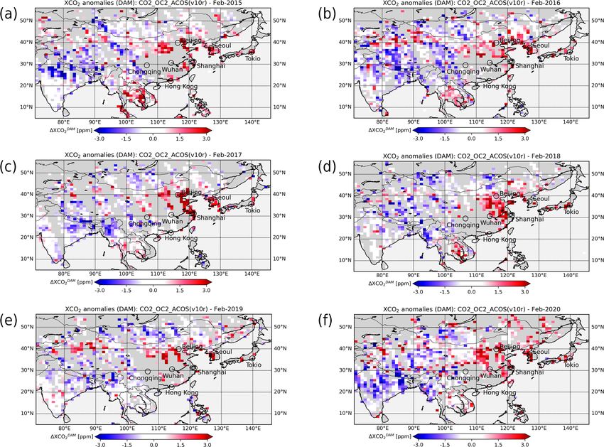
2142                     M. Buchwitz et al.: Satellite study of East China CO2 reduction during the COVID-19 pandemic

emissions (e.g. Ciais et al., 2014, 2015; Pinty et al., 2017,        ing constant emissions, the average relative (COVID-19 re-
2019; Crisp et al., 2018; Matsunaga and Maksyutov, 2018;             lated) change during January–April 2020 is therefore approx-
Janssens-Maenhout et al., 2020).                                     imately 7 % ± 4 % (0.242/3.3 ± 0.14/3.3). This agrees rea-
   Retrievals of XCO2 from the satellite sensors SCIA-               sonably well with the estimate reported in Liu et al. (2020),
MACHY/ENVISAT (Burrows et al., 1995; Bovensmann                      which is 9.3 % for China during the first quarter of 2020 com-
et al., 1999; Reuter et al., 2010, 2011) and TANSO-                  pared to the same period in 2019. Liu et al. (2020) also in-
FTS/GOSAT (Kuze et al., 2016) and from the Orbiting Car-             dicate some challenges in terms of interpreting CO2 emis-
bon Observatory-2 (OCO-2) satellite (Crisp et al., 2004; El-         sion reductions as being caused by COVID-19, e.g. the fact
dering et al., 2017; O’Dell et al., 2012, 2018) have been used       that the first months of 2020 were exceptionally warm across
in recent years to obtain information on natural CO2 sources         much of the Northern Hemisphere. CO2 emissions associ-
and sinks (e.g. Basu et al., 2013; Chevallier et al., 2014;          ated with home heating may have therefore been somewhat
Chevallier, 2015; Reuter et al., 2014a, 2017c; Schneising et         lower than for the same period in 2019, even without the dis-
al., 2014; Houweling et al., 2015; Kaminski et al., 2017; Liu        ruption in economic activities and energy production caused
et al., 2017; Eldering et al., 2017; Yin et al., 2018; Palmer        by COVID-19 and related lockdowns.
et al., 2019; Miller and Michalak, 2020), on anthropogenic              Sussmann and Rettinger (2020) studied ground-based
CO2 emissions (e.g. Schneising et al., 2008, 2013; Reuter            remote-sensing XCO2 retrievals of the Total Carbon Col-
et al., 2014b, 2019; Nassar et al., 2017; Schwandner et al.,         umn Observing Network (TCCON) to find out whether re-
2017; Matsunaga and Maksyutov, 2018; Miller et al., 2019;            lated atmospheric concentration changes may be detected
Labzovskii et al., 2019; Wu et al., 2020; Zheng et al., 2020a;       by the TCCON and brought into agreement with bottom-up
Ye et al., 2020), and for other applications such as climate         emission-reduction estimates. Our study is one of the first
model assessments (e.g. Lauer et al., 2017; Gier et al., 2020)       attempts to determine whether COVID-19-related regional-
or data assimilation (e.g. Massart et al., 2016).                    scale CO2 emission reductions can be detected using exist-
   Here we use an ensemble of satellite retrievals of XCO2           ing space-based observations of XCO2 . Tohjima et al. (2020)
to determine whether COVID-19-related regional-scale (here           inferred estimates of China’s CO2 emissions from modelled
∼ 20002 km2 ) CO2 emission reductions can be detected and            and observed ratios of CO2 and methane (CH4 ) surface con-
quantified using the current space-based observing system.           centrations at Hateruma Island, Japan. They report for China
This is important in order to establish the capabilities of cur-     fossil fuel emission reductions of 32 ± 12 % and 19 ± 15 %
rent satellites, which have been optimized to obtain infor-          for February and March 2020, respectively, which is about
mation on natural carbon sources and sinks but not to ob-            10 % higher compared to the results shown in Le Quéré et
tain information on anthropogenic emissions. Nevertheless,           al., 2020 (see Table 1 of Tohjima et al., 2020). From model
data from existing satellites have already been used to as-          sensitivity simulations they conclude that even a 30 % re-
sess anthropogenic emissions (see publications cited above).         duction of China’s fossil fuel CO2 emissions would only
These assessments and the assessment presented in this pub-          result in a 0.8 ppm XCO2 reduction over China and that it
lication are relevant for future satellites focussing on anthro-     therefore would be very challenging to detect any COVID-
pogenic emissions, such as the planned European Coperni-             19-related signal with the existing remote-sensing satellites
cus Anthropogenic CO2 Monitoring (CO2M) mission (e.g.                GOSAT and OCO-2. Their conjecture has essentially been
ESA, 2019; Kuhlmann et al., 2019; Janssens-Maenhout et               confirmed by Chevallier et al. (2020). They used XCO2 from
al., 2020), which is based on the CarbonSat concept (Bovens-         OCO-2 in combination with other data sets and the modelling
mann et al., 2010; Velazco et al., 2011; Buchwitz et al., 2013;      of CO2 emission plumes of localized CO2 sources to obtain
Pillai et al., 2016; Broquet et al., 2018; Lespinas et al., 2020).   estimates of CO2 emissions focussing on several COVID-
   We focus on China because regional-scale COVID-19-                19-relevant regions such as China, Europe, India and the
related CO2 emission reductions are expected to be largest           USA. They concluded that these places have not been well
there early in the pandemic (Le Quéré et al., 2020; Liu              observed by the OCO-2 satellite because of frequent or per-
et al., 2020). Satellite data have been used to estimate             sistent cloud conditions and they give recommendations for
China’s CO2 emissions during the COVID-19 pandemic as                future carbon-monitoring systems. Zeng et al. (2020) used
shown in Zheng et al. (2020b), but that study inferred CO2           modelling, GOSAT XCO2 and other data sets. They conclude
reductions from retrievals of nitrogen dioxide (NO2 ) not            that GOSAT is able to detect a short-term global mean XCO2
using XCO2 . Estimates of emission reductions have also              anomaly decrease of 0.2–0.3 ppm after temporal averaging
been derived from bottom-up statistical assessments of fos-          (e.g. monthly), but for East China they could not identify
sil fuel use and other economic indicators. According to             a statistically robust COVID-19-related anomaly. Satellite-
Le Quéré et al. (2020), China’s CO2 emissions decreased              derived results related to this application are also provided in
by 242 Mt CO2 (uncertainty range 108–394 Mt CO2 ) during             the internet (e.g. ESA-NASA-JAXA, 2020).
January–April 2020. As China’s annual CO2 emissions are                 Regional-scale reductions of tropospheric NO2 columns
approximately 10 Gt CO2 yr−1 (Friedlingstein et al., 2019),          have been reported for China (e.g. Zhang et al., 2020;
i.e. approximately 3.3 Gt CO2 in a 4-month period assum-             Bauwens et al., 2020), but for CO2 such an assessment is

Atmos. Meas. Tech., 14, 2141–2166, 2021                                               https://doi.org/10.5194/amt-14-2141-2021
M. Buchwitz et al.: Satellite study of East China CO2 reduction during the COVID-19 pandemic                                2143

more challenging because of small XCO2 changes on top of a         riod would then suggest (depending on uncertainty) that an
large background. For example, over extended anthropogenic         emission reduction during the COVID-19 period has been
source areas such as East China, the XCO2 enhancement due          detected.
to anthropogenic emissions is typically only approximately            The structure of our paper reflects this procedure: in the
1–2 ppm (0.25 %–0.5 % of 400 ppm) or even less (see e.g.           Data section (Sect. 2) we present the satellite and model in-
Schneising et al., 2008, 2013; Hakkarainen et al., 2016, 2019;     put data used for this study. In the Methods section (Sect. 3)
Chevallier et al., 2020; Tohjima et al., 2020; and this study).    we present the analysis method, which consists of two main
A 10 % emission reduction would therefore only change the          steps. The purpose of the first step is to isolate the East
regional XCO2 enhancement by 0.1 to 0.2 ppm. This is be-           China FF emission signal from the XCO2 satellite retrievals.
low the single measurement precision of current satellite          This is done by subtracting appropriate XCO2 background
XCO2 data products (at footprint size, i.e. 10.5 km diameter       values from the XCO2 retrievals to obtain XCO2 anoma-
for GOSAT (Kuze et al., 2016) and 1.3 × 2.3 km2 for OCO-           lies, 1XCO2 . We use two methods to compute 1XCO2 .
2 (O’Dell et al., 2018)), which is about 1.8 ppm (1σ ) (e.g.       We describe one method, the DAM method, in detail in
Dils et al., 2014; Kulawik et al., 2016; Buchwitz et al., 2015,    Sect. 3.1 and only shortly explain the second method (TmS
2017a; Reuter et al., 2020) for GOSAT and around 1 ppm for         method), referring for details to Appendix A. In the second
OCO-2 (Wunch et al., 2017; Reuter et al., 2019). In our study      step (Sect. 3.2) we compute estimates of East China monthly
we focus on XCO2 monthly averages. Averaging reduces the           FF CO2 emissions from the XCO2 anomalies. These emis-
noise of the satellite retrievals (e.g. Kulawik et al., 2016)      sion estimates are then used to compute the OND anomalies
but also eliminates day-to-day XCO2 variations (e.g. Agustí-       explained above. In Results and discussion section (Sect. 4)
Panareda et al., 2019), which cannot be interpreted using our      we present and discuss the results, i.e. the application of the
simple analysis methods. The accuracy of the East China            described methods to the satellite data. A summary and con-
satellite XCO2 retrievals averaged over monthly timescales         clusions are given in Sect. 5.
is difficult to assess because of limited reference data. The
validation of the satellite data products is primarily based
on comparisons with ground-based XCO2 retrievals from the          2     Data
TCCON, a relatively sparse network with an uncertainty of
about 0.4 ppm (Wunch et al., 2010).                                In this section, we present a short overview about the input
   The purpose of this study is to investigate – using satellite   data used for this study.
XCO2 retrievals – if satellite-derived East China fossil fuel
(FF) CO2 emissions in 2020 (COVID-19 period) differ sig-           2.1    Satellite XCO2 retrievals
nificantly compared to pre-COVID-19 periods. Ideally, we
would like to know by how much emissions have been re-             This study uses four satellite XCO2 Level 2 (L2) data prod-
duced due to COVID-19. This question, however, cannot be           ucts. An overview about these data sets is provided in Ta-
answered using only satellite data because they do not con-        ble 1. The first product listed in Table 1 is the latest ver-
tain any information on how much would have been emitted           sion of the bias-corrected OCO-2 XCO2 product delivered
without COVID-19. Instead, we aim at answering the follow-         to the Goddard Earth Science Data and Information Services
ing question: are satellite-derived East China FF CO2 emis-        Center (GES DISC) by the OCO-2 team (ACOS v10r Lite).
sions early in the pandemic (here: January–May 2020) sig-          The other three satellite XCO2 data sets are different ver-
nificantly lower compared to pre-COVID-19 periods?                 sions of the GOSAT XCO2 product derived using retrieval
   To answer this question, we analyse relative differences of     algorithms developed by groups at the University of Leices-
estimates of East China monthly FF emissions during dif-           ter, UK (UoL-FP v7.3); the SRON Netherlands Institute for
ferent time periods. We focus on October-to-May periods,           Space Research (RemoTeC v2.3.8); and the University of
and we refer to different periods via the year where a period      Bremen, Germany (FOCAL v1.0).
ends; i.e. we call the period October 2019 to May 2020 “year          The XCO2 estimates derived from OCO-2 (e.g. O’Dell
2020 period” or simply “2020”, the period October 2018 to          et al., 2018) and GOSAT (e.g. Kuze et al., 2016) obser-
May 2019 is called 2019, etc. Specifically, we compute and         vations are complementary because these two spacecraft
analyse differences of monthly emissions in the year 2020          use different sampling strategies. OCO-2 has been operat-
period relative to previous year 2016 to 2019 periods; i.e. we     ing since September 2014. Its spectrometers collect about
use four periods for comparison with the year 2020 period.         85 000 cloud-free XCO2 soundings each day along a narrow
To focus on the COVID-19 aspect, we subtract for each pe-          (< 10 km) ground track as it orbits the Earth 14.5 times each
riod the October-to-December (OND) mean value, and we              day from its sun-synchronous 13:36 (local time) orbit. The
refer to these time series as “OND anomalies”. These OND           OCO-2 soundings provide continuous measurements with
anomalies are time series at monthly resolution of the rela-       relatively high spatial resolution (1.3 × 2.3 km2 ) along each
tive emission difference between different periods relative to     track, but the individual ground tracks are separated by al-
OND. Negative OND anomalies during the COVID-19 pe-                most 25◦ longitudes in any given day. This spacing is reduced

https://doi.org/10.5194/amt-14-2141-2021                                            Atmos. Meas. Tech., 14, 2141–2166, 2021
2144                            M. Buchwitz et al.: Satellite study of East China CO2 reduction during the COVID-19 pandemic

Table 1. Overview of the satellite XCO2 Level 2 (L2) input data products.

      Satellite     Algorithm         Product       Product ID                  References                    Data provider and data access information
                                      version
      OCO-2         ACOS              v10r          CO2_OC2_ACOS                O’Dell et al. (2018),         Product OCO2_L2_Lite_FP 10r obtained
                                                                                Kiel et al. (2019),           from NASA’s Earthdata GES DISC website:
                                                                                Osterman et al.               https://disc.gsfc.nasa.gov/datasets?keywords=
                                                                                (2020)                        OCO-2%20v10r&page=1 (last access:
                                                                                                              15 August 2020)
      GOSAT         UoL-FP            v7.3          CO2_GOS_OCFP                Cogan et al. (2012),          Generated by Univ. Leicester (contact: Antonio
                                                                                Boesch et al. (2019)          Di Noia: adn9@leicester.ac.uk) and available
                                                                                                              via the CDS∗
      GOSAT         RemoTeC           v2.3.8        CO2_GOS_SRFP                Butz et al. (2011),           Generated by SRON (contact: Lianghai Wu:
                                                                                Wu et al. (2019)              l.wu@sron.nl) and available via the CDS∗
      GOSAT         FOCAL             v1.0          CO2_GOS_FOCA                Noël et al. (2020)            Generated by Univ. Bremen and available on
                                                                                                              request (contact: Stefan Noël:
                                                                                                              stefan.noel@iup.physik.uni-bremen.de)
    ∗ Products are available via the Copernicus Climate Data Store (CDS, https://cds.climate.copernicus.eu/cdsapp#!/dataset/satellite-carbon-dioxide?tab=overview (last
    access: 23 September 2020)) currently until end of 2019. Year 2020 data will be made available via the CDS in mid-2021 but are available from the authors on request (see
    contact information).

to approximately 1.5◦ longitude after a 16 d ground track re-                               et al., 2014b, 2019; Nassar et al., 2017), but extracting this
peat cycle. GOSAT has been returning 300 to 1000 cloud-                                     information requires appropriate data processing and analy-
free XCO2 soundings each day since April 2009. Its TANSO-                                   sis. For a strong (net) source region XCO2 is typically higher
FTS spectrometer collects soundings with 10.5 km diameter                                   compared to its surrounding area. Our method is based on
surface footprints, separated by approximately 250 km along                                 computing and subtracting XCO2 background values. The
and across its ground track at it orbits from north to south                                purpose of this background correction is to isolate the re-
across the sunlit hemisphere.                                                               gional emission signal by removing large-scale spatial and
                                                                                            day-to-day temporal XCO2 variations, which cannot be dealt
2.2    Model CO2 data                                                                       with in our simple data-driven method to estimate emissions.
                                                                                               XCO2 varies temporally and spatially (e.g. Agustí-
We use data from NOAA’s (National Oceanic and Atmo-                                         Panareda et al., 2019; Reuter et al., 2020; Gier et al., 2020),
spheric Administration) CO2 assimilation system, Carbon-                                    for example, due to quasi-regular uptake and release of CO2
Tracker (CT2019) (Jacobson et al., 2020; Peters et al., 2007),                              by the terrestrial biosphere, which results in a strong sea-
to define the relationship between XCO2 anomalies and fos-                                  sonal cycle, especially over northern mid- and high latitudes.
sil fuel emissions. CarbonTracker is a global atmospheric in-                               Compared to fluctuations originating from the interaction
verse model that assimilates atmospheric CO2 measurements                                   of the terrestrial biosphere and the atmosphere, the spatio-
to produce modelled fields of atmospheric CO2 mole frac-                                    temporal XCO2 variations due to anthropogenic fossil fuel
tions by adjusting land biosphere and ocean CO2 surface                                     (FF) CO2 emissions are typically much smaller (e.g. 1 ppm
fluxes. An overview about CT2019 set is provided in Ta-                                     compared to 10 ppm; Schneising et al., 2008, 2013, 2014;
ble 2, including references and access information. In short,                               Agustí-Panareda et al., 2019).
CarbonTracker has a representation of atmospheric transport                                    A method used for background correction is the one de-
based on weather forecasts, as well as modules represent-                                   scribed in Hakkarainen et al. (2019; see also Hakkarainen
ing air–sea exchange of CO2 , photosynthesis and respiration                                et al., 2016, for a first publication of that method). We use
by the terrestrial biosphere, and release of CO2 to the atmo-                               two different methods for background correction. We refer
sphere by fires and combustion of fossil fuels.                                             to these methods as “daily anomalies via (latitude band) me-
                                                                                            dians” (DAM), which is essentially identical with the method
                                                                                            described in Hakkarainen et al. (2019), and “target minus sur-
3     Methods                                                                               rounding” (TmS).
                                                                                               Hakkarainen et al. (2019) applied their method to the
3.1    Methods to compute XCO2 anomalies (1XCO2 )                                           OCO-2 Level 2 XCO2 data product to filter out trends and
                                                                                            seasonal variations in order to isolate CO2 source/sink sig-
Satellite XCO2 retrievals contain information on anthro-                                    nals. For background correction, Hakkarainen et al. (2019)
pogenic CO2 emissions (e.g. Schneising et al., 2013; Reuter

Atmos. Meas. Tech., 14, 2141–2166, 2021                                                                            https://doi.org/10.5194/amt-14-2141-2021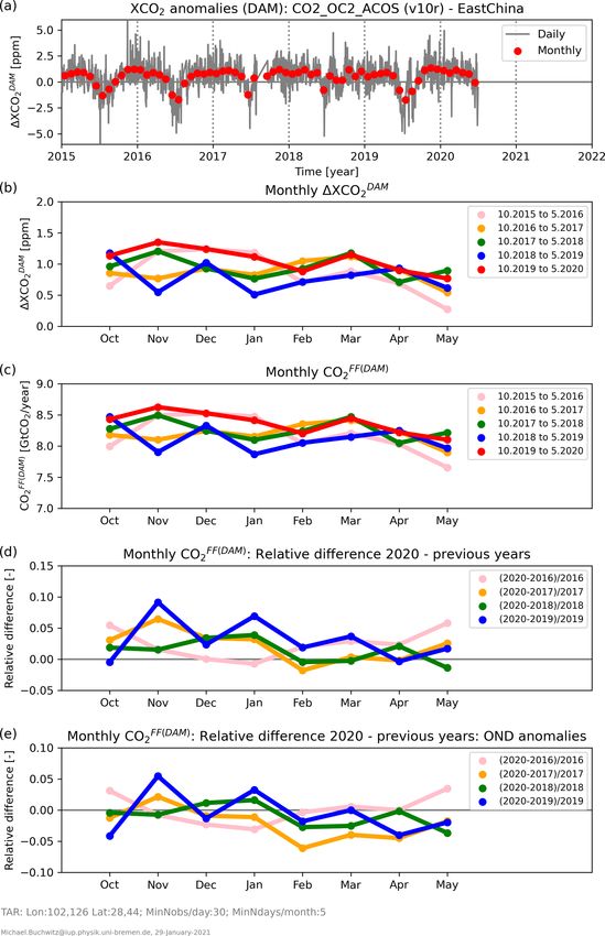
M. Buchwitz et al.: Satellite study of East China CO2 reduction during the COVID-19 pandemic 2145
Table 2. Overview of the CarbonTracker CT2019 data set. For this study we used data from the period January 2015 to December 2018.
Model/version Details Reference Access
CarbonTracker Atmospheric CO2 mole fraction profiles Jacobson et al. (2020), DOI: CarbonTracker CT2019,
CT2019 (spatio-temporal sampling: 3◦ × 2◦ , https://doi.org/10.25925/39m3-6069 http://carbontracker.noaa.gov
3-hourly) and CO2 fluxes (spatio- (last access: 22 July 2020)
temporal sampling: 1◦ × 1◦ , 3-hourly)
Table 3. Corner coordinates of the East China target region as anal- and the desired estimates of the target region fossil fuel (FF)
ysed in this study. emissions. To develop a method to convert the XCO2 anoma-
lies, 1XCO2 , to FF emission estimates, COFF 2 , we use an ex-
Region ID Comments Latitude Longitude isting model data set, the CarbonTracker CT2019 data set de-
range range scribed in Sect. 2.2, which contains atmospheric CO2 fields
(◦ N) (◦ E) and corresponding CO2 surface fluxes during 2015–2018.
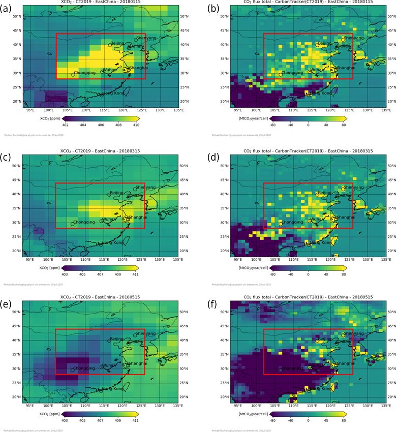
East China Target region for DAM 28–44 102–126 Figure 1 shows CT2019 XCO2 maps (left) and corre-
and TmS methods sponding surface CO2 flux maps (right) for selected days in
the January-to-May-2018 period. The XCO2 has been com-
Extended region for 18–54 93–135
TmS method
puted by vertically integrating the CT2019 CO2 vertical pro-
files (weighted with the surface pressure normalized pressure
change over each layer). The model data are sampled at lo-
cal noon, which is close to the overpass time of the satellite
calculate daily medians for 10◦ latitude bands and linearly data sets used here. The spatio-temporal sampling of a spe-
interpolate the resulting values to each OCO-2 data point. In- cific satellite XCO2 data product is not considered here; i.e.
stead of interpolation, we compute the median around each we use the CT2019 data set independent of any satellite data
latitude (running median) using a latitude band width of product apart for the sampling at local noon. As can be seen
±15◦ . We use a larger width compared to Hakkarainen et from Fig. 1, XCO2 is clearly elevated over the East China tar-
al. (2019), as we also apply our method to GOSAT data, get region (red rectangle) relative to its surrounding region on
which are much sparser than OCO-2 data. Our investigations 15 January 2018 (Fig. 1a) and on 15 March 2018 (Fig. 1c).
showed that the width of the latitude band is not critical. The On 15 May 2018 (Fig. 1e) the target region and parts of the
band needs to be wide enough to contain a statistically sig- surrounding region contain large areas of lower-than-average
nificant sample but narrow enough to resolve large latitudi- XCO2 , a pattern which primarily results from carbon uptake
nal gradients in CO2 . We subtract the corresponding median by vegetation during the growing season, which starts in east-
from each single XCO2 observation in the original Level 2 ern China around May each year. The CO2 fluxes, which are
XCO2 data product files to obtain a data set of XCO2 anoma- shown on the right-hand side panels of Fig. 1, show simi-
lies, 1XCODAM2 . lar spatial pattern as the XCO2 maps, but due to atmospheric
In order to verify that our results do not critically depend transport and the long lifetime of atmospheric CO2 there is
on the details of one method, we also use the second TmS no one-to-one correspondence between atmospheric XCO2
method. Here we obtain the background by averaging XCO2 and surface emissions. The CO2 fluxes are the sum of several
in a region surrounding the target region (see Table 3 for the contributing fluxes including FF emissions, biogenic fluxes
latitude and longitude corner coordinates of the target and its and other fluxes (fires, oceans).
surrounding region). Figure 2a shows time series obtained by applying the
We call these background-corrected XCO2 retrievals DAM method to CT2019 XCO2 for the East China target
XCO2 anomalies, and satellite-derived maps and time se- region. The CT2019 data set not only contains atmospheric
ries of these XCO2 anomalies are presented and discussed in CO2 concentrations but also its components due to fossil fuel
Sect. 4.1. These XCO2 anomalies are then used to compute (FF) emissions and biogenic (BIO) and other fluxes. From
East China FF CO2 emission estimates, COFF 2 , as described the CT2019 data set we computed total XCO2 (TOT) and its
in the following subsection. FF and BIO components. From these components we sub-
tracted the background using the DAM method, and the cor-
3.2 Computation of emission estimates (COFF
2 ) responding monthly 1XCODAM time series are shown in
2
Fig. 2a. As can be seen from Fig. 2a, total 1XCODAM 2 (black
To determine whether satellite XCO2 retrievals can provide line) is dominated by its FF (red line) and BIO (green line)
information on relative changes of anthropogenic CO2 emis- components (their sum, i.e. FF + BIO (grey line), is close to
sions for the East China target region, we must establish TOT (black line)). As can also be seen, FF emissions for East
a relationship between the XCO2 anomalies (see Sect. 3.1)
https://doi.org/10.5194/amt-14-2141-2021 Atmos. Meas. Tech., 14, 2141–2166, 2021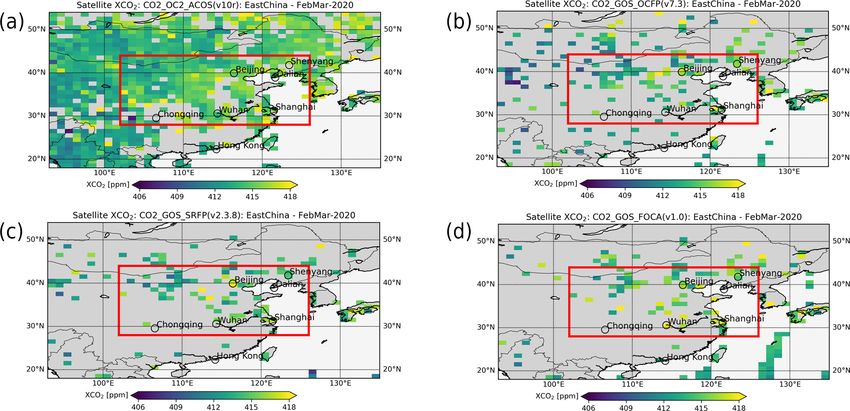
2146                     M. Buchwitz et al.: Satellite study of East China CO2 reduction during the COVID-19 pandemic

Figure 1. CT2019 XCO2 (a, c, e, in ppm) and corresponding CO2 surface fluxes (b, d, f, in Mt CO2 yr−1 per cell) for 15 January 2018 (a, b),
15 March 2018 (c, d) and 15 May 2018 (e, f). The red rectangle encloses the East China target region as defined for this study.

China (red line) are larger than the BIO fluxes (green line) at         sions. As a consequence, total 1XCODAM    2     (black line) gets
least during October to April. During May to September the              negative. During these months, the total anomaly (black line)
BIO fluxes are negative due to uptake of atmospheric CO2                is closer to BIO (green line) than to FF (red line).
by the terrestrial biosphere, and their absolute value is on the           The task for the satellite inversion is to obtain estimates of
same order or may even significantly exceed the FF emis-                East China FF CO2 emissions from the satellite-derived (to-

Atmos. Meas. Tech., 14, 2141–2166, 2021                                                   https://doi.org/10.5194/amt-14-2141-2021
M. Buchwitz et al.: Satellite study of East China CO2 reduction during the COVID-19 pandemic                                         2147

Figure 2. Results obtained by applying the DAM method to CT2019 XCO2 for East China. (a) Different monthly 1XCODAM         2   components:
total 1XCO2  DAM    (TOT) and its FF (red) and biogenic (BIO, green) components and their sum (FF + BIO). The non-shaded time periods
October to May indicate the periods analysed in this publication. (b) East China October-to-May FF CO2 emissions (red dots) and estimated
               FF(DAM)
emissions CO2            (black crosses) as obtained from total 1XCODAM2    (TOT as shown in panel a) using the formula shown in panel (b).
(c) Scatter plot of estimated versus true (i.e. CT2019) FF emissions. (d) Relative difference of estimated and true emissions.

tal) XCO2 anomalies, 1XCODAM    2     (black line in Fig. 2a). To       emissions agree reasonably well with the true emissions. The
determine to what extent this is possible, we fitted CT2019             linear correlation coefficient R is 0.83 (see Fig. 2c), and the
1XCODAM  2    (i.e. the quantity that we can also obtain from           relative difference in terms of mean and standard deviation
satellites) to the East China CT2019 FF CO2 emissions                   is 0.2 % ± 5 % (see Fig. 2d). However, for individual months
(which are the known true emissions in this model data as-              the error can be as large as 10 %. From this we conclude that
sessment exercise). The results are shown in Fig. 2b for                the (approximately 2σ ) uncertainty of our method is approx-
October-to-May periods. The estimated emissions (black                  imately 10 %.
crosses) have been obtained via a linear fit of 1XCODAM     2              A similar figure but generated using the TmS method is
to the CT2019 FF emissions (red dots). The two parameters               shown in Appendix A as Fig. A1. As can be seen, the re-
of the linear fit are also shown in Fig. 2b: scaling factor A           sults shown in Fig. A1b to d are similar to the ones shown
(= 0.90) and offset B (= 7.41). As can be seen, the estimated           in Fig. 2b to d, but the linear correlation is slightly worse

https://doi.org/10.5194/amt-14-2141-2021                                                   Atmos. Meas. Tech., 14, 2141–2166, 2021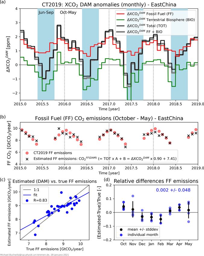
2148 M. Buchwitz et al.: Satellite study of East China CO2 reduction during the COVID-19 pandemic
and the errors are slightly larger. In contrast, the time se-
ries shown in panel (a) differ significantly. This is because of
the different background corrections used for the two meth-
ods. But despite these significant differences the quality of
the derived emissions is similar (the standard deviation of
the monthly biases is 5.5 % for TmS and 4.8 % for DAM;
see panel d). Nevertheless, the DAM method gives slightly
better results compared to the TmS method, and this is also
confirmed by applying both methods to the satellite data (see
Sect. 4). Therefore, the DAM method is our baseline method,
and we focus on results obtained with the DAM method.
It is perhaps surprising that the offset (fit parameter B; see
above) is so large (7.41 for DAM and 7.63 for TmS). Prob- Figure 3. DAM XCO2 anomaly map at 1◦ × 1◦ resolution gener-
ated from OCO-2 Level 2 XCO2 (v10r, land) for 2015 to 2019.
ably one would assume that the XCO2 anomalies 1XCO2
are directly proportional to the target region fossil fuel emis-
sions, i.e. one would assume that FF is (approximately) cantly different, taking into account the year-to-year variabil-
equal to a constant multiplied by 1XCO2 (no offset added) ity, which we use to obtain uncertainty estimates.
(for example, for FF = 8 Gt CO2 yr−1 and 1XCO2 = 2 ppm The methods described in this section have been applied
one would have expected that the conversion factor is 4 to convert satellite-derived target region XCO2 anomalies,
Gt CO2 yr−1 ppm−1 ). In that case, as we are only inter- 1XCO2 , into estimated target region FF CO2 emissions,
ested in relative changes in emissions, we would not need COFF 2 . How this has been done using the DAM method for
to know the exact value of the scaling factor. However, background correction is explained in the following Sect. 4,
when analysing the satellite data, we found that 1XCO2 where we refer for the corresponding TmS method results to
is around 2 ppm for January but decreases in subsequent Appendix A.
months, nearly approaching zero in May (which is consistent
with the CT2019 results shown in Fig. 2a). As anthropogenic
emissions are not expected to change that much within a few 4 Results and discussion
months (and zero emissions around May are not realistic at
all), we concluded that the simple proportionality assump- In this section, we present results obtained by applying the
tion does not hold. To investigate this we used the CT2019 DAM method (see Methods Sect. 3.1) to the satellite data to
data set to test and improve our method, and the results are obtain XCO2 anomalies from which we derive FF emission
reported in this section. We applied our method to CT2019 estimates (see Methods Sect. 3.2).
XCO2 (as shown in Fig. 2) and compared the retrieved FF
values with the (true) CT2019 FF values. We found large dif- 4.1 Application of the DAM method to satellite XCO2
ferences, which could be significantly reduced by adding an retrievals
offset to the linear fit as discussed above. The reason for the
The DAM method has been applied to the OCO-2 and
large offset is the influence of the biosphere. Around May the
GOSAT satellite XCO2 data products listed in Table 1. Fig-
uptake of atmospheric CO2 due to the biosphere is so large
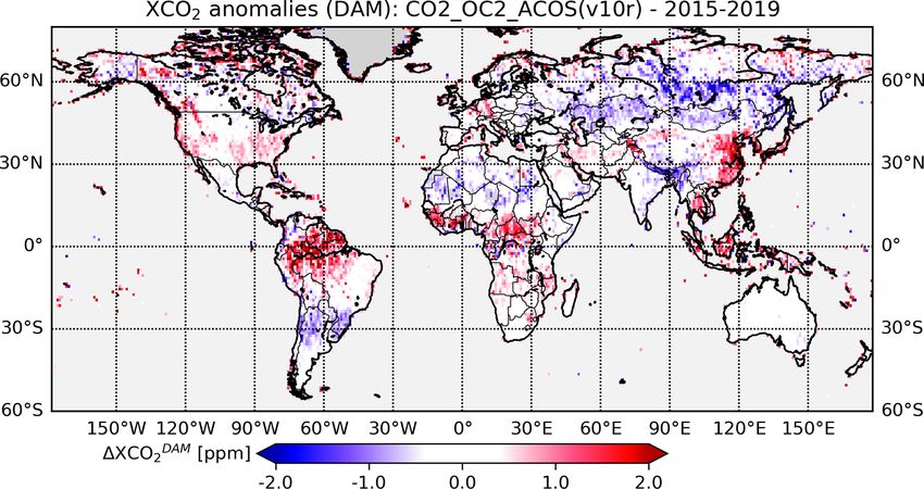
ure 3 shows a global OCO-2 DAM XCO2 anomaly map at
that 1XCO2 is close to zero – but the FF emissions are not –
1◦ × 1◦ resolution for the period 2015–2019. A similar map
and the East China target region is essentially carbon neutral
is shown in Hakkarainen et al. (2019; see their Fig. 3, top
or even a net sink (see also Fig. 1).
panel). The degree of agreement confirms the finding re-
As explained, scaling factor A and offset B are obtained
ported in Sect. 3.1 that the generation of these anomaly maps
empirically via a linear fit using CT2019 data (Fig. 2b) and
does not critically depend on how exactly the median is com-
used for the conversion of the satellite XCO2 anomalies dur-
puted and used to subtract the background. Hakkarainen et
ing the entire time period January 2015 to May 2020 (as will
al. (2019) discuss their OCO-2-derived maps in quite some
be shown in Sect. 4). As can be seen from Fig. 2b and c,
detail also in terms of seasonal averages and comparisons
the retrieval biases are within ±10 % during 2015–2018. We
with model simulations. They show that positive anomalies
assume in our study that the same conversion is also appro-
correspond to fossil fuel combustion over major industrial ar-
priate for 2019 and 2020. However, it cannot be ruled out that
eas including China. Their seasonal maps (see their Fig. 4)
2019 or 2020 were significantly different compared to previ-
show a strong positive anomaly over East China (similar
ous years with respect to aspects relevant for our study. To
to that shown here in Fig. 3) except for the June–August
address this, we compare the period October 2019 to May
(JJA) summer season, where the XCO2 anomaly can be neg-
2020 results with the corresponding results from previous
ative. This is consistent with the CT2019 results presented in
October-to-December periods to find out to what extent the
Sect. 3.2.
period of interest, i.e. October 2019 to May 2020, is signifi-
Atmos. Meas. Tech., 14, 2141–2166, 2021 https://doi.org/10.5194/amt-14-2141-2021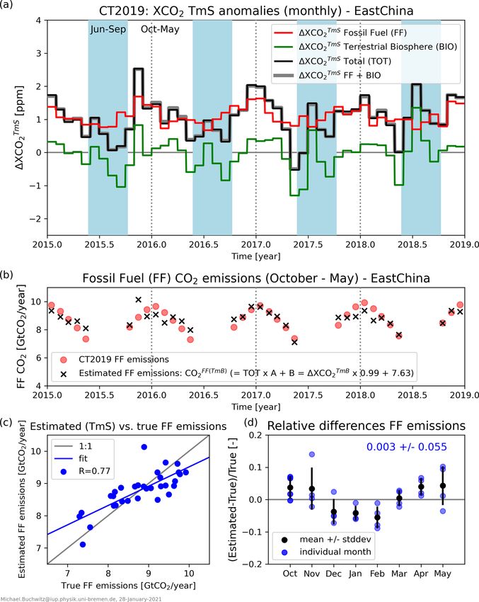
M. Buchwitz et al.: Satellite study of East China CO2 reduction during the COVID-19 pandemic                                     2149

                                                                      tial sampling of the target region is different for each prod-
                                                                      uct as only quality-filtered (i.e. good) data are shown and the
                                                                      quality filtering is algorithm specific (see references listed in
                                                                      Table 1).
                                                                         Figure 6 also shows as red rectangle the East China tar-
                                                                      get region as defined for this study (the geographical coordi-
                                                                      nates are listed in Table 3). The fossil fuel (FF) CO2 emis-
                                                                      sions of this target region are approximately 8 Gt CO2 yr−1 ;
                                                                      i.e. the selected target region covers approximately 80 %
                                                                      of the FF emissions of all of China, which are approxi-
                                                                      mately 10 Gt CO2 yr−1 (Le Quéré et al., 2018; Friedlingstein
                                                                      et al., 2019). In the following section we present East China
Figure 4. As Fig. 3 but for China and surrounding areas.              FF emission estimates as derived from the satellite XCO2
                                                                      anomalies during and before the COVID-19 period.

   A zoom into Fig. 3 is presented in Fig. 4, which shows             4.2     Emission estimates
more details for China and its surrounding area. As can be
seen from Fig. 4, 1XCODAM         is positive especially in the re-
                             2                                        Carbon dioxide fossil fuel emission estimates, COFF2 , have
gion between Beijing, Wuhan and Hong Kong, with the high-
                                                                      been derived from the XCO2 anomalies, 1XCO2 , computed
est values in the area between Beijing and Shanghai. This
                                                                      for each of the four satellite XCO2 data products listed in
positive anomaly indicates that this region is a strong CO2
                                                                      Table 1. In this section the emission results are presented
source region as also discussed in Hakkarainen et al. (2019).
                                                                      and discussed. We focus on results based on 1XCO2 derived
As already explained, there is no one-to-one correspondence
                                                                      with the DAM method and refer to Appendix A for results
(especially not for every grid cell) between local XCO2
                                                                      based on the TmS method.
anomalies and local CO2 emissions (or uptake) because the
emitted CO2 is transported and mixed in the atmosphere.
Furthermore, the satellite data are typically sparse due to           4.2.1    Emission estimates from NASA’s OCO-2 (version
strict quality filtering to avoid potential XCO2 biases, for ex-               10r) XCO2
ample, due to the presence of clouds. Cloud-contaminated
ground scenes are identified to the extent possible via the cor-      Figure 7 shows the results obtained by applying the DAM
responding retrieval algorithm (see references listed in Ta-          method to product CO2_OC2_ACOS (see Table 1) for the
ble 1) and flagged to be bad and are therefore not used for           East China target region for the period January 2015 to May
this analysis. The sparseness of the satellite data set is obvi-      2020 (the TmS version of this figure is shown as Fig. A2 in
ous from Fig. 5, which shows OCO-2 DAM XCO2 anomaly                   Appendix A). Figure 7a shows daily DAM XCO2 anomalies
maps for February during the 6 years 2015 to 2020.                    as a thin grey line and the corresponding monthly averages
   A key difference between the OCO-2 and the GOSAT                   as red dots. The amplitude (approximately ±1 ppm) and time
data products is the different sampling of the target region,         dependence (e.g. the minimum in the middle of each year)
with GOSAT having much sparser coverage compared to                   are similar to that for CT2019 (Fig. 2a black line). To ensure
OCO-2. This is illustrated in Fig. 6, which shows February-           that there are a sufficiently large number of observations per
to-March-2020 averages of the OCO-2 XCO2 data product                 month, two criteria need to be fulfilled: There must be a min-
(Fig. 6a) and the three GOSAT data products (Fig. 6b–d) at            imum number of days per month (here: 5) and a minimum
1◦ × 1◦ resolution. The OCO-2 product shown in Fig. 6a is             number observations per day (here: 30). The latter criterion
NASA’s OCO-2 operational Atmospheric CO2 Observations                 is also relevant for the daily data shown in Fig. 7(a) (grey
from Space (ACOS) algorithm version 10r bias-corrected                line). We also used other combinations of these two parame-
XCO2 product (the so-called Lite product), which is re-               ters (as shown below, e.g. Fig. 9).
ferred to in this publication via the product identifier (ID)            Figure 7b shows monthly 1XCODAM         2     for different
CO2_OC2_ACOS. The three GOSAT XCO2 products are                       October-to-May periods, and Fig. 7c shows the correspond-
                                                                                                          FF(DAM)
(see details and references as given in Table 1) the Univer-          ing estimated FF emissions, CO2             . Figure 7d shows
sity of Leicester’s GOSAT product (ID CO2_GOS_OCFP;                   relative differences of the time series shown in Fig. 7c. For
Fig. 6b), SRON Netherlands Institute for Space Research               example, the blue data are referred to as “(2020–2019)/2019”
GOSAT product (CO2_GOS_SRFP; Fig. 6c), and University                 in Fig. 7d, where 2019 refers to the blue data in Fig. 7c,
of Bremen’s GOSAT product (CO2_GOS_FOCA; Fig. 6d)                     which corresponds to the period ending in May 2019. Shown
as retrieved with the Fast atmOspheric traCe gAs retrievaL            are differences of year 2020 data (red in Fig. 7c) minus data
(FOCAL) retrieval algorithm initially developed for OCO-2             from previous periods; i.e. Fig. 7d shows to what extent 2020
(Reuter et al., 2017a, b). As can be seen from Fig. 6, the spa-       (strictly speaking the period October 2019–May 2020, i.e.

https://doi.org/10.5194/amt-14-2141-2021                                                Atmos. Meas. Tech., 14, 2141–2166, 2021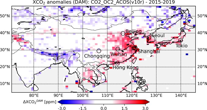
2150                      M. Buchwitz et al.: Satellite study of East China CO2 reduction during the COVID-19 pandemic

Figure 5. As Fig. 4 but for (a) February 2015 to (f) February 2020.

the period which ends in 2020) differs relative to previous              Figures 7 and 8 have been generated with the requirement
October-to-May periods.                                               that for each day at least 30 observations need to be available
   To find out if we can detect a difference between the              in the target region and for each month at least 5 d fulfilling
COVID-19 period and pre-COVID-19 periods, we subtract                 this 30 observations per day requirement. Figure 9 is similar
from each time series shown in Fig. 7d the October-to-                to Fig. 8 except that also results for additional combinations
December (OND) mean value. The corresponding time se-                 have been added, i.e. other combinations of minimum num-
ries are shown in Fig. 7e and are referred to as OND anoma-           ber of observations per day and minimum number of days
lies in the following. As can be seen from Fig. 7e, the OND           per month. As can be seen, the results depend somewhat on
anomalies vary within ±5 %. Values before January scatter             which combination of these parameters is used, but the en-
around zero as the mean value of OND anomalies is zero by             semble median and its uncertainty (royal blue symbols and
definition during October to December. In January the values          lines) are similar. The ensemble median values are similar
also scatter around zero. After January most values are nega-         and negative during February to May 2020. The large uncer-
tive, indicating reduced emissions compared to pre-COVID-             tainties (vertical lines; 1σ error estimates) reflect the scatter
19 periods. This can be seen more clearly in Fig. 8, where the        of the ensemble members. The errors bars (1σ ) overlap with
same data as in Fig. 7e are shown, but in addition the ensem-         the zero (i.e. no reduction) line, indicating that it cannot be
ble mean (light blue thick lines and dots) and median (royal          claimed with confidence that a significant drop of the emis-
blue thick lines and dots) has been added, including uncer-           sions during the COVID-19 period has been detected.
tainty estimates as computed from the standard deviation of
the ensemble members.

Atmos. Meas. Tech., 14, 2141–2166, 2021                                                https://doi.org/10.5194/amt-14-2141-2021
M. Buchwitz et al.: Satellite study of East China CO2 reduction during the COVID-19 pandemic 2151
Figure 6. (a) OCO-2 XCO2 (version 10r, product ID CO2_OC2_ACOS) over land at 1◦ × 1◦ resolution for February–March 2020. The red
rectangle encloses the investigated East China target region. (b–d) As panel (a) but for products CO2_GOS_OCFP (b), CO2_GOS_SRFP (c)
and CO2_GOS_FOCA (d) (see Table 1 for details).
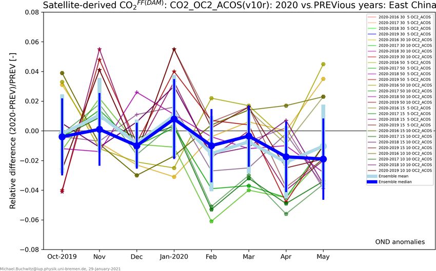
4.2.2 Emission estimates from GOSAT XCO2 data in Appendix A). The results obtained from the individual
products products (as shown in royal blue in Figs. 9–12) are shown
here using reddish colours (the corresponding numerical val-
The same analysis method as applied to NASA’s OCO- ues are listed in Table 4). Also shown in Fig. 13 is the mean of
2 data product (Sect. 4.2.1) has also been applied to the the ensemble members and its estimated uncertainty (in dark
three GOSAT XCO2 data products listed in Table 1. The blue); the corresponding numerical values are listed in the
results are shown in Fig. 10 for product CO2_GOS_OCFP, bottom row of Table 4. The ensemble mean suggests emis-
in Fig. 11 for product CO2_GOS_SRFP and in Fig. 12 for sion reductions by approximately 10 % ± 10 % in March and
product CO2_GOS_FOCA. The month-to-month variations April 2020. However, as can also be seen, there are signif-
are larger for these GOSAT products compared to OCO-2 icant differences across the ensemble of satellite data prod-
product (note the different scale of the y axes compared to ucts. For example, the analysis of the OCO-2 data suggests
Fig. 9). This is because GOSAT products are much sparser a much smaller emission reduction of only about 1 %–2 %.
compared to the OCO-2 product (as shown in Fig. 6) and Because of the large differences between the individual en-
because the single observation random error is larger for semble members it is concluded that the expected emission
GOSAT compared to OCO-2. As can be seen from a com- reduction cannot be reliably detected and accurately quanti-
parison of the results obtained for the three GOSAT prod- fied with our method.
ucts (Figs. 10–12), there are large differences among the
results obtained from these products. For example, product
CO2_GOS_OCFP (Fig. 10) suggests that the largest emis- 5 Summary and conclusions
sion reduction is in April, in contrast to the other two prod-
ucts. The large spread of the GOSAT results means that no We have analysed a small ensemble of satellite XCO2 data
clear conclusions can be drawn concerning East China emis- products to investigate whether a regional-scale reduction of
sion reductions during the COVID-19 period. atmospheric CO2 during the COVID-19 pandemic can be de-
tected for East China. Specifically, we analysed four XCO2
4.2.3 Ensemble mean and uncertainty data products from the satellites OCO-2 and GOSAT. For this
purpose, we used a simple data-driven approach, which in-
An overview about the results obtained from all four satellite volves the computation of XCO2 anomalies, 1XCO2 , using
data products using the DAM method is shown in Fig. 13 (the a method called DAM (daily anomalies via (latitude band)
corresponding TmS version of this figure is shown as Fig. A3 medians). This method, which is essentially identical with
https://doi.org/10.5194/amt-14-2141-2021 Atmos. Meas. Tech., 14, 2141–2166, 20212152 M. Buchwitz et al.: Satellite study of East China CO2 reduction during the COVID-19 pandemic
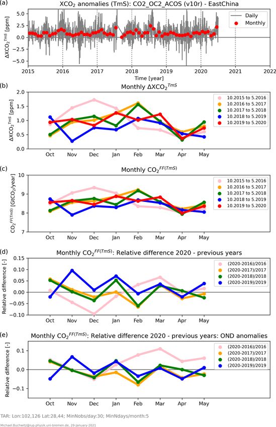
Figure 7. DAM analysis of the OCO-2 ACOS version 10r XCO2 product (CO2_OC2_ACOS) for the East China region from January 2015
to May 2020. (a) The thin grey line shows the daily DAM XCO2 anomalies, i.e. daily 1XCODAM
2 . The red dots are the corresponding
FF(DAM)
monthly values, which are also shown in panel (b) for different October–May periods. (c) As panel (b) but for CO2 , i.e. for the
estimated East China monthly FF emissions (see main text). The data for October 2019–May 2020 (10.2019–5.2020) are shown in red (see
FF(DAM)
annotation for other periods). (d) Relative CO2 differences for different periods. In blue, for example, the differences correspond
to the period 10.2019–5.2020 (shown in red in panel c) minus 10.2018–5.2019 (shown in blue in panel c). (e) As panel (d) but after the
October-to-December mean value (OND anomalies). The following parameters have been used to generate this figure: minimum number of
observations per day: 30; minimum number of days per month: 5.
Atmos. Meas. Tech., 14, 2141–2166, 2021 https://doi.org/10.5194/amt-14-2141-2021M. Buchwitz et al.: Satellite study of East China CO2 reduction during the COVID-19 pandemic 2153
FF(DAM)
Figure 8. Ensemble member CO2 OND anomalies derived from the satellite product CO2_OC2_ACOS. The thin lines and small
symbols show the same data also shown in the bottom panel of Fig. 7. The thick dots and lines show the corresponding ensemble median,
mean and scatter. The following parameters have been used to generate this figure (see also annotation): minimum number of observations
per day: 30; minimum number of days per month: 5.
Figure 9. The same as Fig. 8 but with additional combinations of minimum number of observations per day (30 as in Fig. 8 and in addition
50, 15 and 10) and minimum number of days per month (5 as in Fig. 8 and in addition 10) (see annotation).
https://doi.org/10.5194/amt-14-2141-2021 Atmos. Meas. Tech., 14, 2141–2166, 20212154 M. Buchwitz et al.: Satellite study of East China CO2 reduction during the COVID-19 pandemic Figure 10. The same as Fig. 9 but for the product CO2_GOS_OCFP. Results are shown for several values of the required minimum number of observations per day: 2, 4, 6, 8, 10 and 15. The required minimum number of days per month is 5. Figure 11. The same as Fig. 10 but for the product CO2_GOS_SRFP. Atmos. Meas. Tech., 14, 2141–2166, 2021 https://doi.org/10.5194/amt-14-2141-2021
M. Buchwitz et al.: Satellite study of East China CO2 reduction during the COVID-19 pandemic                                        2155

Figure 12. The same as Fig. 10 but for the product CO2_GOS_FOCA.

                                                FF(DAM)
Figure 13. Overview of the ensemble-based CO2             results for January–May 2020 relative to October–December 2019 and previous
years (also shown in Figs. 9–12) via reddish colours for each of the four analysed satellite XCO2 data products (see Table 1). The corre-
sponding ensemble mean value and its uncertainty is shown in dark blue. The uncertainty has been computed as the standard deviation of the
ensemble members. The corresponding numerical values of the ensemble members are listed in Table 4.

the method developed at the Finnish Meteorological Insti-              supposed to extract exclusively anthropogenic emission con-
tute (FMI, Hakkarainen et al., 2019), helps to isolate local           tributions to XCO2 ; see Hakkarainen et al., 2019). In addition
or regional XCO2 enhancements originating from anthro-                 to the DAM method we also used a second method for the
pogenic CO2 emissions from large-scale daily XCO2 back-                computation of 1XCO2 , which is referred to as TmS (tar-
ground variations (note however that the FMI method is not             get minus surrounding). Using model and satellite data we

https://doi.org/10.5194/amt-14-2141-2021                                                  Atmos. Meas. Tech., 14, 2141–2166, 2021
2156 M. Buchwitz et al.: Satellite study of East China CO2 reduction during the COVID-19 pandemic
FF(DAM)
Table 4. Numerical values of the ensemble-based CO2 results as shown in Fig. 13. Listed are the median values and corresponding
FF(DAM)
1σ uncertainties (in brackets). The dimensionless values listed here represent the relative CO2 change for January–May 2020 relative
to October–December 2019 and previous years (OND anomalies; see main text).
Month
Product ID October November December January February March April May
2019 2019 2019 2020 2020 2020 2020 2020
CO2_OC2_ACOS −0.004 0.001 −0.010 0.008 −0.010 −0.003 −0.018 −0.019
(0.025) (0.024) (0.015) (0.026) (0.024) (0.020) (0.023) (0.027)
CO2_GOS_OCFP −0.049 0.026 0.071 −0.110 −0.055 −0.151 −0.281 −0.141
(0.046) (0.038) (0.050) (0.077) (0.087) (0.101) (0.055) (0.158)
CO2_GOS_SRFP −0.076 0.111 −0.061 0.038 −0.064 0.011 −0.082 0.024
(0.031) (0.030) (0.054) (0.101) (0.053) (0.081) (0.059) (0.077)
CO2_GOS_FOCA −0.057 0.053 0.008 −0.044 0.046 −0.176 −0.041 −0.080
(0.042) (0.029) (0.040) (0.062) (0.081) (0.066) (0.069) (0.064)
Ensemble −0.047 0.048 0.002 −0.027 −0.021 −0.085 −0.106 −0.054
(0.031) (0.047) (0.054) (0.065) (0.050) (0.091) (0.120) (0.072)
found that the results obtained with the DAM method pro- trievals because of the low sun angles especially during the
vide better results compared to the TmS method. Therefore, winter months and cloudiness.
we focussed on DAM-based results but also report selected We applied our method to each of the four satellite XCO2
results obtained with the TmS method (reported separately data products to obtain monthly emission estimates, COFF 2 ,
in Appendix A). We analysed satellite data between January for East China. We focus on changes relative to pre-COVID-
2015 and May 2020 and compared year 2020 monthly XCO2 19 periods. Our results show considerable month-to-month
anomalies with the corresponding monthly XCO2 anomalies variability (especially for the GOSAT products) and signifi-
from previous periods. cant differences across the ensemble of satellite data products
In order to link the satellite-derived XCO2 anomalies to analysed. The ensemble mean suggests emission reductions
East China fossil fuel (FF) CO2 emissions, we used out- by approximately 10 % ± 10 % in March and April 2020.
put from NOAA’s CO2 assimilation system CarbonTracker This estimate is dominated by the GOSAT ensemble mem-
(CT2019) covering the years 2015 to 2018. We focus on bers. Analysis of the OCO-2 product yields smaller values,
October-to-May periods to minimize the impact of the terres- indicating a reduction of only about 1 %–2 % with an uncer-
trial biosphere. Using CT2019, we show that 1XCO2 can be tainty of approximately ±2 %.
converted to FF emission estimates, denoted COFF 2 , via a lin- The large uncertainty, which is on the order of the derived
ear transformation. The two coefficients slope and offset of reduction (i.e. 100 %, 1σ ), and the large spread of the results
this linear transformation have been obtained empirically via obtained for the individual ensemble members indicate that
a linear fit; i.e. we established a linear empirical equation to it is challenging to reliably detect and to accurately quantify
relate the two quantities 1XCO2 and COFF 2 . We show using the emission reduction using the current generation of space-
CT2019 that the retrieved emissions during October-to-May based methods and the simple DAM-based analysis strategy
periods agree within 10 % with the CT2019 East China FF adopted here.
emissions. These findings, which are consistent with other recent
For the analysis of the satellite data we focus on the studies (e.g. Chevallier et al., 2020; Zeng et al., 2020), are
October-2019-to-May-2020 period, which covers months not unexpected. Regional XCO2 enhancements due to fos-
during the COVID-19 pandemic but also pre-COVID-19 sil fuel emissions are typically only 1 to 2 ppm and even a
months. We compare results obtained during this period with 10 % emission reduction would therefore only correspond to
earlier October-to-May periods to find out to what extent a reduction of the fossil-fuel-related regional XCO2 enhance-
year 2020 differs from previous years. Our analysis is limited ment by 0.1 to 0.2 ppm. XCO2 variations as small as 0.2 ppm
to October-to-May periods because our simple data-driven are below the estimated uncertainty of the single footprint
analysis method cannot deal with the large and highly vari- satellite XCO2 retrievals. The uncertainty of single observa-
able terrestrial biosphere CO2 fluxes outside of this period. tions, which is typically around 0.7 ppm (e.g. Buchwitz et
On the other hand this period is challenging for satellite re- al., 2017a; Reuter et al., 2020), has been obtained by com-
parisons with ground-based Total Carbon Column Observing
Atmos. Meas. Tech., 14, 2141–2166, 2021 https://doi.org/10.5194/amt-14-2141-2021M. Buchwitz et al.: Satellite study of East China CO2 reduction during the COVID-19 pandemic 2157 Network (TCCON) XCO2 retrievals, which have an uncer- tainty of 0.4 ppm (1σ , Wunch et al., 2010). In this study we focus on monthly averaged data because our analysis method cannot properly deal with day-to-day variability and because of the sparseness of the satellite data. Averaging results in the reduction of the random error, but investigations have shown that random errors do not simply scale with the inverse of the square root of number of observations added due to (un- known) systematic errors and error correlations (Kulawik et al., 2016). Of course also other sources of uncertainty are relevant in this context, in particular time-dependent atmo- spheric transport and varying biogenic CO2 contributions (e.g. Houweling et al., 2015, and references given therein). We conclude that inferring COVID-19-related information on regional-scale CO2 emissions using current (quite sparse) satellite XCO2 retrievals requires, if at all possible, a more sophisticated analysis method including the use of detailed a priori information and atmospheric transport modelling. The extent to which COVID-19-related emission reduc- tions can be resolved on smaller scales – such as power plants or cities (e.g. Nassar et al., 2017; Reuter et al., 2019; Zheng et al., 2020a; Wu et al., 2020) has not been investi- gated in this study. For this purpose, XCO2 retrievals from NASA’s OCO-3 mission are promising, especially because of its Snapshot Area Map (SAM) mode, which permits the map- ping of XCO2 over ∼ 80 km by 80 km areas around localized anthropogenic CO2 emission sources (see https://ocov3.jpl. nasa.gov/, last access: 28 August 2020). Even more complete coverage is planned for the Copernicus CO2M mission in the future (e.g. Janssens-Maenhout et al., 2020). https://doi.org/10.5194/amt-14-2141-2021 Atmos. Meas. Tech., 14, 2141–2166, 2021
2158                    M. Buchwitz et al.: Satellite study of East China CO2 reduction during the COVID-19 pandemic

Appendix A

As explained in the main text, a second method has been ap-
plied to the CT2019 and the satellite data. This method is
called “target minus surrounding” (TmS) and differs from
the DAM method in the approach to determine the XCO2
background. Whereas the DAM method computes the (daily)
background as the median of the XCO2 values in latitude
bands, the TmS background is computed from the XCO2 val-
ues in an area surrounding the target region (the coordinates
are listed in Table 3).
   The TmS results are discussed in the main text. Here we
only show three figures. Figure A1 is the same as Fig. 2 but
using the TmS method instead of the DAM method. Fig-
ure A2 is the TmS version of Fig. 7, and Fig. A3 is the TmS
version of Fig. 13.

Figure A1. The same as Fig. 2 but using the target minus surrounding (TmS) method.

Atmos. Meas. Tech., 14, 2141–2166, 2021                                              https://doi.org/10.5194/amt-14-2141-2021
You can also read