Delineation of dew formation zones in Iran using long-term model simulations and cluster analysis - HESS
←
→
Page content transcription
If your browser does not render page correctly, please read the page content below
Hydrol. Earth Syst. Sci., 25, 4719–4740, 2021
https://doi.org/10.5194/hess-25-4719-2021
© Author(s) 2021. This work is distributed under
the Creative Commons Attribution 4.0 License.

Delineation of dew formation zones in Iran using
long-term model simulations and cluster analysis
Nahid Atashi1,2 , Dariush Rahimi1 , Victoria A. Sinclair2 , Martha A. Zaidan2,3 , Anton Rusanen2 , Henri Vuollekoski2 ,
Markku Kulmala2,3,4,5 , Timo Vesala2,6,7 , and Tareq Hussein2,8
1 Faculty  of Geographical science and Planning, University of Isfahan, Isfahan, 8174673441, Iran
2 Institute for Atmospheric and Earth System Research (INAR/Physics),
Faculty of Science, University of Helsinki, Helsinki 00014, Finland
3 Joint International Research Laboratory of Atmospheric and Earth System Sciences,

School of Atmospheric Sciences, Nanjing University, Nanjing 210023, China
4 Aerosol and Haze Laboratory, Beijing Advanced Innovation Center for Soft Matter Science and Engineering,

Beijing University of Chemical Technology, Beijing 100029, China
5 Faculty of Geography, Lomonosov Moscow State University, 119991 Moscow, Russia
6 Institute for Atmospheric and Earth System Research (INAR/Forest), Faculty of Agriculture and Forestry,

University of Helsinki, Helsinki 00014, Finland
7 Research Education Center of Environmental Dynamics and Climate Change,

Yugra State University, 628012 Khanty-Mansiysk, Russia
8 School of Science, Department of Physics, University of Jordan, Amman 11942, Jordan

Correspondence: Tareq Hussein (tareq.hussein@helsinki.fi) and Timo Vesala (timo.vesala@helsinki.fi)

Received: 29 January 2021 – Discussion started: 18 February 2021
Revised: 4 June 2021 – Accepted: 12 July 2021 – Published: 31 August 2021

Abstract. Dew is a non-conventional source of water that           12–18 L m−2 yr−1 , had the lowest potential for dew forma-
has been gaining interest over the last two decades, espe-         tion. Dew yield estimation is very sensitive to the choice of
cially in arid and semi-arid regions. In this study, we per-       the heat transfer coefficient. The uncertainty analysis of the
formed a long-term (1979–2018) energy balance model sim-           heat transfer coefficient using eight different parameteriza-
ulation to estimate dew formation potential in Iran aiming         tions revealed that the parameterization used in this study –
to identify dew formation zones and to investigate the im-         the Richards (2004) formulation – gives estimates that are
pacts of long-term variation in meteorological parameters on       similar to the average of all methods and are neither much
dew formation. The annual average of dew occurrence in             lower nor much higher than the majority of other parame-
Iran was ∼ 102 d, with the lowest number of dewy days in           terizations and the largest differences occur for the very low
summer (∼ 7 d) and the highest in winter (∼ 45 d). The av-         values of daily dew yield. Trend analysis results revealed a
erage daily dew yield was in the range of 0.03–0.14 L m−2          significant (p < 0.05) negative trend in the yearly dew yield
and the maximum was in the range of 0.29–0.52 L m−2 . Six          in most parts of Iran during the last 4 decades (1979–2018).
dew formation zones were identified based on cluster analy-        Such a negative trend in dew formation is likely due to an in-
sis of the time series of the simulated dew yield. The distribu-   crease in air temperature and a decrease in relative humidity
tion of dew formation zones in Iran was closely aligned with       and cloudiness over the 40 years.
topography and sources of moisture. Therefore, the coastal
zones in the north and south of Iran (i.e., Caspian Sea and
Oman Sea), showed the highest dew formation potential,
with 53 and 34 L m−2 yr−1 , whereas the dry interior regions
(i.e., central Iran and the Lut Desert), with the average of

Published by Copernicus Publications on behalf of the European Geosciences Union.

4720                      N. Atashi et al.: Delineation of dew formation zones in Iran using long-term model simulations

1   Introduction                                                  0.3 L m−2 ) (Richards, 2004; Beysens et al., 2006b; Ye et al.,
                                                                  2007; Muskała et al., 2015; Odeh et al., 2017).
                                                                     Despite the importance of dew and its potential especially
Scarcity and continuously increasing demand on freshwater         in dry areas, it has been disregarded from the water bud-
is one of the socioeconomic problems in many countries, es-       get in Iran (e.g., Esfandiarnejad et al., 2010; Davtalab et
pecially in arid and semi-arid regions. It is anticipated that    al., 2013). There is a lack of dew data in Iran; therefore,
two-thirds of the world’s population will suffer of freshwater    we utilized a gridded model (Vuollekoski et al., 2015) and
shortage by the year 2025 (Watkins, 2006). In fact, the wa-       performed simulations covering 40 years (1979–2018) to es-
ter crisis will not only be limited to freshwater resources but   timate the potential of dew yield. This model is based on
also will have an extreme impact on agriculture and livestock     an energy balance similar to models used in previous stud-
(Madani Larijani, 2005).                                          ies (e.g., Nilsson, 1996; Jacobs et al., 2008; Maestre-Valero
   Scientists have also warned that the water shortage will       et al., 2011; Arias-Torres and Flores-Prieto, 2016; Beysens,
continue further in the coming decades in the Middle East,        2016) conducted in different environments. Previous studies
where water is one of the most valuable and vulnerable nat-       have demonstrated that energy balance models are able to
ural resources (Mehryar et al., 2015; Ashraf et al., 2019;        predict dew yield within a reasonable agreement with mea-
Bozorg-Haddad et al., 2020). Iran is one of the countries         sured dew yield and could also be applicable elsewhere. For
suffering a freshwater shortage and climate change conse-         example, Tomaszkiewicz et al. (2016) applied a dew predic-
quences (Karimi et al., 2018; Afshar and Fahimi, 2019;            tion model that was developed by Beysens (2016), to gener-
Emami and Koch, 2019; Naderi, 2020). For instance, the            ate a dew yield atlas for the Mediterranean region (142 sta-
annual average rainfall in Iran is about 250 mm (Alizadeh,        tions). The objective of this study is to identify the major dew
2011). Besides that, 65 % of the country is arid, 20 % is semi-   formation zones in Iran using a long-term model simulation
arid, and only 15 % has a humid or semi-humid climate.            and to investigate the possible impacts of historic changes to
The Iranian annual renewable water resources is currently         the climate over the last 40 years on dew in Iran.
less than 2000 m3 per capita and with the current population
growth rate (∼ 1.19 %; CIA, 2020), is expected to be reduced
to be less than 1000 m3 per capita by 2025 (Madani Larijani,      2     Methods
2005; Moridi, 2017). Therefore, looking for alternative re-
sources of freshwater is a necessity in the arid and semi-arid    In order to estimate dew collection potential in Iran, we
regions in Iran.                                                  combined a computationally efficient dew formation model
   The atmosphere can be considered a huge renewable reser-       with meteorological reanalysis data spanning 40 years. The
voir of water (i.e., cloud, fog, and water vapor) and enough      model simulation results were used to investigate the spatial–
to meet the needs of every person on the planet (Tu et al.,       temporal variation of dew yield in Iran. In this study, the term
2018). Dew is a non-conventional atmospheric resource of          “dew yield” refers to the amount of water that can be har-
water, which forms during the phase transition from vapor         vested on a 1 m2 condenser.
to liquid (Tomaszkiewicz et al., 2015) or condensation of at-
mospheric water vapor on surfaces with a temperature below        2.1    Meteorological input data
the dew point (Khalil et al., 2016). Although the amount of
dew that can be harvested is relatively small, it can enhance     The dew formation model (which is described in detail in
water supply in certain climates or regions, particularly in      Sect. 2.2) requires meteorological data as input. In Iran, there
the absence of precipitation (Tomaszkiewicz et al., 2015).        are very few stations with long-term observations of all the
Extracting dew water as a sustainable natural phenomenon          required meteorological variables. Therefore, instead of driv-
by means of radiative (or passive) condensers has been gain-      ing the dew model with observations, we use ERA-Interim
ing interest over the last two decades. Research on radiative     (Berrisford et al., 2011; Dee et al., 2011), which is a meteo-
condensers started in the early 1960s with a study conducted      rological global reanalysis produced by the European Cen-
in Negev Desert by Gindel (1965). Based on studies in dif-        tre for Medium-Range Weather Forecasts (ECMWF). Re-
ferent locations worldwide (Table 1), the highest amount of       analysis combines a massive number of observations from a
daily dew yield (typically in the range of 0.2–0.6 L m−2 was      number of sources (satellite, radiosondes, aircraft, buoy data,
observed in arid deserts and semi-arid areas (Kidron, 1999;       stations, etc.) with a numerical weather prediction model to
Alnaser and Barakat, 2000; Agam and Berliner, 2006; Sha-          produce a coherent, long-term gridded dataset of the atmo-
ran et al., 2007a, b; Lekouch et al., 2012; Tomaszkiewicz et      spheric dynamic and thermodynamic state over the whole
al., 2017; Jia et al., 2019; Tuurre et al., 2019). Some regions   globe (Tompkins, 2017).
with humid climates (e.g., coastal areas and islands) showed         ERA-Interim covers the time period from January 1979
lower yield (∼ 0.2–0.4 L m−2 ) (Sharan, 2005; Clus et al.,        until August 2019, has a native resolution of 0.75◦ , which
2008; Muselli et al., 2002, 2009; Hanisch et al., 2015), and      is approximately 80 km, and has 60 model levels in the
urban environments had the minimum dew yield (∼ 0.02–             vertical profile. Here we considered the time period dur-

Hydrol. Earth Syst. Sci., 25, 4719–4740, 2021                                      https://doi.org/10.5194/hess-25-4719-2021
N. Atashi et al.: Delineation of dew formation zones in Iran using long-term model simulations                                                               4721

Table 1. Dew yield from plane radiative condensers in various field campaigns and models.

  Sampling site                        Dew     Study period                Mean volume     Max volume     Observed and/or   Reference
                                      events                               [L m−2 d−1 ]    [L m−2 d−1 ]   modeled
  Fayetteville, AR (USA)                107    Jul 1989–Jul 1990           0.15            –              Obs               Wagner et al. (1992)
  Dodoma (Tanzania)                       –    30 nights                   0.04            –              Obs               Nilsson et al. (1994)
  Kungsbacka (Sweden)                    11    14 Aug–1 Sep 1993           0.145           0.21           Obs               Nilsson (1996)
  Dodoma (Tanzania)                      21    Nov 1993                    0.057           0.08           Obs               Nilsson (1996)
  Dodoma (Tanzania)                     147    25 Aug 1994–4 Feb 1995      0.05            0.24           Obs and mod       Vargas et al. (1998)
  Sde Boker (Israel)                     34    Aug–Nov 1992                0.2/dew & fog   -              Obs               Kidron (1999)
  Har Harif (Israel)                     21    Aug–Nov 1992                0.3/dew & fog   –              Obs               Kidron (1999)
  Dayalbagh (India)                       –    15 Dec–15 Feb               0.59            1.38           Obs               Khare et al. (2000)
  Ajaccio (France)                      214    22 Jul 2000–11 Sep 2001     0.12            0.38           Obs               Muselli et al. (2002)
  Osaka (Japan)                          16    No info                     0.14            –              Obs               Takenaka et al. (2003)
  Grenoble (France)                     109    25 Nov 1999–23 Jan 2001     0.036           –              Obs               Beysens et al. (2003)
  Zadar (Croatia)                        87    21 Jul 2003–31 May 2004     0.15            –              Obs               Mileta et al. (2004)
  Jerusalem (Israel)                    176    1 Jun 2003–31 May 2004      0.188           ∼ 0.50         Obs               Berkowicz et al. (2004)
  Komiză (Croatia)                      76    24 Jun 2003–26 Apr 2004     0.08            –              Obs               Mileta et al. (2004)
  Bordeaux (France)                     211    14 Aug 1999–23 Jan 2001     0.046           –              Obs and mod       Beysens et al. (2005)
  Dhahran (Saudi Arabia)                  –                                0.22            –              Obs and mod       Gandhisan and Abualhamayel (2005)
  Brive-la-Gaillarde (France)           275    1 Jan–31 Dec 2000           0.115           < 0.475        Obs               Beysens et al. (2006a)
  Ajaccio (France)                        –    10 Dec 2001–10 Dec 2003     ∼ 0.106         ∼ 0.332        Obs               Muselli et al. (2006)
  Bordeaux (France)                     110    15 Jan 2002–14 Jan 2003     –               ∼ 0.22         Obs               Beysens et al. (2006b)
  Jerusalem (Israel)                    554    2003–2006                   0.199           ∼ 0.60         Obs               Berkowicz et al. (2007)
  Kothara (India)                         –    1 Oct 2004–31 May 2005      0.098           0.24           Obs               Sharan et al. (2007)
  Central Netherlands                     –    Dec 2003–May 2005           0.10            –              Obs               Jacobs et al. (2008)
  Tahiti                                151    16 May–14 Oct 2005          0.068           0.22           Obs               Clus et al. (2008)
  Tikehau                               109    21 Jun–7 Oct 2005           0.102           0.23           Obs               Clus et al. (2008)
  Komiză (Croatia)                     263    7 Jan 2003–31 Oct 2006      0.108           0.592          Obs               Muselli et al. (2009)
  Zadar (Croatia)                       484    7 Jan 2003–31 Oct 2006      0.138           0.406          Obs               Muselli et al. (2009)
  Southwest Morocco                     178    1 May 2007–30 Apr 2008      0.106           –              Obs               Lekouch et al. (2010)
  Wrocław (Poland)                      421    5 Oct 2007–7 Mar 2010       0.103           0.354          Obs               Sobik et al. (2010)
  Sudetes (Poland)                       55    21 Jun 2009–16 Jan 2010     0.190           0.452          Obs               Sobik et al. (2010)
  Cartagena (Spain)                     175    May 2009–May 2010           0.105           –              Obs               Maestre-Valero et al. (2011)
  Panandhro (India)                      69    7 Feb 2004–25 Feb 2006      0.189           –              Obs               Sharan et al. (2011)
  Mirleft Morocco                       178    1 May 2007–30 Apr 2008      0.106           –              Obs and mod       Lekouch et al. (2011)
  Id Ouasskssou Morocco                 187    1 May 2007–30 Apr 2008      0.202           –              Obs               Lekouch et al. (2012)
  Wroclaw (Poland)                       19    Apr–Sep 2009                0.179           –              Obs               Gałek et al. (2012)
  Sde Boker (Israel)                     29    During the fall of 1992     0.21            –              Obs               Kidron and Starinsky (2012)
  Taklimakan Desert (China)             104    Jun–Oct 2011                ∼ 0.12          –              Obs               Hao et al. (2012)
  Id Ouasskssou (Morocco)               137    15 Dec 2008–31 Jul 2009     0.158           –              Obs               Clus et al. (2013)
  Adelaide Hills (Australia)             14    24 Apr–23 May 2009          0.225           –              Obs and mod       Guan et al. (2014)
  Kraków (Poland)                        79    May–Oct 2009                0.11            –              Obs               Muskala et al. (2015)
  Gaik-Brzezowa (Poland)                 80    May–Oct 2009                0.19            –              Obs               Muskala et al. (2015)
  Developed in Finland                    –    1979–2012                   –               –              Global mod        Vuollekoski et al. (2015)
  coastal southwestern (Madagascar)       –    Apr 2013–Sep 2014           0.06–0.19       0.48           Obs               Hanisch et al. (2015)
  Developed in France                     –    –                           –               –              Glob mod          Beysens (2016)
  Baku (Azerbaijan)                     118    Apr 2010–Mar 2011           0.13            0.52           Obs               Meunier and Beysens (2016)
  Mexico City (Mexico)                    –    22 Dec 2011–21 Mar 2012     0.0317          –              Obs               Arias-Torres and Flores-Prieto (2016)
  Paris (France)                         63    Apr 2011–Mar 2012           0.055           –              Obs               Beysens et al. (2017)
  Beiteddine (Lebanon)                  123    2013–2014 growing seasons   0.13            0.46           Obs               Tomaszkiewicz et al. (2017)
  Maktau (Kenya)                          –    Apr 2016–Mar 2017           0.067           > 0.15 mm      Obs and mod       Tuure et al. (2019)

ing 1979–2018 and used input data interpolated to a grid res-                      Interim, the analysis fields were available every 6 h (00:00,
olution of 0.25◦ (∼ 30 km) over a domain covering all parts                        06:00, 12:00, and 18:00 UTC) and the forecast fields were
of Iran (Fig. 1). This interpolation was done during the down-                     available every 3 h; hence, they can be used to fill in the gaps
load process using standard ECMWF procedures: continuous                           between the analysis. Furthermore, the forecast fields can be
fields (e.g., temperature and precipitation) were interpolated                     either instantaneous or accumulated over the forecast period.
using bilinear interpolation and discrete fields (e.g., vegeta-                       The variables that are required for the dew formation
tion and soil type) were interpolated using a nearest neighbor                     model are: air temperature (Ta ), dew point temperature (DP ),
approach.                                                                          wind speed (WS), and short-wave (Rsw ) and long-wave solar
   Similar to all atmospheric reanalysis, ERA-Interim con-                         radiation (Rlw ). From ERA-Interim, we extracted the 2 m Ta
tains two distinct types of fields: analysis fields and fore-                      and DP from both the analysis and the instantaneous fore-
cast fields. The analysis fields were produced by combining                        casts and obtain the short-wave and long-wave surface ra-
a very short-range forecasts and observations to produce the                       diation as accumulated forecast fields. To obtain the mean
best fit for both. The forecast fields were produced by the                        value over each time interval, the difference of the accumu-
numerical forecast model starting from an analysis. In ERA-                        lated values between two consecutive time steps was taken

https://doi.org/10.5194/hess-25-4719-2021                                                           Hydrol. Earth Syst. Sci., 25, 4719–4740, 2021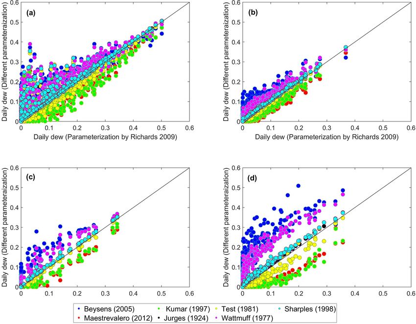
4722                        N. Atashi et al.: Delineation of dew formation zones in Iran using long-term model simulations

Figure 1. A map of Iran illustrating the geographical topography and the domain of the grid points used in the model simulation. Red stars
indicate the selected stations for uncertainty analysis.

and then divided by the time difference in seconds. The wind           early interpolated to obtain 10 s resolution). The mass and
speed at 2 m was not directly available from ERA-Interim;              heat energy balance model is written as
therefore, we obtained the wind components (U and V ) at
10 m and the surface roughness (z0 – an instantaneous fore-             dTc
                                                                            (Cc mc + Cw mw + Ci mi ) = Prad + Pcond + Pconv + Plat , (2)
cast field) and assumed a logarithmic wind profile to obtain             dt
its values at 2 m according to                                         where dTc /dt is the rate of change of the condenser temper-
                                                                     ature. Cc , Cw , and Ci are the specific heat capacity of the
         log 2+zz0
                   0   q                                               condenser, water, and ice, respectively. Here, mc , mw , and
WS =                     2 +V2 ,
                       U10                              (1)
                              10                                      mi are the mass of the condenser, water, and ice, respectively.
        log 10+zz0
                    0
                                                                       The righthand side of Eq. (2) describes the heat exchange in-
                                                                       volved in the process: Prad is the net radiation, Pcond is the
where z0 is the surface roughness and U10 and V10 are the              conductive heat exchange between the condenser surface and
horizontal wind speed components at 10 m. It is important              the ground, Pconv is the convective heat exchange, and Plat is
to understand that the logarithmic assumption is only strictly         the latent heat released by the condensation or desublimation
valid during neutral stability conditions. During stable con-          of water.
ditions (such as during nighttime) it overestimates the 2 m               The model was setup so that it assumes similar conditions
wind speed whereas in unstable conditions it underestimates            for the phase change of pre-existing water or ice on the con-
the 2 m wind speed (Riou, 1984; Holtslag, 1984; Petersen et            denser sheet. For instance, if the water on the condenser is
al., 1998; Oke, 2002; Optis et al., 2016).                             in the liquid phase (i.e., mw > 0) and the condenser temper-
                                                                       ature Tc < 0◦ , then the sheet is losing energy (i.e., the right-
2.2    Dew formation model description and output                      hand side of Eq. 2 is negative). In that case, instead of solving
                                                                       Eq. (2), Tc is assumed to be constant and the lost mass from
The global dew formation model used in this study was orig-            the liquid phase of water is transferred to the cumulated mass
inally developed by Vuollekoski et al. (2015) to estimate              of ice; i.e., the water is transformed from liquid phase to solid
dew potential. The approach is similar to Pedro and Gille-             phase. Consequently, Eq. (2) is replaced by
spie (1981) and Nikolayev et al. (1996). The model reads all                 dmw
input data (described in section 2.1) for a given grid point           Lwi       = Prad + Pconv + Plat ,                              (3)
                                                                              dt
and numerically solves the mass and heat balance equation
using a fourth-order Runge–Kutta algorithm with a 10 s time            where Lwi is the latent heat of fusion. If the water on the con-
step (i.e., the ERA-Interim data from 3 h resolution were lin-         denser is in the solid phase (i.e., mi > 0) and the condenser

Hydrol. Earth Syst. Sci., 25, 4719–4740, 2021                                            https://doi.org/10.5194/hess-25-4719-2021
N. Atashi et al.: Delineation of dew formation zones in Iran using long-term model simulations                                 4723

temperature Tc > 0◦ , a similar equation is assumed for the         densed water droplets to be eliminated on the condenser sur-
change rate of ice mass (mi ).                                      face by evaporation. Moreover, the model predicts any dew
   Note that Eq. (3) is not related to the condensation of wa-      condensation regardless of whether it is collectible or not;
ter; it only describes the phase change of the already con-         therefore, it is expected to overestimate dew yield. The spa-
densed water or ice on the condenser. For the water con-            tial data resolution is ∼ 30 km, which limits the model’s abil-
densation rate, which is assumed independent of Eq. (3), the        ity to resolve local microclimates, particularly in areas with
mass-balance equation is then assumed as                            complex topography where the topography can modify the
                                                                    large-scale winds and lead to large variations in local tem-
dm
   = max [0, Sc k (Psat (Td ) − Pc (Tc ))] ,                 (4)    peratures. However, when considering cumulative dew yield
dt                                                                  over long time periods the model performs well. Therefore,
where m represents either the mass of ice (mi ) or water (mw )      as the model uses the meteorological gridded dataset (ERA-
depending on whether Tc is below or above 0◦ . Psat (Td ) is        Interim), which is readily available for the whole globe, it
the saturation pressure at the dew point temperature and            can be applied anywhere in the world including other arid
Pc (Tc ) is the vapor pressure over the condenser sheet. Here,      and semi-arid areas even if they lack observations.
Sc is the condenser surface area and k is the mass transfer
coefficient,                                                        2.3   Cluster analysis

k = h/Lvw γ = 0.622h/Ca p,                                   (5)    Cluster analysis (CA) is an effective statistical tool and tech-
                                                                    nique that groups similar data points such that the points
where Lvw is the specific latent heat of water vaporization,        in the same group are more similar to each other than the
γ is the psychrometric constant, Ca is the specific heat ca-        points in the other groups. The group of similar data points
pacity of air, and p is the atmospheric air pressure. Here, h is    is called a cluster, which can be used for various applications
the heat transfer coefficient,                                      (Corporal-Lodangco and Leslie, 2016; Güngör and Özmen,
                                                                    2017). There are two main clustering methods: hierarchical
h = 5.9 + 4.1u(511 + 294)/ (511 + Ta ) ,                     (6)    and non-hierarchical cluster analysis. Hierarchical clustering
where u and Ta are the prevailing horizontal wind speed             (used in this study) combines cases into homogeneous clus-
and the ambient temperature 2 m above the ground. This pa-          ters where objects at one level are combined with objects
rameterization of the heat transfer coefficient is taken from       at another level and produce clusters that are not allowed
Richards (2004). However, the dew model is designed in              to overlap (Bunkers and Miller, 1996; Yim and Ramdeen,
such a manner that any functional form can be used for the          2015). Two different strategies for hierarchical clustering ex-
heat transfer coefficient, thus allowing the sensitivity of the     ist: agglomerative and divisive (Lior and Maimon, 2005).
modeled dew amounts to the formulation of the heat transfer         In this study, we used hierarchical agglomerative cluster-
coefficient to be assessed (see Sect. 3.3 for such an analysis).    ing (HAC, Nielsen, 2016), which starts with N clusters (i.e.,
   In practice, the wettability of the surface affects the va-      here, the total number of grid points) each containing one
por pressure Pc directly above it. In other words, Pc is lower      object and then joins the two objects that are most “similar”.
over a wet surface; thus, condensation may take place even if       This process continues until only one cluster containing all
Tc > Td . It is also assumed (in Eq. 4) that there is no evapora-   the data remains (Bunkers and Miller, 1996). In order to de-
tion or sublimation during daytime even if Tc > Ta . Further-       cide which clusters should be combined (for agglomerative),
more, the model simulation resets the cumulative values for         a measure of dissimilarity between sets of observations is re-
water and ice condensation at noon (local time) and takes the       quired. The similarity measurement is a critical step in hier-
preceding maximum value of mw + mi as the representative            archical clustering as it can influence the shape of the clusters
daily yield given in millimeters on a 1 m2 condenser sheet          (Nielsen, 2016). With metric data, the most commonly used
(i.e., mm m−2 d−1 equals L m−2 d−1 ).                               distance measure (a measure of the distance between pairs
   This way, the model simulation replicates the daily manual       of observations) is “Euclidean distance”. The Euclidean dis-
dew water collection of the condensed water around sunrise,         tance (dij ) between two objects i and j in a two-dimensional
i.e., after which Tc is often above the dew point temperature.      data matrix is simply the squared difference between two ob-
All terms and nomenclature are described in more detail in          servations for each of the p variables summed over the vari-
Tables 2 and 3.                                                     ables and k is the number of observations (Fovell and Fovell,
   It should be noted here that, similarly to many numerical        1993; Dokmanic et al., 2015). This can be written as
models, this model has some limitations that should be con-                v
                                                                           u p
sidered when interpreting the results. For instance, both heat      dij = t
                                                                           uX                2
                                                                                   xik − xj k .                                   (7)
and mass coefficients are semi-empirical parameters that de-                 k=1
pend on wind speed (i.e., here we used the parameterization
by Richards (2004), which is valid for u < 5 m s−1 ). In ad-        Here we applied this method to a two-dimensional matrix
dition, the 10 s time step in the model does not allow con-         (2496 × 14 610), where the number of rows represented the

https://doi.org/10.5194/hess-25-4719-2021                                          Hydrol. Earth Syst. Sci., 25, 4719–4740, 2021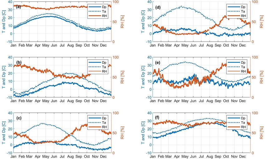
4724                        N. Atashi et al.: Delineation of dew formation zones in Iran using long-term model simulations

Table 2. Description of the dew formation model by listing the terms in Eq. (1).

       Term       Unit           Description
       dTc /dt    K s−1          Change rate of the condenser temperature
       Tc         K              Temperature of the condenser
       t          s              Time; here, the time step in the model was 10 s.
       Cc         J kg−1 K−1     Specific heat capacity of the condenser. For low-density polyethylene (LDPE) and
                                 polymethylmethacrylate (PMMA) it is 2300 J kg−1 k−1 .
       Ci         J kg−1 K−1     Specific heat capacity of ice (2110 J kg−1 k−1 )
       Cw         J kg−1 K−1     Specific heat capacity of water (4181.3 J kg−1 k−1 )
       mc         kg             Mass of the condenser given by mc = ρc Sc δc ,
                                 where ρc , Sc , and δc are the density (920 kg m−3 ), surface area (1 m2 ), and
                                 thickness of the condenser (0.39 mm).
       mi         kg             Mass of ice
       mv         kg             Mass of water, representing the cumulative mass of water
       Prad       W              Heat exchange due to incoming and outgoing radiation
                                 Prad = (1 − a)Sc Rsw + εc Sc Rlw − Pc ,
                                 where a is the condenser short-wave albedo (0.84), Sc is the condenser surface area
                                 (1 m2 ), εc is the emissivity of the condenser (0.94), and Pc is the outgoing
                                 radiative power given by the Stefan–Boltzmann law: Pc = Sc εc σ Tc4 , σ is the Stefan–Boltzmann
                                 constant (5.67 × 10⁻⁸ W m−2 K−4 ), Tc [K] is the temperature of the condenser, and Rsw and Rlw
                                 [W m−2 ] are the incoming short-wave radiation (i.e., surface solar radiation downwards) and
                                 incoming long-wave radiation (i.e., surface thermal radiation downwards).
       Pcond      W              Conductive heat exchange between the condenser surface and the ground. For simplicity, we
                                 assumed that the condenser is perfectly insulated from the ground, i.e., Pcond = 0.
       Pconv      W              Convective heat exchange
                                 Pconv = Sc (Ta − Tc )h,
                                 where Sc is the condenser surface area (1 m2 ), Ta [K] is the ambient temperature at
                                 2 m from the ground, Tc [K] is the temperature of the condenser, and h [W m−2 K−1 ] is the
                                 heat transfer coefficient that is estimated based on a semi-empirical equation (Richards, 2004)
                                 h = 5.9 + 4.1WS(511 + 294)/(511 + Ta ),
                                 where WS [m s−1 ] is the prevailing horizontal wind speed at 2 m from the ground.
       Plat       W              Latent (heat released by the condensation or desublimation of water
                                            Lvw dmdt
                                                    w   Tc > 0 ◦ C
                                 Plat =          dmi               ,
                                             Lvi dt     Tc < 0 ◦ C
                                 where Lvw [J kg−1 ] is the specific latent heat of water vaporization and Lvi [J kg−1 ] is the specific
                                 latent heat of water desublimation. Here, dmw /dt is the change rate of water whereas dmi /dt is
                                 the change rate of ice.

number of spatial grid points in the model simulation domain              ria: single linkage, complete linkage, average distance, and
and the number of columns represented the time (i.e., cumu-               Ward’s minimum variance methods, which differ in the way
lative daily dew yield).                                                  distances between entries are calculated and how the two
   After all distances were calculated, the next step is to               closest entries are defined (Stooksbury and Michaels, 1991;
merge the two closest entries to form a new cluster based                 Murtagh and Legendre, 2014). In this study, Ward’s mini-
on a linkage criterion. The linkage criterion determines the              mum variance method (Ward, 1963) is used. This method
distance between sets of observations (here, the spatial grid             is the most frequently clustering technique used in climate
points) as a function of the pairwise distances between ob-               research (Yokoi et al., 2011; Mimmack et al., 2001; Siraj-
servations. There are some commonly used linkage crite-                   Ud-Doulah and Islam, 2019) and gives the most consistent

Hydrol. Earth Syst. Sci., 25, 4719–4740, 2021                                                https://doi.org/10.5194/hess-25-4719-2021
N. Atashi et al.: Delineation of dew formation zones in Iran using long-term model simulations                                  4725

Table 3. A list of nomenclature.

                  Parameter        Unit         Description
                  α                –            Albedo of condenser sheet
                  Ca               J kg−1 K−1   Specific heat capacity of air
                  Cc               J kg−1 K−1   Specific heat capacity of the condenser
                  Ci               J kg−1 K−1   Specific heat capacity of ice
                  Cw               J kg−1 K−1   Specific heat capacity of water
                  DP               K            Dew point temperature
                  h                W K−1 m−2    Heat transfer coefficient
                  k                Per s−1      Mass transfer coefficient
                  Lvi              J kg−1       Specific latent heat of desublimation for water
                  Lvw              J kg−1       Specific latent heat of vaporization for water
                  Lwi              J kg−1       Latent heat of fusion
                  mc               kg           Mass of the condenser
                  mi               kg           Mass of ice
                  mw               kg           Mass of water
                  p                Pa           Atmospheric air pressure
                  pc               Pa           Vapor pressure over condenser
                  psat             Pa           Saturation pressure of water
                  Pcond            W            Conductive heat exchange between the condenser surface and the ground
                  Pconv            W            Convective heat exchange
                  Plat             W            Latent heat released by the condensation or desublimation of water
                  Prad             W            Heat exchange due to incoming and outgoing radiation
                  Rlw              W m2         Surface thermal radiation downwards
                  Rsw              W m2         Surface solar radiation downwards
                  Sc               m2           Surface area of condenser
                  Ta               K            Ambient temperature at 2 m
                  Tc               K            Temperature of the condenser
                  U10              m s−1        Horizontal wind speed component at 10 m
                  V10              m s−1        Horizontal wind speed component at 10 m
                  WS               m s−1        Prevailing horizontal wind speed at 2 m
                  z0               m            Surface roughness
                  δc               mm           Condenser sheet thickness
                  εc               –            Emissivity of condenser sheet
                  γ                Pa K−1       Psychrometric constant
                  σ                W m−2 k−4    Stefan–Boltzmann constant

clusters (Kalkstein et al., 1987). It calculates the means of all      By visualizing all these steps, N = 6 was found to be the
variables (the amount of dew) within each cluster, then calcu-         best number of clusters for this study because fewer clusters
lates the Euclidean distance to the cluster mean of each case,         (i.e., 3 and 4 clusters) were not able to capture the different
and finally sums across all grid points (Unal et al., 2003).           climate and dew zones. Furthermore, choosing more clusters
   In any CA, the optimal number of clusters is an important           (i.e., 7 and 10 clusters) gives some groups that replicate each
issue. There is no reliable and universally accepted method            other. The results of hierarchical clustering are usually pre-
to determine the optimal number of clusters. Kaufmann and              sented in a dendrogram (Nielsen, 2016). The dendrogram of
Weber (1996) (see also Unal et al., 2003 and Burlando, 2009)           our 6 clusters is shown in Fig. 2b.
suggested showing the total variance of subsequent merged
clusters as a function of the number of remaining clusters.
This information can be used as an indicator to decide the             3     Results
number of clusters, but a visual check of the result can still
                                                                       3.1    Spatial–temporal variation of dew occurrence and
help to make the right decision. The suitable number of clus-
                                                                              yield
ters has to be chosen somewhere in the transition between
the distance values when a sudden decrease is observed as              According to the model simulation results (cumulative daily
illustrated in Fig. 2a. In our case, few steps at N = 3, 4, 6,         dew yield in the form of dew and hoarfrost), dew formation
7, and 10 are recommended as optimal numbers of clusters.              occurred almost everywhere in Iran, as illustrated in Fig. 3,

https://doi.org/10.5194/hess-25-4719-2021                                              Hydrol. Earth Syst. Sci., 25, 4719–4740, 2021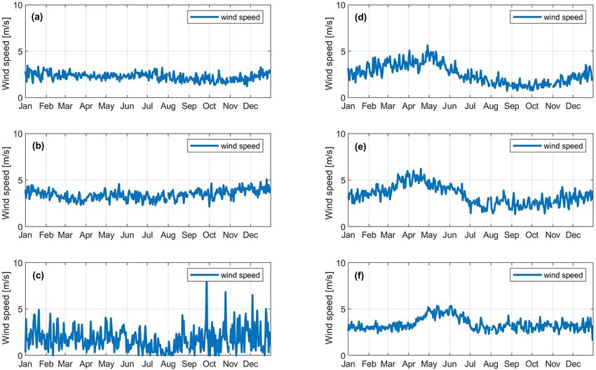
4726                        N. Atashi et al.: Delineation of dew formation zones in Iran using long-term model simulations

Figure 2. (a) Distance level at which two clusters are merged as a function of the number of clusters that result when the Ward linkage method
is applied to daily dew yield data from 1979–2018. N is the optimal number of clusters that has been chosen for this study. (b) Dendrogram
of 6 clusters.

which shows the seasonal occurrence of dew as a fraction                 yields during the summer in most parts of Iran. The monthly
of days with any dew yield. The frequency of dew occur-                  means of the cumulative dew yield are shown in Fig. S2. Both
rence was more than 80 % (∼ 75 d) in most areas of Iran in               seasonal and monthly maps show that the mountain regions
wintertime (December–February; Fig. 3a). The mean occur-                 had dew occurrence throughout the year with mean cumula-
rence of dew was rather similar during spring (March–May,                tive daily dew in the range of 0.11–0.18 L m−2 d−1 . In win-
∼ 50 d; Fig. 4b) and autumn (September–November, ∼ 40 d;                 ter, dew occurred almost everywhere in Iran with the high-
Fig. 3d) with the highest number of dew days – more than                 est yields in the southern part of the Persian Gulf and Oman
90 % (∼ 80 d) – in the mountainous and coastal areas and the             Sea coastline (mean cumulative daily dew in the range 0.15–
lowest – less than 40 % (∼ 35 d) – mostly in the dry interior            0.23 L m−2 d−1 ). In spring (i.e., April and May), a spatial
and eastern areas. The lowest frequency of dew occurrence                pattern was observed that indicated the formation of dew was
(i.e., less than 10 d) was in summer (June–August, Fig. 3c)              mainly parallel to the mountain range – Alborz (East–West)
when dew formation was limited to a narrow part along the                and Zagros (northwest and southeast). The reason could be
Caspian Sea and the northern domains of the Alborz Moun-                 related to the temperature, which increases, and relative hu-
tains.                                                                   midity, which decreases, during these spring months. There-
   Limiting the dew occurrence analysis to days with dew                 fore in spring in most areas, conditions for dew formation
yield > 0.1 L m−2 d−1 also confirmed the seasonal character-             were not present except in high elevation areas where the
istics of the temporal–spatial occurrence of dew. However,               conditions still favor dew formation. During summer and un-
in this case, the frequency of dew occurrence days was less              til the middle of autumn (i.e., July–October), a unique spatial
(in the range of 6–45 d for summer and winter, respectively;             pattern was evident that shows the distribution of dew forma-
Fig. S1 in the Supplement) and the spatial scale of dew for-             tion was limited to a narrow belt in coastal areas in the north
mation shrank to include only a few parts of the coastal and             along the Caspian Sea. In all other areas, the monthly amount
high mountain regions during spring, summer, and autumn.                 of dew yield was almost zero.
This notable difference between the two maps (i.e., Figs. 3
and S1) is associated with the model setup. The model tends              3.2     Cluster analyses – dew formation zones
to forecast any dew event, regardless of whether it can be
collectible or not. In practice, very small dew quantities are           3.2.1    Dew zones – a general overview
generally not harvestable as droplets remain pinned to the
condenser surface and gravity cannot lead them to the col-               According to our cluster analysis (CA) summarized in
lection tank.                                                            Sect. 2.2, we identified six dew formation zones in Iran
   We subsequently calculated the seasonal daily means of                (Fig. 5). The amount of daily dew yield in Iran and the re-
the cumulative dew yield (Fig. 4), which show a clear sea-               lated climatological parameters (e.g., temperature and rela-
sonal cycle with high dew yields during the winter and low               tive humidity) for dew formation as well as the percentiles
                                                                         (i.e., 25 %, median, 75 % and 99 %) of daily dew yields as av-

Hydrol. Earth Syst. Sci., 25, 4719–4740, 2021                                               https://doi.org/10.5194/hess-25-4719-2021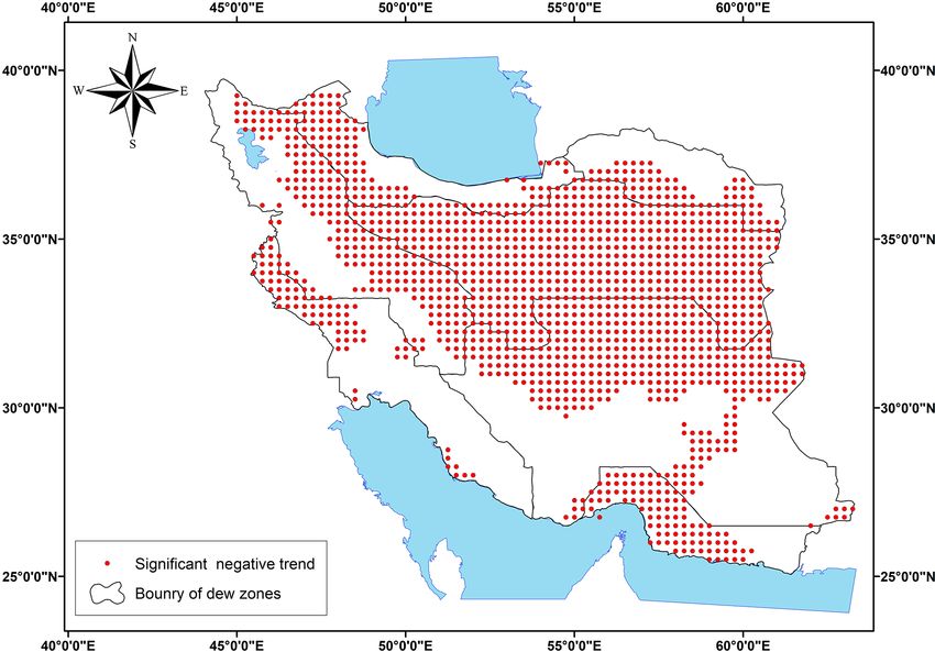
N. Atashi et al.: Delineation of dew formation zones in Iran using long-term model simulations                                  4727

Figure 3. Frequency of dew occurrence as a fraction of the days presented as an overall seasonal mean during 1979–2018. (a) Winter
(December, January, and February), (b) spring (March, April, and May), (c) summer (June, July, and August), and (d) autumn (September,
October, and November).

erages for each cluster are listed in Table 4. As will be shown      zones, and the maximum dew yield was 0.30 L m−2 d−1 (Ta-
in this section, the dew formation zones in Iran are clearly         ble 4). Interestingly, this dew zone is different compared to
aligned with topography, sources of moisture, and climate            the other dew zones concerning the annual cycle of dew for-
zones. Furthermore, the mountains and seas played major              mation; in this dew zone, dew formation occurred throughout
roles in the spatial distribution of dew formation zones. Note       the year whereas all other zones exhibit a strong annual cycle
that the maximum daily dew yield in this section is presented        (Fig. 6). The mean frequency of dew occurrence in this zone
as the 99th percentile of daily dew. In order to gain insight        was more than 330 d yr−1 . Even in summer, when dew al-
into the climatological condition in each dew zone, we se-           most vanished in other dew zones, this zone had a significant
lected one synoptic station in each dew zone and investigated        amount of dew yield (Fig. 4). The mean yearly dew yield in
some related meteorological parameters (e.g., temperature,           this region is estimated at about 53 L m−2 and the maximum
humidity, and wind speed) in the nighttime hours (i.e., 18:00,       yield is more than 100 L m−2 . The high potential of dew for-
21:00, 00:00, 03:00 LT), when dew formation occurs, for the          mation in this zone during the year is due to very suitable cli-
time period 1980–2010 (30 years), which is shown in Figs. 7          matological and geographical conditions. The synoptic sta-
and 8.                                                               tion Ramsar located in this dew zone shows the climate of
                                                                     dew zone A to be characterized by low temperature, high hu-
Dew zone A – Caspian Sea region                                      midity, and the smallest dew point depression (i.e., the small-
                                                                     est difference between the temperature and dew point) along
We identified the first dew formation zone as the “Caspian           with little variation in the relative humidity and dew point
Sea region”, which covered the southern shores of the                depression throughout the year (Fig. 7a). Moreover, due to
Caspian Sea and the northern domains of the Alborz Moun-             being a forest area, the wind speed is relatively low (Fig. 8a),
tains. This dew zone includes about 7 % of the total land area       which favors dew condensation.
of Iran (Fig. 5), which also includes the largest forest area
in Iran. The overall mean daily dew yield in this region was
∼ 0.14 L m−2 , which was the highest among all of the dew

https://doi.org/10.5194/hess-25-4719-2021                                          Hydrol. Earth Syst. Sci., 25, 4719–4740, 2021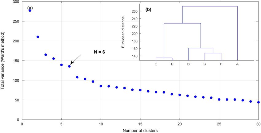
4728                       N. Atashi et al.: Delineation of dew formation zones in Iran using long-term model simulations

Figure 4. Cumulative dew yield [L m−2 d−1 ] presented as an overall seasonal mean during 1979–2018. (a) Winter (December, January, and
February), (b) spring (March, April, and May), (c) summer (June, July, and August), and (d) autumn (September, October, and November).

Figure 5. Dew formation zones based on the cluster analysis of the daily cumulative dew yield during 1979–2018.

Hydrol. Earth Syst. Sci., 25, 4719–4740, 2021                                           https://doi.org/10.5194/hess-25-4719-2021
N. Atashi et al.: Delineation of dew formation zones in Iran using long-term model simulations                                          4729

Figure 6. Long-term mean seasonal variation of the cumulative daily dew yield. Note that color coding on this figure is the same and
corresponds to the dew formation zones in Fig. 5: dew zone A (Caspian Sea; green), Zone B (Zagros region; red), Zone C (Central Iran;
orange), Zone D (Lut Desert; yellow), Persian Gulf zone (light blue), and Oman Sea zone (dark blue). The percentiles (i.e., 25 %, median,
75 % and 99 %) of the daily dew yields as averages for each cluster are presented in Table 4.

Table 4. Dew formation zones and their climate features (i.e., mean (min–max) values for meteorological parameters (T , Td , RH)) as well
as statistical analysis for overall mean daily cumulative dew yield (i.e., SD, 25, 50, 75th and 99th percentile as daily max as well as yearly
max dew yield).

                                                  Zone A          Zone B         Zone C         Zone D          Zone E         Zone F
       Tmean [◦ ]                             12 (−1–23)     12 (−1–26)        17 (3–31)      20 (7–33)      22 (9–35)    27 (16–36)
       Td mean [◦ ]                            5 (−5–14)       1 (−6–6)        1 (−5–6)       0 (−4–4)         6 (2–9)      10 (3–17)
       RHmean [%]                              69 (58–81)     52 (27–77)     40 (21–67)     30 (15–56)     37 (15–66)     39 (25–54)
       Mean dew yield ± SD [L m−2 d−1 ]       0.14 ± 0.01    0.08 ± 0.04     0.05 ± 0.05    0.03 ± 0.03    0.06 ± 0.04    0.09 ± 0.06
       25 % [L m−2 ]                                 0.08           0.04            0.02           0.01           0.03           0.03
       Median [L m−2 ]                               0.13           0.07            0.04           0.02           0.05           0.07
       75 % [L m−2 ]                                 0.19           0.11            0.06           0.04           0.08           0.13
       99 % [L m−2 ]                                 0.32           0.24            0.17           0.14            0.2           0.29
       Mean [L m−2 yr−1 ]                              53             30              18             12             24             34
       Max [L m−2 yr−1 ]                            > 100           > 60            < 50           < 45           > 70           > 80

Dew zone B – Zagros Mountains                                            all mean daily dew yield and variation in this region was
                                                                         0.08 ± 0.05 L m−2 d−1 and the highest dew yield was 0.23 L
                                                                         on a 1 m2 condenser sheet. The highest amount of dew yield
Dew zone B included the Zagros Mountains (i.e., the north-
                                                                         in this dew zone was observed during spring when the pre-
ern and central parts) and the eastern part of the Alborz
                                                                         vailing winds in this region are typically westerlies and ac-
Mountains. This dew zone covered about 15 % of Iran
                                                                         companied by moderate to high relative humidity (Fig. 7b)
(Fig. 5) and represented a mountain climate with very cold
                                                                         and low wind speed (Fig. 8b). The amount of dew yield de-
and dry weather in winter and mild weather in summer
                                                                         creased rapidly after May and was almost absent during sum-
(Fig. 7b; Zanjan station). Furthermore, due to the high el-
                                                                         mertime (Fig. 6). This is a result of higher temperature (i.e.,
evation, the diurnal variation of temperature within this
                                                                         due to atmosphere transparency and receiving high solar ra-
dew zone is large. These areas receive high levels of so-
                                                                         diation) and lower relative humidity (Fig. 7b) and also the
lar radiation during the daytime and reflect it back quickly
                                                                         lack of efficient moisture sources in this dew zone. In gen-
to space in the form of long-wave radiation during night-
                                                                         eral, the mean frequency of dew occurrence in this zone was
time. Therefore, the temperature drops rapidly during night-
                                                                         63 % (∼ 245 d). The mean yearly dew yield in this zone was
time. Enough moisture in the atmosphere, in addition to this
strong nocturnal cooling, favored dew formation. The over-

https://doi.org/10.5194/hess-25-4719-2021                                               Hydrol. Earth Syst. Sci., 25, 4719–4740, 2021
4730 N. Atashi et al.: Delineation of dew formation zones in Iran using long-term model simulations Figure 7. Nighttime (i.e., 18:00, 21:00, 00:00, 03:00 LT) long-term mean (1980–2010; 30 years) of dew point temperature (Dp ) temper- ature (Ta ), and relative humidity in six selected stations located in dew zone A–F. (a) Ramsar (dew zone A); (b) Zanjan (dew zone B); (c) Isfahan (dew zone C); (d) Tabas (dew zone D); (e) Ahvaz (dew zone E), and (f) Bandar Abbas (dew zone F). Data were obtained from the meteorological organization of Iran. Figure 8. Nighttime (i.e., 18:00, 21:00, 00:00, 03:00 LT) long-term mean (1980–2010; 30 years) of wind speed in six selected stations that are located in dew zone A–F. (a) Ramsar (dew zone A), (b) Zanjan (dew zone B), (c) Isfahan (dew zone C), (d) Tabas (dew zone D), (e) Ahvaz (dew zone E), and (f) Bandar Abbas (dew zone F). Data were obtained from the meteorological organization of Iran. Hydrol. Earth Syst. Sci., 25, 4719–4740, 2021 https://doi.org/10.5194/hess-25-4719-2021
N. Atashi et al.: Delineation of dew formation zones in Iran using long-term model simulations                               4731

about 30 L m−2 and the maximum was more than 70 L m−2              high diurnal variations in temperature, mostly a clear sky,
(Table 4).                                                         extremely sparse vegetation, and frequent high wind speed.
                                                                   In wintertime, the temperature decreases and the moisture in-
Dew zone C – Central Iran                                          creases (Fig. 7d) as a result of the westerly prevailing wind;
                                                                   thus, this dew zone experienced its highest amount of dew
The third dew zone is the Central Iran region. Central Iran        yield in winter. In contrast, in the warm season (i.e., May–
consists of the southern slopes of the Alborz Mountains in         September) dew was almost completely absent (Fig. 6). The
the north, the Zagros Mountains in the south, and the cen-         reason is due to high temperature, longer daytime duration,
tral Iranian ranges. These areas are mostly hot and very dry.      and a strong north–south pressure gradient between the ther-
The Alborz and Zagros mountains prevent moisture penetra-          mal low-pressure system over the desert lands and a cold
tion from the Caspian Sea and westerlies so that the amount        high-pressure over the Hindu Kush in northern Afghanistan
of water vapor pressure is very low (∼ 7 hPa; Masoudian,           (Alizadeh-choobari et al., 2014) that generates the strong
2011). This zone covered about 20 % of Iran and included the       summer wind called “the Sistan wind of 120 d”. It has this
Kavir Desert basin, Salt Lake, and some parts in the north-        name because it occurs during late May through late Septem-
east (Fig. 5). The overall mean daily dew yield in this re-        ber (about 4 months) in the east and southeast of the Iranian
gion is estimated to be about 0.05 L m−2 and the maximum           Plateau, particularly the Sistan Basin. The typical wind speed
yield (99th percentile) was about 0.21 L m−2 d−1 . The aver-       of the Sistan is 30–40 km h−1 , but it could occasionally ex-
age yearly dew yield in this region was about 18 L m−2 and         ceed 100–110 km h−1 , which impedes dew formation during
the maximum yield was less than 50 L m−2 yr−1 . The dew            the summer season. Thus, the key factors for dew condensa-
period in this zone starts in autumn and continues until mid-      tion (high humidity and low wind speeds) are not present for
spring (i.e., October–April); however, the frequency of dew        most of the year in this dew zone. Consequently, the average
occurrence (> 0.1 L m−2 d−1 ) is about 80 d. Isfahan station       yearly dew yield in this zone was low – about 12 L m−2 – and
is located in this dew zone and is representative of the cli-      the maximum yield was about 40 L m−2 yr−1 .
mate of this dew zone. The dew point temperatures are very
low (mainly around or less than zero) all year round and have      Dew zone E – Persian Gulf region
slight annual variation (Fig. 7c). The relative humidity is low
in spring but increases in Autumn (Fig. 7c) when tempera-          The Persian Gulf dew zone included the coastal line of
tures start to decrease and dew formation also starts. Further-    the Persian Gulf and some parts of the western half of the
more, the wind speed is quite weak (less than 2.5 m s−1 on         land areas in Iran (∼ 9 % of all grid points; Fig. 5). The
average, Fig. 8c) and does not have a pronounced annual cy-        overall mean daily dew yield is about 0.06 L m−2 , which is
cle. Therefore, humidity and temperature are most likely the       lower than the other coastal zones in the north (i.e., Caspian
key factor in formation of dew in this station. More specif-       Sea; dew zone A) and south of Iran (i.e., Oman Sea; dew
ically, once relative humidity starts increasing and tempera-      zone F). However, the maximum daily dew yield in win-
ture decreases (in autumn and winter), dew can also form.          ter (i.e., December–February) was higher than that in the
                                                                   Caspian Sea zone. Indeed, this dew zone benefits from two
Dew zone D – Lut Desert                                            huge sources of moisture (i.e., the Persian Gulf and Karun
                                                                   river), although high temperatures (e.g., as observed at the
We identified the fourth dew zone (i.e., Dew zone D) that          synoptic station Ahvaz; Fig. 7e), thermal high pressure, and
included the Lut Desert (175 000 km2 ; Alizadeh-choobari et        dry winds, especially during the warm season (i.e., May–
al., 2014), which is an arid and hyper-arid desert (Fig. 5).       September), do not favor the formation of dew. Therefore, the
This zone, with 35 % of all grid points in the land areas of       period of dew formation was about 7 months starting in Oc-
Iran, is the largest dew zone; however, it has the least dew oc-   tober and ending in April. However, the frequency of dew oc-
currence (∼ 15 d yr−1 with dew yield > 0.1 L m−2 d−1 ) and         currence > 0.1 L m−2 d−1 is about 117 d during November–
a mean yield of 0.03 L m−2 d−1 . Indeed, this part of the          February (Fig. 6) when relative humidity is at its highest level
country includes the driest areas (i.e., water vapor pressure      and temperature and wind speed are relatively low compare
is < 5 hPa). Based on a survey conducted by scientists at          to the rest of the year (Figs. 7e and 8e). The average yearly
NASA’s Earth Observatory during the summer of 2003–                dew yield in this zone was about 24 L m−2 and the maximum
2009 (see Temperature of Earth: https://www.universetoday.         was > 70 L m−2 yr−1 (Table 4).
com/14367/planet-earth, last access: 7 August 2021), the Lut
Desert was the hottest (∼ 71◦ ) land surface on Earth (see also    Dew zone F – Oman Sea region
Khandan et al. (2018)). The synoptic station Tabas is located
in this dew zone and has a climate characterized by high tem-      The coastline along the Oman Sea and the Strait of Hor-
peratures (higher than the synoptic stations we considered in      muz formed the sixth dew zone, which is also the small-
dew zones A, B, and C) and low relative humidity in sum-           est dew zone in Iran covering only 5 % of the grid points
mer (Fig. 7d). In addition to the dryness, these areas have        (Fig. 5). The overall mean daily dew yield in this zone was

https://doi.org/10.5194/hess-25-4719-2021                                       Hydrol. Earth Syst. Sci., 25, 4719–4740, 2021
4732 N. Atashi et al.: Delineation of dew formation zones in Iran using long-term model simulations Figure 9. Mann–Kendall trend test on mean yearly dew yield over the years 1979–2018 as predicted by Sen’s slope estimator. Only locations with a statistically significant trend (p < 0.05) are shown. Red points present locations with a negative trend regardless of their decreased values, and the white parts did not show any significant trend at (p < 0.05). about 0.09 L m−2 and the maximum dew yield was about dewy days (∼ 150 d) in this zone is lower than in dew zone A 0.23 L m−2 d−1 (Table 4), which was the highest among all (the Caspian Sea region; Fig. 7). dew zones. This is not surprising because this region benefits from a generous source of moisture (i.e., the Oman Sea, Per- 3.2.2 Long-term temporal variation in dew formation sian Gulf, Arabian Sea, and Indian Ocean through the sum- zones mer monsoon). Observations from the station Bandar Ab- bas confirm the presence of a moisture source, as the dif- In order to investigate the long-term (1979–2018) variation ference between the temperature and dew point temperature of dew formation, we applied the Mann–Kendall trend test is quite small (about 5◦ ) and constant throughout the year. (Pohlert, 2016) to the yearly means of dew yield with a con- However, despite these conditions, the formation of dew was fidence level of 95 %. Figure 9 shows the statistical signifi- mostly limited to the cold season (i.e., starting in Septem- cance (p < 0.05) of the overall changes in the mean yearly ber and ending by March; Fig. 6); during the warm sea- dew yield. The result of this trend analysis showed that in son (i.e., April–August), dew occurrence was rare (Fig. 6). more than 60 % of the land areas in Iran (i.e., mostly dew The reason is likely due to the increase in wind speed (as zones C and F and the northern half of dew zones B and D), shown by observations at the synoptic station Bandar Abbas; dew formation has decreased during the past 40 years. The Fig. 8e) and the temperature during summer. In particular, in remaining parts of Iran did not show any significant trend the warm season, high temperatures lead to the formation of (α = 5 %); however, their negative slope (82 % of the re- low-pressure systems (i.e., the Gang low pressure system and mained grid points) might be a sign of a future decrease in Persian Gulf low pressure system) over the seas, which inten- dew formation for these regions. Such negative trends in dew sified the hot and humid conditions in the southern coastal yield over a wide geographical region could be due to differ- region. High humidity results in amplified long-wave radia- ent reasons that control the condensation process. To iden- tion downwards and therefore less radiative cooling. In ad- tify potential causes for the detected decrease in dew forma- dition, due to the strong gradient between the low pressure tion, we first calculate correlations between the dew forma- over the Persian Gulf and the high pressure over Saudi Ara- tion and meteorological parameters (temperature, dew point bia, an intense airflow is stimulated such that condensation temperature, dew point depression, relative humidity, wind does not occur despite high humidity. Lastly, although this speed, and cloud cover obtained from ERA-Interim) for each zone had the highest daily dew yield, it does not have the dew formation zone (Table 5). Subsequently, we calculate the highest yearly yield (i.e., > 80 L m−2 ) since the frequency of trend for each of the six meteorological variables. Hydrol. Earth Syst. Sci., 25, 4719–4740, 2021 https://doi.org/10.5194/hess-25-4719-2021
N. Atashi et al.: Delineation of dew formation zones in Iran using long-term model simulations                                                      4733

Table 5. Correlation between long-term mean daily dew yield and meteorological parameters obtained from ERA-Interim for the time
period 1979–2018 and Sen’s trend slope in the meteorological variables per decade (i.e., 10 years).

                          Zone                                     T             Td      T − Td             RH        WS      Cloud
                                                                  [◦ ]           [◦ ]       [◦ ]            [%]   [m s−1 ]    cover
                                                                                                                                [%]
                          Zone A         Correlation            0.25           0.28       −0.15        −0.18       −0.62     −0.24
                                         Trend slope            0.6∗            0.1        0.4∗        −1.6∗       0.02∗     −0.01
                          Zone B         Correlation         −0.93          −0.75         −0.97            0.95    −0.67       0.93
                                         Trend slope          0.6∗          −0.09          0.6∗            −2∗     0.02∗     −0.01∗
                          Zone C         Correlation         −0.96          −0.88         −0.96         0.98       −0.75       0.84
                                         Trend slope          0.7∗           −0.4            1∗        −2.5∗      −0.04∗     −0.01∗
                          Zone D         Correlation         −0.94         −0.74          −0.95            0.98    −0.37       0.74
                                         Trend slope          0.4∗        −0.04∗           0.4∗            −0.8   −0.001          0
                          Zone E         Correlation         −0.95          −0.69         −0.94         0.97       −0.67       0.84
                                         Trend slope          0.3∗           0.4∗          0.01        −0.4∗       0.05∗          0
                          Zone F         Correlation         −0.95          −0.75         −0.94            0.88    −0.53       0.42
                                         Trend slope          0.3∗           0.4∗          −0.1             0.1    0.02∗          0
                        ∗ Values with an asterisk indicate a statistically significant trend (p < 0.05).

   The correlation analysis (i.e., Pearson’s correlation) re-                           largely explain the decreasing trend in dew yield during the
vealed that dew formation in almost all dew zones (i.e., B–                             last 4 decades (1979–2018).
F) has a very strong negative correlation (values of −0.93
to −0.95) with temperature, a strong positive correlation with                          3.3     Uncertainties in the dew model simulation results
relative humidity (values of 0.88 to 0.98), and a negative cor-
relation with the dew point depression (−0.69 to −0.88). In                             A detailed investigation of the model setup, i.e., input param-
contrast, dew zone A (the Caspian Sea) has weak correla-                                eters (e.g., emissivity and albedo), wind profile assumptions,
tions between dew formation and temperature, relative hu-                               and heat transfer assumptions, revealed that the dew yield
midity, and dew point temperature indicating dew formation                              estimation is very sensitive to the heat transfer coefficient.
in this region is controlled by different processes. In addition,                       In order to obtain an estimation of the final uncertainties in
zone A is the only zone to have a weak and negative corre-                              the model simulation results (i.e., daily dew yield) caused by
lation between dew formation and cloud cover. These huge                                the heat transfer coefficient, we ran the model with eight dif-
differences between dew zone A and other zones are likely                               ferent parameterizations of the heat transfer coefficients for
due to differences in topography as dew zone A is mainly                                four grid points (Table 6) for one year (2000). We selected
covered by forests and the behavior of some climatological                              four stations or grid points (red stars in Fig. 1) in different
variables can be different than the rest of the areas. A mod-                           dew zones: Ramsar station in dew zone A, Zanjan in dew
erate negative correlation between dew formation and wind                               zone B, Tabas in dew zone D, and Bandar Abbas in dew
speed (−0.62) does exist in zone A, which may indicate that                             zone F.
wind speed is the meteorological parameter with the most                                   Figure 10 shows the daily dew yields estimated using the
influence on dew formation in Zone A.                                                   parameterization by Richards (2004, this study) against the
   When the long-term trends are considered, air tempera-                               daily dew yields obtained from the seven other parameter-
ture, which has a negative effect on dew formation, showed                              izations listed in Table 6. For all four grid points consid-
a significant positive trend (p < 0.05) in all dew zones over                           ered, the parameterizations of Beysens et al. (2005) and Wat-
the 40 years. The magnitude of these changes for zones A–                               muff et al. (1997) give the largest estimates of daily dew
F was 0.6, 0.6, 0.7, 0.4, 0.3, and 0.3◦ per decade, respec-                             yields whereas the parameterizations of Kumar et al. (1997)
tively. Relative humidity (RH) and cloudiness had a posi-                               and Maestre-Valero et al. (2011) give the lowest estimates
tive effect on dew formation (except in Zone A); however,                               (Fig. 10, Table 6). Figure 10 also demonstrates that the
they both had a negative trend over 40 years. The average                               largest differences occur for the very low values of daily dew
decrease in relative humidity for the dew zones (i.e., A–E)                             yield.
was about 1.5 % per decade (Table 5). Therefore, the in-                                   The absolute differences in daily dew yields between the
crease in temperature and decrease in RH and cloudiness can                             parameterizations are calculated in Table 6. At Ramsar (lo-
                                                                                        cated in dew zone A in a forested region), the daily mean dew

https://doi.org/10.5194/hess-25-4719-2021                                                                   Hydrol. Earth Syst. Sci., 25, 4719–4740, 2021
You can also read