Suitability of fibre-optic distributed temperature sensing for revealing mixing processes and higher-order moments at the forest-air interface
←
→
Page content transcription
If your browser does not render page correctly, please read the page content below
Atmos. Meas. Tech., 14, 2409–2427, 2021
https://doi.org/10.5194/amt-14-2409-2021
© Author(s) 2021. This work is distributed under
the Creative Commons Attribution 4.0 License.

Suitability of fibre-optic distributed temperature sensing for
revealing mixing processes and higher-order moments at
the forest–air interface
Olli Peltola1 , Karl Lapo2,3 , Ilkka Martinkauppi4 , Ewan O’Connor1,5 , Christoph K. Thomas2,3 , and Timo Vesala6,7
1 Climate   Research Programme, Finnish Meteorological Institute, P.O. Box 503, 00101 Helsinki, Finland
2 Micrometeorology    Group, University of Bayreuth, Bayreuth, Germany
3 Bayreuth Center for Ecology and Environmental Research, BayCEER, University of Bayreuth, Bayreuth, Germany
4 Geological Survey of Finland, Kokkola, Finland
5 Department of Meteorology, University of Reading, Reading, UK
6 Institute for Atmosphere and Earth System Research/Physics, Faculty of Science, University of Helsinki,

P.O. Box 68, 00014 Helsinki, Finland
7 Institute for Atmospheric and Earth System Research/Forest Sciences, Faculty of Agriculture and Forestry,

University of Helsinki, P.O. Box 27, 00014, Helsinki, Finland

Correspondence: Olli Peltola (olli.peltola@fmi.fi)

Received: 27 June 2020 – Discussion started: 23 September 2020
Revised: 26 January 2021 – Accepted: 15 February 2021 – Published: 26 March 2021

Abstract. The suitability of a fibre-optic distributed tem-       component which was, however, quantified, and its effect on
perature sensing (DTS) technique for observing atmospheric        turbulence statistics was accounted for. Underestimation of
mixing profiles within and above a forest was quantified, and     air temperature fluctuations at high frequencies caused 20 %–
these profiles were analysed. The spatially continuous obser-     30 % underestimation of temperature variance at typical flow
vations were made at a 125 m tall mast in a boreal pine forest.   conditions. Despite these limitations, the DTS measurements
Airflows near forest canopies diverge from typical bound-         should prove useful also in other studies concentrating on
ary layer flows due to the influence of roughness elements        flows near roughness elements and/or non-stationary periods,
(i.e. trees) on the flow. Ideally, these complex flows should     since the measurements revealed spatio-temporal patterns of
be studied with spatially continuous measurements, yet such       the flow which were not possible to be discerned from single
measurements are not feasible with conventional micromete-        point measurements fixed in space.
orological measurements with, for example, sonic anemome-
ters. Hence, the suitability of DTS measurements for study-
ing canopy flows was assessed.
   The DTS measurements were able to discern continuous           1   Introduction
profiles of turbulent fluctuations and mean values of air tem-
perature along the mast, providing information about mix-         The majority of the interaction between the atmosphere and
ing processes (e.g. canopy eddies and evolution of inversion      Earth’s surface takes place in a shallow air layer termed the
layers at night) and up to third-order turbulence statistics      atmospheric boundary layer (ABL). Insights on the atmo-
across the forest–atmosphere interface. Turbulence measure-       spheric mixing processes in this layer are required in or-
ments with 3D sonic anemometers and Doppler lidar at the          der to gain a better understanding on ecosystem–atmosphere
site were also utilised in this analysis. The continuous pro-     feedbacks, air quality and weather-forecasting-related issues.
files for turbulence statistics were in line with prior studies   Studies near the surface typically rely on time series analy-
made at wind tunnels and large eddy simulations for canopy        sis, since spatial details of the mixing close to the ground
flows. The DTS measurements contained a significant noise         are difficult to measure with conventional instrumentation.

Published by Copernicus Publications on behalf of the European Geosciences Union.
2410                                                                                              O. Peltola et al.: DTS in forest

However, similarity theories underlying the analysis of ob-         balloons or unoccupied aerial vehicles (UAVs) (Poulos et al.,
servations and models are posed in length scales, calling for       2002; Frehlich et al., 2008; Higgins et al., 2018; Egerer et al.,
spatially explicit sampling. In addition, turbulence statistics     2019), may partly fill the gap, yet, with these techniques, only
or spatial details of different flow structures are typically de-   non-continuous campaign type measurements are possible,
rived from a time series of observations by assuming ergodic        resulting in low temporal coverage and representativeness.
hypothesis or Taylor’s frozen turbulence hypothesis (Taylor,        Furthermore, measurements close to or in-between rough-
1938). Yet, it has been recognised that these hypotheses are        ness elements (trees and buildings) are typically not possible
not universally valid (Mahrt et al., 2009; Thomas, 2011; Hig-       with these mobile platforms.
gins et al., 2012, 2013; Cheng et al., 2017).                          Distributed temperature sensing (DTS) has been utilised in
   Atmospheric boundary layer flows feature other flow              environmental research since the first studies of Selker et al.
modes besides turbulence, and these flow modes exhibit spa-         (2006) and Tyler et al. (2009). The measurement method pro-
tial patterns which are not directly related to their tempo-        vides spatially continuous profiles along a fibre-optic cable
ral counterparts. For instance, transient submesoscale mo-          which can be freely distributed in the measurement domain.
tions may occur in the weak-wind stable boundary layer              The DTS data are provided at a similar temporal and spa-
(Mahrt, 2014), which can travel in the opposite direction of        tial resolution along the cable to that of conventional in situ
the mean flow (Zeeman et al., 2015) and interact with turbu-        measurements, lending direct comparison between the mea-
lence (Kang et al., 2015; Sun et al., 2015; Mahrt and Thomas,       surement techniques and complementary analyses of joint
2016; Vercauteren et al., 2016), inflicting intermittent mixing     measurements with multiple techniques. The measurement
and transport of gases, heat and momentum. Mechanistic un-          technique relies on optical time domain reflectometry and
derstanding of these non-turbulent motions and related pro-         measurement of Raman backscattering of a light pulse travel-
cesses are limited, partly due to the missing spatial informa-      ling in the fibre-optic cable (Dakin et al., 1985; Selker et al.,
tion on the flow.                                                   2006). Due to its ability to provide spatio-temporal informa-
   Besides submeso motions in stable conditions, the flow in        tion at scales (down to 1 s and 25 cm) that are commensurate
the roughness sublayer (RSL), by definition, exhibits spatial       with the scales prevalent near the surface, the measurement
patterns that call for spatial sampling. For instance, flows        method shows promise in answering many persistent, unan-
within and above forest canopies are dominated by large             swered questions related to near-surface flow.
coherent structures (Finnigan, 2000; Thomas and Foken,                 A growing body of research has already utilised DTS
2007a, b; Thomas et al., 2008; Finnigan et al., 2009) that          measurements in atmospheric studies (Keller et al., 2011;
are in continuous interaction with the surface roughness el-        Thomas et al., 2012; Euser et al., 2014; de Jong et al., 2015;
ements; this interaction can cause persistent spatial variabil-     Sayde et al., 2015; Zeeman et al., 2015; Pfister et al., 2017;
ity in the flow and turbulent transport (Bohrer et al., 2009;       Higgins et al., 2018; Schilperoort et al., 2018; Higgins et al.,
Schlegel et al., 2015) raising questions about the experi-          2019; Izett et al., 2019; Mahrt et al., 2019; Pfister et al.,
mental approach deployed in global measurement networks             2019). The bulk of the studies have concentrated on noc-
monitoring the turbulent transport of gases above ecosystems        turnal flows near the surface (Keller et al., 2011; Thomas
(Baldocchi, 2014). Surface spatial heterogeneities also dom-        et al., 2012; Zeeman et al., 2015; Pfister et al., 2017; Izett
inate the flow properties in the urban RSL, with urban sur-         et al., 2019; Mahrt et al., 2019; Pfister et al., 2019), and a
faces exhibiting large variability in the surface heat flux and,    few have concentrated on transition periods (Higgins et al.,
hence, the thermal production of turbulence (Barlow, 2014).         2018, 2019). By utilising different DTS measurement con-
In general, the analysis of the effect of abrupt edges, or ir-      figurations, some studies have done distributed wind speed
regular discontinuities in surface characteristics, on the flow     (heated cables) (Sayde et al., 2015; Pfister et al., 2017) or
requires spatially explicit sampling.                               humidity (wetted cables) measurements (Euser et al., 2014;
   Remote sensing instrumentation is capable of resolving           Schilperoort et al., 2018), whereas others have examined
the spatial detail of the flow (e.g. Newsom et al., 2008;           the radiation error of the cables (de Jong et al., 2015; Sig-
Träumner et al., 2012); yet, small-scale features close to the      mund et al., 2017). However, thorough and critical analysis
ground are typically missing, and measurements near ob-             on the feasibility of DTS systems for measuring atmospheric
stacles such as trees and buildings are not feasible. On the        scalar mixing has not been done since the pioneering study of
other hand, conventional precise in situ measurements cir-          Thomas et al. (2012). We complement the analysis made by
cumvent these limitations but are fixed in space (e.g. at mea-      Thomas et al. (2012) by comparing the DTS measurements
surement towers). Consequently, spatial details of the flow         against conventional in situ analysers within and above an
can be deduced only by assuming Taylor’s frozen turbu-              aerodynamically rough forest canopy from the ground up to
lence hypothesis. Hence, there is an evident observational          120 m above the ground. Furthermore, we evaluate whether
gap between the conventional measurement techniques (re-            third-order statistics could be discerned from the DTS data to
mote sensing vs. in situ), which results in limited under-          reveal important transport process information of the sweep
standing of flow processes falling in this observational gap.       ejection cycles created by the coherent structures. Devia-
In situ measurements on moving platforms, such as tethered          tions from Gaussian distribution are typically related to large

Atmos. Meas. Tech., 14, 2409–2427, 2021                                              https://doi.org/10.5194/amt-14-2409-2021
O. Peltola et al.: DTS in forest                                                                                           2411

coherent eddies or submeso air motions, whereas isotropic        low the ICOS EC measurement level was measured follow-
turbulence follows Gaussian distribution more closely, and       ing ICOS procedures (Montagnani et al., 2018). Radiation-
hence, higher-order statistics are needed for studying these     shielded and ventilated platinum wire thermistors (PT100)
more organised flow patterns. We also assess the random un-      were located at 3.3, 5.8, 8.8, 12.5, 16.8, 21.6 and 27 m heights
certainties in the DTS measurements and their effect on the      above the ground. These measurements provide suitable data
derived statistics. Finally, we demonstrate how a combina-       for comparison against the temperature data measured with
tion of vertical DTS measurements, together with 3D sonic        DTS. Radiation components were measured with a four-
anemometers and upward pointing Doppler lidar measure-           component net radiometer (model CNR4; Kipp & Zonen,
ments, can be used to obtain continuous turbulence profiles,     Delft, the Netherlands) mounted on the mast at 67 m height.
starting from the canopy sublayer all the way up to boundary        Besides conventional in situ measurements on the mast,
layer top. Consequently, the DTS system bridges the scales       the atmospheric boundary layer was profiled with a scanning
between individual in situ measurement devices and remote        Doppler wind lidar (HALO Photonics StreamLine; Pearson
sensing with lidar.                                              et al., 2009) located on the roof of a building approximately
                                                                 400 m southwest from the mast. The wind lidar operates at
                                                                 1.5 µm wavelength and, when pointing vertically, is config-
2     Materials and methods                                      ured to provide a profile of radial velocities approximately
                                                                 every 14 s with 30 m spatial resolution at Hyytiälä (Hirsikko
2.1    Measurement site and instrumentation                      et al., 2014). The Doppler lidar provides data from 75 to
                                                                 9585 m distance, and the clearest signal typically originates
The measurement campaign took place from 3 June to               from the boundary layer where the aerosol loading is the
8 July 2019 at the Hyytiälä SMEAR II (Station for Measur-        highest.
ing Forest Ecosystem–Atmosphere Relations) station (Hari
and Kulmala, 2005) located in central Finland (61.845◦ N,        DTS measurement setup
24.289◦ E). The station is a member of several measure-
ment networks, including ICOS (Integrated Carbon Observ-         The DTS instrument (ULTIMA-S, 5 km variant; Silixa Ltd,
ing System; Franz et al., 2018) and ACTRIS (Aerosols,            Hertfordshire, UK) was housed in a wooden cabin located
Clouds, and Trace gases Research Infrastructure), and thus,      approximately 30 m away from the measurement mast. A
a wide range of atmospheric and biospheric measurements          total of two 50 L calibration baths were filled with wa-
is conducted continuously. The site is dominated by a Scots      ter, equipped with reference thermometers (PT100; sup-
pine (Pinus Sylvestris) stand, with an average tree height (h)   plied with the DTS instrument and logged with the DTS
of approximately 17 m, resulting in zero-plane displacement      instrument at 0.01 ◦ C precision), and the fibre-optic cable
height (d) of 14 m. The forest canopy is between 10 and          was guided twice through both baths. The baths were also
17 m, and the all-sided leaf area index (LAI) was approxi-       equipped with aquarium pumps to ensure continuous mix-
mately 8 m2 m−2 in 2015. Below 10 m height, there is rela-       ing and prevent stratification of the water. Water temperature
tively open trunk space. The terrain is undulating, with the     in the baths was controlled with two thermostats (RC 6 CS,
main slope (2◦ ) directed roughly in north–south direction.      Lauda Dr. R. Wobser GmbH & Co. KG, Domicile Lauda–
More details on the in-canopy turbulence and canopy struc-       Königshofen, Germany) and the bath temperatures were set
ture are given in Launiainen et al. (2007) and on the terrain    at 5 and 30 ◦ C so that the temperatures bracketed the am-
undulation in Alekseychik et al. (2013).                         bient air temperatures during the campaign. The baths were
   The measurements utilised in this study were conducted on     located next to the wooden cabin which housed the DTS in-
the SMEAR II station’s 125 m tall main mast. There are 3D        strument.
ultrasonic anemometers installed at five heights on the mast        The measurements were conducted in double-ended mode,
(5.5, 24.6, 27, 68.3 and 125 m above ground), providing tur-     with signals from both directions stored separately (see
bulent fluctuations of temperature and three wind speed com-     Sect. 2.2 for processing). The path of the fibre-optic cable
ponents at 10 Hz sampling frequency. Different anemome-          began by running through both calibration baths, then up and
ters are present at different heights (USA-1, manufactured by    down the 125 m tall mast, and returning through the calibra-
METEK Meteorologische Messtechnik GmbH, Germany, at              tion baths again to finish. The cable was fastened to approxi-
5.5, 68.3 and 125 m; Solent Research model 1012R2 by Gill        mately 0.5 m long horizontal booms located every 5 to 10 m
Instruments Limited, UK, at 24.6 m; HS-50 by Gill Instru-        along the mast by squeezing the cable gently between two
ments Limited, UK, at 27 m). The anemometer at 27 m height       metallic plates covered with rubber slabs and soft electrical
is part of the eddy covariance (EC) flux measurement setup       tape. Despite careful mounting of the cable, the cable holders
for ICOS measurements (Rebmann et al., 2018). Measure-           caused disturbances in the data, and consequently, data points
ments at 5.5 m height started on 18 June 2019; all other 3D      close to the holders were removed from subsequent analysis.
sonic anemometers were measuring continuously through-           Horizontal separation between the cable and the 3D sonic
out the study period. The air temperature vertical profile be-   anemometers was 3.5 m at all levels. The vertical DTS mea-

https://doi.org/10.5194/amt-14-2409-2021                                           Atmos. Meas. Tech., 14, 2409–2427, 2021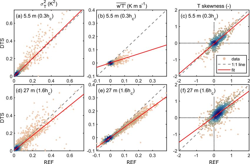
2412                                                                                                       O. Peltola et al.: DTS in forest

surements extended from 2 to 120 m above the ground. This        where u∗ is friction velocity. T∗ was calculated using data
setup enabled reference measurements at both the beginning       from the 3D sonic anemometer at 27 m height throughout the
and end of the cable from the calibration baths and provided     study.
a double measurement of the DTS vertical air temperature            DTS measurements were post-field calibrated using the
profile at 12.7 cm spatial and 1 Hz temporal resolution. Note,   measurements in the calibration baths and the following
however, that, in double-ended mode, each direction along        equation (e.g. van de Giesen et al., 2012):
the cable is measured sequentially, so that the temperature
data were available at 0.5 Hz resolution. A white, thin (outer                                             γ
                                                                 T (x, t) =                                     Rx             ,      (4)
                                                                                       Ps (x,t)                         0    0
diameter 0.9 mm) aramid-reinforced 50 µm multimode fibre-                     ln       Pas (x,t)       + C(t) +   0 1α(x )dx
optic cable (AFL Telecommunications LLC, Duncan, SC
29334, US) was utilised in this study in order to minimise       where T is the calibrated temperature as a function of po-
the impact of solar heating on the measurements (de Jong         sition along the fibre (x) and time (t), γ is a DTS system-
et al., 2015; Sigmund et al., 2017) and to maximise the high-    specific constant, Ps and Pas are the measured Stokes and
frequency response of the setup.                                 anti-Stokes signals, C is a time-dependent calibration pa-
                                                                 rameter, and the integral in the denominator is related to the
2.2    Data processing                                           differential attenuation of the anti-Stokes and Stokes signals
                                                                 along the cable. The double-ended configuration allowed the
All high-frequency time series (3D sonic anemometers and         determination of the differential attenuation at each location
DTS) were separated into the slowly varying mean and fluc-       along the cable separately, which was calculated following
tuations around the mean as follows:                             van de Giesen et al. (2012) separately for each 30 min averag-
                                                                 ing period. However, measurements from only one direction
T = T0 +T,                                                 (1)
                                                                 were utilised to calculate the temperature along the cable,
                                                                 i.e. measurements from the two directions were not averaged.
where T is the measured high-frequency time series, overbar
                                                                 After determining the differential attenuation, the calibration
denotes averaging in time, and prime (0 ) fluctuations around
                                                                 parameters γ and C were first determined by fitting Eq. (4)
the mean are calculated as a residual (T 0 = T − T ). Process-
                                                                 to the reference measurements made in the calibration baths
ing of 3D sonic anemometer data followed commonly ap-
                                                                 for each time step separately producing time series for both
plied procedures. The data were despiked in order to remove
                                                                 parameters. Then, during the second processing stage, the
spurious outliers from the time series (Mauder et al., 2013),
                                                                 data were calibrated again by fixing the value of γ to 476 K
and the wind vectors were aligned with the long-term mean
                                                                 (mean of values obtained during the first processing stage)
wind field following the planar fit coordinate rotation method
                                                                 and letting C vary between time steps. We opted to process
(Wilczak et al., 2001). Turbulent fluxes and statistics (vari-
                                                                 the data with this three-step procedure since (1) it resulted in
ance and skewness) were calculated with 30 min resolution
                                                                 less noisy calibration parameters, (2) theoretically γ should
throughout this study, unless otherwise noted. Note that, as
                                                                 be constant and (3) a reduction in fit parameters is desirable
H2 O fluctuations were not measured at most heights, it was
                                                                 given the number of calibration baths. The calibration param-
not possible to convert the sonic temperature to actual tem-
                                                                 eter C showed only a slight variation in time (1.460 ± 0.003,
perature (Schotanus et al., 1983; Foken et al., 2012). This
                                                                 mean ± SD), which resulted from a parabolic dependence on
caused a slight H2 O variance and H2 O flux-dependent bias
                                                                 the indoor temperature of the cabin housing the DTS instru-
in temperature variance and w0 T 0 covariance, respectively.
                                                                 ment. After quality filtering, 1513 (89 % of the whole period)
The stability of the atmospheric surface layer was evaluated
                                                                 30 min periods of DTS data were available for further analy-
based on the stability parameter as follows:
                                                                 sis.
      z−d                                                           The high-frequency response of the DTS system was eval-
ζ=        ,                                                (2)   uated by transforming the temperature time series to fre-
       L
                                                                 quency domain with Fourier transform and comparing the
where z denotes height, d is displacement height, and L is       power spectra against reference power spectra measured with
Obukhov length. Negative values for ζ denote unstable strat-     the sonic anemometers. Following EC data-processing pro-
ification (buoyancy increases turbulence), positive values de-   cedures (e.g. Ibrom et al., 2007), the noise in the power spec-
note stable stratification (buoyancy diminishes turbulence)      tra was subtracted from the signal prior to the comparison.
and zero denotes neutral stratification. A scaling parameter     By assuming that the DTS system as a whole behaves as a
for temperature was used to describe the temperature vari-       first-order response sensor, then, after normalisation, the ra-
ability in the atmospheric surface layer and was defined as      tio between the power spectra from DTS and the reference
follows:                                                         can be approximated by the following:

       w0 T 0                                                                            1
T∗ =          ,                                            (3)   TH (f ) =                             ,                                (5)
        u∗                                                                    1 + (2πf τ )2

Atmos. Meas. Tech., 14, 2409–2427, 2021                                                   https://doi.org/10.5194/amt-14-2409-2021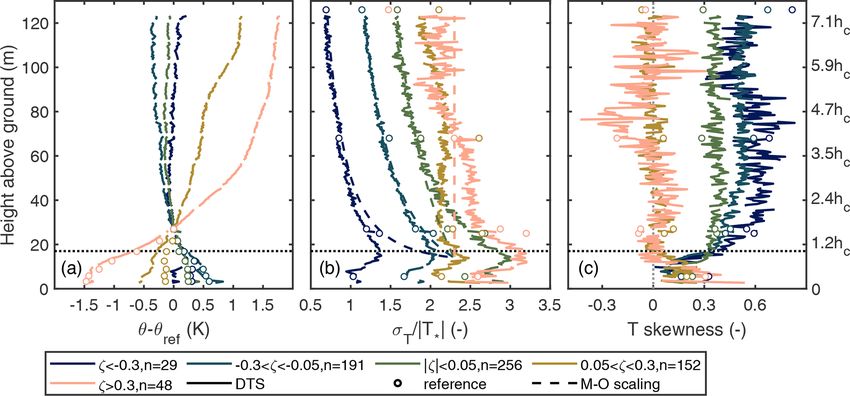
O. Peltola et al.: DTS in forest                                                                                                     2413

where f is frequency and τ is a first-order response time de-           as follows:
scribing the high-frequency response of the system. An es-
                                                                        Ts0 2 = M11 (tl → 0)                                            (9)
timate for the attenuation of the DTS-derived temperature
variance due to imperfect high-frequency response and lower              2 = M11 (0) − M11 (tl → 0).                                 (10)
sampling frequency can be derived by the following:
                                                                        Similarly, the effect of noise on third-order moments can be
       R f2
             TH STT,low df                                              estimated using third-order autocovariance M21 as follows:
        f1
AF =                       ,                                     (6)
                                                                        Ts0 3 = M21 (tl → 0)
             R f3
              f1 STT df
                                                                                                                                      (11)
                                                                         3 = M21 (0) − M21 (tl → 0),                                 (12)
where AF is the attenuation factor, STT is the power spec-
trum measured with the 3D sonic anemometer, STT,low is the              where it was further assumed that the product of Ts0 to any
power spectrum calculated from sonic anemometer data that               power and  to an odd power are zero (Lenschow et al.,
were averaged in the time domain to match the temporal res-             2000). The time series skewness (Sk) was then estimated us-
olution of DTS prior to Fourier transform, and TH was calcu-            ing the second- and third-order moments
                                                                                                        !       calculated with the
lated using a value for τ obtained experimentally with Eq. (5)                                          T 03
(see Sect. 3.2). The integration limits f1 , f2 and f3 are set by       equations above        Sk =    s3/2   . The signal-to-noise ratio
                                                                                                       Ts0 2
the length of the averaging period and the Nyquist frequency
                                                                        was used to estimate the magnitude of noise relative to the
for DTS and 3D sonic anemometer data, respectively. By def-
                                                                        signal as follows:
inition, AF is equal to one for a perfect sensor (τ = 0 s) with
high sampling frequency (i.e. f2 = f3 ), and AF is equal to                       Ts0 2
zero for a fully damped signal (τ → ∞ s).                               SNR =             .                                           (13)
                                                                                  2
Determination of instrument noise
                                                                        3     Results and discussion
Instrument noise can significantly hinder the analysis of
measurements if the signal-to-noise ratio is small. Here,               3.1    DTS instrument noise determination
we utilised the methodology developed by Lenschow et al.
(2000) to extract turbulent statistics from noisy data. The             DTS measurements at high spatial and temporal resolution
method originally developed for lidar data has also been used           contain a significant noise contribution due to the small num-
for EC data (Mauder et al., 2013; Rannik et al., 2016) and              ber of backscattered Raman photons; hence, duplicate or trip-
is part of ICOS EC-data-processing routines (Nemitz et al.,             licate measurements are often conducted. In this study, the
2018). The method has been shown to reliably estimate the               instrument noise was estimated using Lenschow et al. (2000,
influence of noise on second- and third-order statistics in tur-        see Sect. 2.2) for each location along the fibre for each 30 min
bulence measurements in prior studies (e.g. Lenschow et al.,            averaging period. Figure 1 shows the average dependence of
2000; Rannik et al., 2016; Nakai et al., 2020). The fluctuating         the noise standard deviation, σnoise , with length along the fi-
part of the time series T 0 (t) can be thought to consist of sig-       bre, LAF, together with the variability observed in the cali-
nal Ts0 (t) and noise (t) (T 0 = Ts0 + ). All the time series T 0 ,   bration baths. The noise increases exponentially with LAF, as
Ts0 and  have zero means. The second-order autocovariance              expected, since the number of photons available for backscat-
(M11 ) can then be written as follows:                                  tering decreases along the fibre. After taking the mean of
                                                                      the measurements up and down the mast and then averag-
M11 (tl ) = Ts0 +  Ts0 l + l ,                                 (7)    ing over four consecutive points, the average noise decreased
                                                                        from 0.62 to 0.26 K, and was, in practise, independent of the
where overbar denotes time averaging, and subscript l de-               position along the fibre and, thus, height. This decrease is
notes that the time series has been lagged with time lag tl             similar to what would be√expected for fully independent mea-
(Lenschow et al., 2000). Assuming  and Ts0 are uncorrelated            surements (i.e. 0.62 K/ 8 = 0.22 K). This averaging proce-
with each other, it can be found that, in the following:                dure was applied to all further analysis in this study and pro-
                                                                        vided a temperature profile with approximately 0.5 m reso-
M11 (0) = Ts0 2 +  2 ,                                          (8)    lution from 2 up to 120 m above the ground. No temporal
                                                                        averaging was applied in order to preserve the temporal res-
meaning that the time series variance M11 (0) is a sum of sig-          olution of the signal. The noise level after averaging was be-
nal variance Ts0 2 and noise variance  2 . Since noise is as-          low the typical temperature variability measured above the
sumed to be uncorrelated, noise only contributes to the au-             forest canopy during the campaign.
tocovariance at lag zero; hence, the signal variance can be                Based on the fit shown in Fig. 1, the noise at zero LAF
estimated by extrapolating the autocovariance values to zero            was approximately 0.57 K, close to the instrument specifica-
lag, and the noise variance can be estimated from the residual          tions. However, σnoise increased faster as a function of LAF

https://doi.org/10.5194/amt-14-2409-2021                                                      Atmos. Meas. Tech., 14, 2409–2427, 2021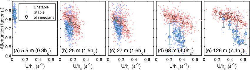
2414                                                                                                      O. Peltola et al.: DTS in forest

Figure 1. Average dependence of noise (1σ ), estimated with               Figure 2. Increase in noise at step losses (i.e. sudden decreases in
Eq. (10), for length along the fibre (LAF) and height above ground        Ps and Pas ) along the cable versus step loss magnitude.
(top x axis). Circles show T variability in the calibration baths
(mean ± SD). Dashed grey line shows the mean T standard devia-
tion measured with 3D sonic anemometer at 27 m height during the          of the obtained values) during the measurement campaign;
measurement campaign. The vertical dotted black lines show the
                                                                          the variability was not fully random as a systematic temporal
limits (bottom and top) of the vertical DTS measurements on the
                                                                −3        component was also evident. Considering Eq. (4), the zero
mast. The black line is a fit (σnoise = 0.57 K + 0.01e8.6×10 LAF ,
                                                                          LAF noise in T is likely related to the variability in laser
R 2 = 0.99) to the noise estimates calculated from the cable going
                                                                          intensity or detector sensitivity. The DTS instrument con-
up (Tup ) and down the mast (Tdown ). The noise level decreased af-
ter averaging the up and down portions of the measurements(Tave ;         tains an internal reference coil of fibre-optic cable used for a
cyan line) and fell below the typical sonic T variability level further   first instrument-based calibration using the variability in the
if four spatially consecutive measurements were averaged.                 Stokes signal (Ps,in ) from this reference coil. We used this as
                                                                          a joint proxy for both the variability in emitted light and de-
                                                                          tector sensitivity, since the signal had not yet experienced any
                                                                          attenuation. The zero LAF noise displayed a linear depen-
than expected, likely due to the experimental setup which                 dence on this proxy (y = (0.10 ± 0.001 K dB−1 )x − (0.44 ±
may have caused mechanical strain on the fibre (cable hold-               0.001) K, R 2 = 0.87, where y equals σnoise at LAF = 0 m,
ers and wind load) and, hence, loss of signal. There were                 and x is the decrease in Ps,in (in decibels) from its maxi-
a few step losses (i.e. sudden decreases in Ps and Pas ; see              mum value). Interestingly, the gradient is similar to that ob-
also Eq. 4) along the cable caused by the support structures,             tained for σnoise increases at step losses (Fig. 2), indicative
and these step losses added to the increases in the noise. The            of a more general dependence between signal intensity and
latter was linearly proportional to the magnitude of the step             σnoise . It is known that laser intensity and detector responsiv-
loss (Fig. 2). In addition to the mechanical stresses on the              ity can be sensitive to changes in temperature; the zero LAF
light-conducting glass core, the increase in noise as a func-             noise showed a non-monotonic dependence on instrument in-
tion of LAF depends on the characteristics of the glass core              ternal temperature (calculated from data originating from the
in the cable and how it is coupled to the outer cable (sheath             internal coil) and displayed additional changes when the in-
and protection). These are specific to the batch of the light-            strument was cooling down or warming up (not shown). The
conducting glass core used during manufacturing of the ca-                dependence was not fully explained by the instrument inter-
ble. Nevertheless, the estimates obtained for instrument noise            nal temperature alone, and further studies are necessary to
along the fibre can be used as a first-order estimate when de-            investigate this more deeply.
signing future DTS measurement campaigns with inevitable
signal artefacts due to the fibre-optic cable.                            3.2   High-frequency response of the DTS system
   The value for σnoise at zero LAF is an intrinsic property of
the measurement device and describes the noise level inde-                The high-frequency response of the DTS system was evalu-
pendently of fibre type or the measurement conditions. The                ated by comparing the power spectra of DTS measurements
variability in the instrument noise at zero LAF was evaluated             against those of the co-located sonic anemometers as a ref-
using a similar fit to that shown in Fig. 1 for each 30 min               erence (Fig. 3). The DTS power spectrum was dominated
measurement period. The obtained zero LAF noise estimates                 by white noise in the high-frequency part of the spectrum,
varied between 0.50 and 0.66 K (fifth and 95th percentiles                whereas the reference followed the canonical inertial sub-

Atmos. Meas. Tech., 14, 2409–2427, 2021                                                     https://doi.org/10.5194/amt-14-2409-2021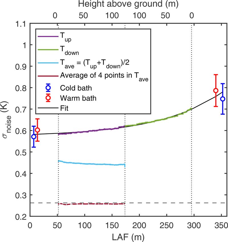
O. Peltola et al.: DTS in forest                                                                                                      2415

                                                                    Table 1. Response times (τ ) describing the high-frequency response
                                                                    of the DTS system derived via comparison with 3D sonic anemome-
                                                                    ters at different heights above ground (see Eq. 5), and attenuation
                                                                    factors (AFs) describing the attenuation of temperature variance due
                                                                    to the high-frequency loss of the signal. A total of 200 estimates for
                                                                    τ were estimated by bootstrap sampling the available data for each
                                                                    height, and the reported values are the medians (interquartile range)
                                                                    of the 200 estimates. AF was estimated for both height-dependent
                                                                    and constant τ for each 30 min time period during the measurement
                                                                    campaign with Eq. (6), and the reported values are the medians (in-
                                                                    terquartile range) of the AF time series.

                                                                      Height           τ                 AF             AF, τ = 2.5 s
                                                                      above           (s)                (–)                 (–)
                                                                      ground
                                                                      (m)
                                                                      5.5       2.9 (2.4...3.5)   0.86 (0.80...0.91)   0.88 (0.83...0.92)
Figure 3. Ensemble-averaged, frequency-weighted and normalised        25        2.3 (2.1...2.4)   0.78 (0.70...0.84)   0.76 (0.69...0.83)
temperature power spectrum estimated from the DTS data and co-        27        3.1 (2.8...3.3)   0.74 (0.67...0.82)   0.76 (0.70...0.83)
located 3D sonic anemometer (reference – REF) at 25 m height          68        2.0 (1.6...2.3)   0.78 (0.66...0.85)   0.78 (0.66...0.85)
above ground (1.5hc , where hc is canopy height). Only periods        126       1.4 (1.0...2.1)   0.85 (0.73...0.90)   0.81 (0.68...0.89)
with high DTS SNR and moderate wind speed (between 1.7 and
3.3 m s−1 ) were selected for the ensemble. The DTS power spec-
trum is shown before and after the noise removal procedure, and
the high-frequency attenuation is demonstrated by multiplying the   conduction within the cable and (3) the spatial and temporal
reference power spectrum with a transfer function (Eq. 5).          sampling resolution of the DTS instrument (Thomas et al.,
                                                                    2012). The latter two can be considered independent of en-
                                                                    vironmental conditions, whereas the first one depends on the
                                                                    depth of the boundary layer surrounding the cable, which is
range slope. Following the commonly applied procedures for          inversely dependent on wind speed. The DTS system high-
EC data processing (e.g. Ibrom et al., 2007), the noise was         frequency response time τ was calculated for different wind
removed from the DTS power spectrum by assuming that it             speed conditions at different heights, and no clear depen-
was not correlated with the signal (see Sect. 2.2) and that         dence on wind speed was found. This indicates that it is likely
the high-frequency response could be estimated from the ra-         that the sampling resolution of the DTS instrument domi-
tio between the noise-removed power spectrum and the 3D             nates the high-frequency response, and hence, τ can be con-
sonic anemometer reference (see Sect. 2.2). Comparing DTS           sidered constant for this particular fibre cable and DTS in-
measurements to sonic anemometers at different heights (Ta-         strument combination.
ble 1) provided slightly different values for the response time        The attenuation of the temperature variance due to the lim-
τ (Eq. 5), likely due to the uncertainty of the noise removal       ited high-frequency response of the DTS system was esti-
procedure. For reference, the values obtained are in the same       mated using the obtained values for τ and Eq. (6). The me-
range as those found for water vapour EC flux measurements          dian values of the calculated AF values for different heights
in high relative humidity conditions (Ibrom et al., 2007;           ranged between 0.74 and 0.86, indicating that the DTS tem-
Mammarella et al., 2009; Runkle et al., 2012) and are sig-          perature variances were typically underestimated by 20 %–
nificantly higher than those for carbon dioxide (Mammarella         30 % (Table 1). The signal attenuation is, in effect, a com-
et al., 2009) or methane (Peltola et al., 2014) EC flux mea-        bination of attenuation (τ ) and turbulent timescales (Horst,
surements. When comparing the DTS power spectra to 3D               1997); hence, AF was not constant while τ was. Turbulent
sonic anemometer power spectra, it is important to recog-           timescales were estimated using roughness sublayer scal-
nise that the instruments were sampling at different rates          ing, i.e. U/hc (Thomas and Foken, 2007a). The turbulent
(DTS with 0.5 Hz and 3D sonic anemometer with 10 Hz), and           timescales are modulated by atmospheric stability; hence,
hence, the power spectra cannot fully be compared across all        AF should also depend on stability. When calculated with
frequencies. The estimated response times and Eq. (5) should        a fixed value for τ for each height, AF showed both an ap-
only be considered as a function for matching DTS and 3D            proximately linear decrease with U/hc and a dependence on
sonic anemometer spectra and not as a transfer function de-         stability (Fig. 4). However, the estimates of AF at differ-
scribing the functioning of the DTS system.                         ent heights did not follow the same linear dependence, with
   Theoretically, the high-frequency response of the DTS            clear differences between the dependence at 68 and 126 m
system depends on (1) heat conduction across the quasi-             (Fig. 4d and e) compared to lower heights, which may indi-
laminar boundary layer surrounding the fibre cable, (2) heat        cate that hc was not the physically meaningful length scale at

https://doi.org/10.5194/amt-14-2409-2021                                               Atmos. Meas. Tech., 14, 2409–2427, 2021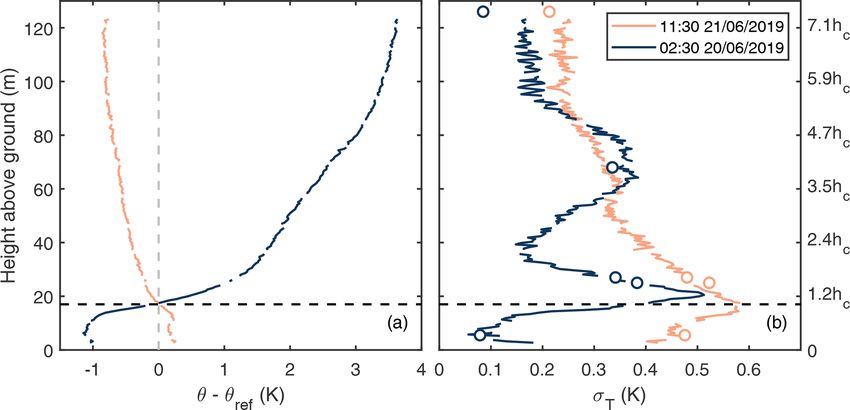
2416                                                                                                    O. Peltola et al.: DTS in forest

Figure 4. Dependence of AF on U/hc at different mast heights. The 30 min values (points), bin medians (filled circles) and the bin in-
terquartile range (error bars) are shown. Data were screened based on flux stationarity (Foken and Wichura, 1996) and values for temperature
variance and w 0 T 0 before plotting (|σT2 | > 0.02 K2 and |w0 T 0 | > 0.015 Km s−1 ).

these heights. The dependence of signal attenuation on tur-             contributing to the vertical turbulent flux. However, within
bulent timescales caused the median AF to increase weakly               the forest canopy, the agreement was worse (Table 2 and
with height above the canopy, indicating smaller signal at-             Fig. 5b). There are at least two reasons for this. (1) There
tenuation well above the canopy (Table 1). However, AF val-             was a 3.5 m horizontal sensor separation between the 3D
ues from different heights were typically within 5 % of each            sonic anemometers and DTS fibre cable, which significantly
other, indicating that the whole profile was attenuated in a            contributed to dampening the high-frequency response of the
similar fashion, and the reported values for AF serve as first-         joint anemometer–DTS flux calculation, especially close to
order estimates for the signal attenuation throughout the pro-          the ground (Horst and Lenschow, 2009). (2) The forest floor
file. Values of AF were higher below the canopy, indicating a           is close, which suppresses the size of eddies dominating heat
reduction in the high-frequency attenuation of the signal; this         transfer, which is also influenced by the canopy elements,
was expected since organised (slow) motions have been pre-              breaking the coherency of large eddies (spectral short cir-
viously found to dominate the scalar variability (and hence             cuit; Finnigan, 2000; Launiainen et al., 2007), and DTS can-
variance) within forests (Thomas and Foken, 2007a, b).                  not capture the small-scale turbulence. This is supported by
                                                                        the finding that the in-canopy temperature variance was cap-
3.3    Second- and third-order statistics                               tured accurately, while the heat flux was not. The temper-
                                                                        ature fluctuations related to the large eddies sweeping into
                                                                        the in-canopy were captured accurately, yet their signal was
Figure 5 and Table 2 show the agreement between tempera-
                                                                        decorrelated with respect to the vertical wind speed (i.e. ver-
ture variances derived from DTS and the co-located 3D sonic
                                                                        tical turbulent flux) by the canopy elements and large hori-
anemometers. Note that statistics derived from 3D sonic
                                                                        zontal sensor separation. This is evident, for instance, in the
anemometers were calculated from sonic temperature and,
                                                                        comparison between, within and above forest canopy power
hence, slightly biased by H2 O fluctuations (see Sect. 2.2).
                                                                        spectra in Launiainen et al. (2007) measured at the same site.
The DTS temperature variance was estimated using Eq. (9),
                                                                        In general, scalars (e.g. temperature) behave very differently
where the noise variance was compensated for prior to the
                                                                        to the vectors within the canopy (Vickers and Thomas, 2014).
comparison. The bulk of the time series variance was re-
                                                                           The third-order statistics, such as temperature skewness,
lated to fluctuations close to the peak of the power spec-
                                                                        were also compared. Again, the effect of noise was removed
tra, and the DTS system was able to resolve the variability
                                                                        following the method by Lenschow et al. (2000), and the
at these frequencies (Fig. 3). Note that the gradient of the
                                                                        temperature skewness values were calculated using Eq. (11).
linear fits between the temperature variance estimates (Ta-
                                                                        Additionally, all data with SNR < 0.5 was discarded for the
ble 2) were close to the values obtained for the attenuation
                                                                        comparison presented in Fig. 5 and Table 2. The reason for
factors describing the high-frequency loss (Sect. 3.2), sug-
                                                                        this additional filtering can be seen in Fig. 6, where the
gesting that the systematic mismatch between DTS and 3D
                                                                        discrepancy between DTS and 3D sonic anemometer tem-
sonic anemometer temperature variances was solely related
                                                                        perature skewness increases rapidly as DTS SNR decreases
to the limited high-frequency response of the DTS system.
                                                                        below 0.5. The dependence of DTS SNR on height meant
   Following Thomas et al. (2012), the kinematic heat fluxes
                                                                        that better estimates of temperature skewness were available
(i.e. w0 T 0 ) were calculated using the vertical wind speed
                                                                        closer to the canopy than at higher elevations above it. Im-
from a 3D sonic anemometer and temperature either from
                                                                        posing a DTS SNR threshold of 0.5 still left 54 % of all DTS
the same 3D sonic anemometer or co-located DTS signal.
                                                                        data measured during the campaign and 63 % of DTS data
Above the canopy, heat fluxes calculated from both sys-
                                                                        measured below 50 m height available for generating third-
tems showed relatively good agreement (Fig. 5e), indicating
                                                                        order statistics. Hence, we conclude that this DTS system
that the DTS system was able to resolve most of the eddies

Atmos. Meas. Tech., 14, 2409–2427, 2021                                                    https://doi.org/10.5194/amt-14-2409-2021
O. Peltola et al.: DTS in forest 2417
Figure 5. Comparison of DTS and 3D sonic anemometer (REF) 30 min values for temperature variance (a, d), w0 T 0 covariance (b, e) and
skewness (c, f) at two different heights on the mast. Upper panels (a–c) show below-canopy heights (0.3hc ) and lower panels (d–f) show
above-canopy heights (1.6hc ). For skewness, only periods with SNR > 0.5 (Eq. 13) were used, otherwise all available data were included.
Coefficients related to the linear fits are given in Table 2. Colour denotes the density of the point cloud. Note that no corrections for sensor
separation effects (Horst and Lenschow, 2009) or signal attenuation (Sect. 3.2) were made prior to comparison.
Table 2. Linear regression statistics between DTS and 3D sonic anemometers at different heights (y = ax + b, where y equals DTS, and
x is a 3D sonic anemometer). The fits between data sets were performed using robust regression in order to minimise the effect of outliers
on the regression coefficients. Standard errors for the coefficients are given in parentheses, and N shows the number of 30 min data points
used in the fit. For skewness, only periods when the signal-to-noise ratio for DTS data was above 0.5 were utilised; for other statistics, all
available data were used. Note that no corrections for sensor separation effects (Horst and Lenschow, 2009) or signal attenuation (Sect. 3.2)
were made prior to comparison.
Height Variance Covariance, w 0 T 0 Skewness
(m) a (–) b (K2 ) N a (–) b (km s−1 ) N a (–) b (–) N
5.5 1.03 (0.003)2418 O. Peltola et al.: DTS in forest
ground level), the measured values for σT /|T∗ | departed from
the M–O predictions. This is typical for the roughness sub-
layer, where the turbulence resembles more mixing layer
than boundary layer turbulence (Raupach et al., 1996; Finni-
gan, 2000; Finnigan et al., 2009), meaning that the turbu-
lent mixing is more efficient than in the surface layer and,
hence, a smaller σT will yield the same turbulent flux. In
other words, the correlation between w and T is higher in
the roughness sublayer than in the surface layer (Patton et al.,
2010), and hence, M–O scaling is no longer valid. These
results suggest that the height of the roughness sublayer at
this site is about 50 m, which corresponds to approximately
3 times the height of the roughness elements (i.e. trees).
This is in line with a previous study at this site (Rannik,
1998) and others, where estimates for the roughness sublayer
height typically range between 2hc and 5hc (3hc being the
most common estimate) (Garratt, 1980; Coppin et al., 1986;
Figure 6. Difference in temperature skewness calculated from 3D Mölder et al., 1999; Poggi et al., 2004; Thomas et al., 2006).
sonic anemometer (REF) and DTS as a function of DTS signal- In near-neutral situations, the scaled temperature variabil-
to-noise ratio (Eq. 13). Individual 30 min values (grey dots), bin ity (σT /|T∗ |) exceeded the predictions made with M–O scal-
medians (circles) and the interquartile range (error bars) are shown.
ing since the heat fluxes (and hence also |T∗ |) decreased with
ζ , yet the temperature variability (σT ) did not decrease at the
same rate. In other words, heat transfer efficiency approached
on the amount of longwave radiative cooling (not shown). zero at the neutral limit (e.g. Rannik, 1998). Under stable
During daytime, DTS showed a weaker decrease in temper- stratification, the scaled temperature variability showed con-
ature with height due to canopy shading; this was particu- sistent z dependence between the displacement height and
larly evident during morning and evening but less so dur- approximately 30 m height, whereas above 30 m it was rel-
ing the middle of the day. The biases in across-canopy tem- atively independent of height, following z-less stratification,
perature differences were 0.07 K (median bias in tempera- and any variability above this height was most likely related
ture difference between 27 and 5.8 m heights) at night and to flow processes other than interaction with the surface.
0.04 K at daytime, indicating that the DTS profile overesti- These observations are in line with previous findings (e.g.
mated the across-canopy temperature gradient at night and Pahlow et al., 2001). Note that, here, |T∗ | was calculated us-
underestimated the gradient during daytime. The unbiased ing measurements at a fixed height (27 m), i.e. local scaling
median temperature gradients during these periods calcu- was not utilised. The profiles shown in Fig. 7b for unstable
lated from the reference measurements, at the heights men- and neutral periods could be expected to show a similar pat-
tioned above, were 0.34 and −0.29 K at night and daytime, tern, even if local scaling were used since turbulent fluxes
respectively. Radiation shields around the cable could have can be conjectured to be constant with height in the bottom
presumably decreased these biases in gradients (Schilperoort part of the ABL. However, for stable situations, the σT /|T∗ |
et al., 2018); however, the usage of screens would have inval- calculated based on local scaling might depart from what is
idated the estimation of turbulent fluctuations from the DTS shown here since |T∗ | varies with z.
data since they disturb the turbulent airflow. Temperature skewness was almost independent of height
As shown above, DTS and 3D sonic temperature mea- (approximately 0.5–0.6) in unstable conditions above 30–
surements showed good agreement in different mixing con- 50 m (2hc –3hc ), which corresponded to the roughness sub-
ditions within the canopy sublayer, slightly above the canopy layer height found above. Skewness increased as the insta-
and well above the forest. As expected, the temperature vari- bility increased. Skewness decreased when moving to the
ance peaked at the canopy top due to (1) strong turbulence canopy sublayer, but stayed positive throughout the profile,
production originating from wind shear and (2) canopy heat indicating non-Gaussian flow. Non-zero skewness is often
source and/or sink related to solar heating (daytime) or ra- connected to an imbalance between the transport of the scalar
diative cooling (nighttime) of the canopy. The scaled tem- in question by ejective and sweeping air motions (Katul
perature variability (σT /|T∗ |, where T∗ was calculated based et al., 2018). Hence, based on these results, the ejections
on Eq. (3) and data from 27 m height) followed Monin– and sweeps were not in balance, and the ejective motions
Obukhov (M–O) similarity scaling in the unstable and near- dominate heat transport in the unstable conditions through-
neutral regime above about 50 m height, indicating that sur- out the air column. Non-zero skewness of scalar time series
face layer scaling was valid between this height and the mast has also been linked to the influence of ABL-scale large ed-
top. As expected, at lower heights (between 50 m height and dies entraining air from the free troposphere and transporting
Atmos. Meas. Tech., 14, 2409–2427, 2021 https://doi.org/10.5194/amt-14-2409-2021O. Peltola et al.: DTS in forest 2419
Figure 7. Profiles of potential temperature gradient (θref = potential temperature at 27 m), normalised temperature variability (σT /|T∗ |) and
temperature skewness derived from DTS (continuous lines) and reference (dots) measurements. The data were binned based on the stability
parameter ζ estimated from EC measurements at 27 m height. For unstable conditions, σT /|T∗ | was also calculated based on Monin–Obukhov
similarity theory (dashed lines) using σT /|T∗ | = 2.3(1 + 9.5|ζ |)−1/3 (Cava et al., 2008). Note that local scaling was not utilised, i.e. |T∗ |
was calculated using measurements at a fixed height (27 m). Only periods with high SNR were used, and n denotes the number of 30 min
periods in each stability bin. The right-hand axis displays height as a fraction of canopy height (hc ), and the canopy height is denoted with a
horizontal dashed line.
it in downdraughts close to the ground (Mahrt, 1991; Cou- By relying on Taylor’s frozen turbulence hypothesis, two-
vreux et al., 2007; van de Boer et al., 2014). In contrast to dimensional spatial details of the large temperature patterns
the profiles in unstable conditions, in stable conditions above can be delineated from the vertical DTS measurements. The
the forest canopy the flow was Gaussian (zero skewness), patterns with low temperatures (related to downward air mo-
whereas skewness was positive below the canopy due to the tions called sweeps) occasionally reached the forest floor but
sweeping motions penetrating through the canopy and bring- did not always penetrate the whole canopy layer (between 10
ing pulses of warm air from aloft into the cold below-canopy and 17 m) since they were likely disrupted by the canopy pas-
air. sage. The patterns with high temperatures, representing up-
ward motions called ejections, typically originated from the
forest floor, traversed the forest canopy and continued mov-
3.5 Examples of organised patterns observed with the ing upwards (compare Fig. 8a and b). Ramp cliff patterns
DTS system across vertical coupling regimes connected to the ejection sweep cycle were evident in the
time series collected just above the canopy (Fig. 8e and f) but
not so clearly at higher levels or below the canopy (Fig. 8c,
The spatially continuous measurements of the DTS system
d and g). These patterns have been previously suggested to
enabled the detection and analysis of spatial temperature pat-
be connected to the wind shear and corresponding inflec-
terns in the flow. During well-developed turbulence, these
tion point instability close to the canopy top (Raupach et al.,
patterns are interlinked with large-scale, organised turbu-
1996; Finnigan, 2000; Cava et al., 2004; Thomas and Foken,
lent air motions (see, e.g., Fig. 3 in Gao et al., 1989). Fig-
2007b; Göckede et al., 2007). For this reason, the signatures
ure 8 shows a measurement example during a daytime un-
of ejections would not be expected to reach very high above
stable regime. Large coherent eddies dominated the flow
the canopy. The mean potential temperature profile (Fig. 9a)
(Fig. 8b), and their signatures on vertical temperature pro-
showed unstable stratification, except below the canopy and
files were captured with the DTS measurements. Positive
in the upper parts of the profile where the stratification was
temperature perturbations were correlated with upward ver-
close to neutral.
tical air motions and negative with downward motions, in-
The patterns observed with the DTS system and the 3D
dicating upward-directed sensible heat flux due to the un-
sonic anemometer at the mast top agreed qualitatively with
stable stratification. The entire 120 m measurement domain
the vertical-pointing wind lidar (Fig. 8), yet quantitative anal-
was coupled due to large coherent eddies effectively mixing
ysis on the agreement was hindered by the fact that the lidar
the air throughout the vertical column. The temporal extent
instrument was located approximately 400 m upwind from
and amplitude of the temperature fluctuations changed with
the measurement mast. While the temporal lag caused by
height, corresponding to changes in the dominant turbulence
this horizontal displacement was taken into account by shift-
timescale and flux magnitude with height.
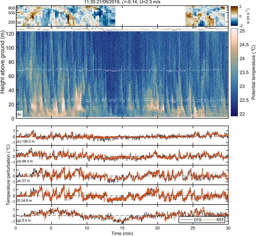
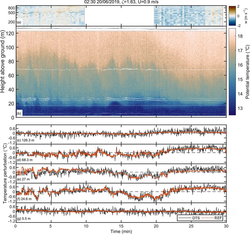
https://doi.org/10.5194/amt-14-2409-2021 Atmos. Meas. Tech., 14, 2409–2427, 20212420 O. Peltola et al.: DTS in forest Figure 8. Example of simultaneous lidar, DTS and 3D sonic anemometer measurements during daytime convective conditions. (a) Lidar vertical wind velocity component (gap is due to non-vertical operation during scanning sequence). (b) Temperature profiles measured with the DTS system (colour) and wind speed fluctuations (arrows) measured with 3D sonic anemometers. For illustration purposes, the wind speed fluctuations were averaged over 10 s, and the vertical wind component was multiplied by 10 prior to plotting. Length of the arrows denote the magnitude of the wind speed fluctuations, and direction is determined by the sign of vertical (w0 ) and horizontal (u0 ) wind speed fluctuations (up – w 0 > 0; down – w0 < 0; left – u0 < 0; right – u0 > 0). (c–g) Temperature perturbations (T − T ) measured with DTS and sonic anemometers at different heights on the mast. Local time (universal coordinated time – UTC+2), the corresponding stability parameter (ζ ) and mean wind speed (U ) measured at 27 m height are given in the figure title. Canopy height was approximately 17 m and is highlighted with a white dotted line in panel (b). For illustration purposes, the data gaps from cable holder locations were filled with linear interpolation prior to plotting. ing the lidar time series in time to maximise the correlation and 10b), resulting from radiative cooling of the forest (net with the mast-top 3D sonic anemometer, the eddies may have radiative loss of 51 W m−2 ) and low mechanical production already been deformed during advection from the lidar mea- of turbulence (i.e. weak wind shear). A total of two strong surement location to the measurement mast, in addition to temperature inversion layers were evident, namely one at the changes in wind direction. Hence, a direct comparison be- canopy top between 12 and 25 m heights and one at 80 m, tween the lidar in its current position and the mast mea- which descended down to 60 m height during the latter part surements is not possible. Nevertheless, these observations of the period (Fig. 11a). Vertical movement of these inversion demonstrate the capabilities of joint measurements with lidar layers resulted in a bimodal vertical profile for σT during this and DTS in capturing a continuous vertical profile of turbu- period (Fig. 9b). These inversion layers decoupled the air col- lence from forest floor up to boundary layer top. umn into the following three layers: below-canopy airspace In contrast to the daytime example, during the nighttime (below 10 m height), canopy layer with organised motions example the air temperature patterns suggested a decoupling (between 10 and 80 m) and a residual layer with slowly vary- caused by the strong thermal stratification of the air (Figs. 9a ing non-turbulent motions (above 80 m). The maximum po- Atmos. Meas. Tech., 14, 2409–2427, 2021 https://doi.org/10.5194/amt-14-2409-2021
O. Peltola et al.: DTS in forest                                                                                                    2421

Figure 9. Mean potential temperature gradient (a) and standard deviation (b) profiles for the two example periods shown in Figs. 8 and 10.
Dots in panel (b) show the σT values estimated with the 3D sonic anemometers at different heights.

Figure 10. Same as Fig. 8 but for a strongly stable situation at night.

https://doi.org/10.5194/amt-14-2409-2021                                                  Atmos. Meas. Tech., 14, 2409–2427, 2021
2422                                                                                                        O. Peltola et al.: DTS in forest

Figure 11. Evolution of potential temperature gradient (dθ/dz) (a) for the nighttime period shown in Fig. 10 and concurrent wind speed time
series from two heights (b). The black dots in panel (a) highlight the location of the maximum gradient at each time step. The gradient was
calculated using spline fit for each time step and estimating the gradient for each height from the first derivative of the fit. White dotted line
shows the canopy height.

tential temperature gradient resided at the canopy height due              temperature observations; for similar observations of wind
to radiative cooling of the canopy (Figs. 9a and 11a). Inverted            vectors, actively heated fibre optics would be needed (Sayde
ramp patterns were observed in the temperature time series at              et al., 2015).
the beginning of the example period (Fig. 10), and a canopy
wave was observed in the middle of the period (Fig. 11a). By
following the evolution of the maximum temperature gradi-                  4    Conclusions and outlook
ent (Fig. 11a), the amplitude of the canopy wave was esti-
mated to be about 8 m. The switch from inverted ramps to                   This study demonstrated the unique observational potential
canopy waves was likely due to a decrease in wind shear and,               of DTS measurements for capturing the salient features of at-
hence, a decrease in turbulence production (Fig. 11b).                     mospheric flow within and above-forest canopies across con-
   These two examples, from contrasting mixing regimes, il-                trasting flow regimes. Despite the fact that these results were
lustrate the unique observational capabilities of the DTS to               obtained with a different DTS machine compared to Thomas
analyse the spatial structure of the organised patterns, which             et al. (2012) and that different cable suspension techniques
can only be guessed at individual heights from classical sonic             were used, these results are in line with their findings on DTS
anemometry (compare, e.g., Fig. 8b and e). In principle, sim-              capturing second-order moments of air temperature variabil-
ilar results could have been obtained with an array of sev-                ity and complement them. In spite of the higher noise floor in
eral in situ instruments (Gao et al., 1989; Lee et al., 1997;              the measurements and the limited high-frequency response
Poulos et al., 2002; Horst et al., 2004; Mahrt and Vickers,                compared to sonic anemometers, we found the DTS tech-
2005; Mahrt et al., 2009; Patton et al., 2010; Bou-Zeid et al.,            nique to accurately capture the second- and third-order mo-
2010; Feigenwinter et al., 2010; Thomas, 2011; Serafimovich                ments, which allows for detection of the spatial structure of
et al., 2011; Mahrt et al., 2014), yet such measurement setups             coherent air motions dominating the temperature variability
do not provide spatially continuous measurements with the                  at the forest–air interface. In accordance with Thomas et al.
same spatial resolution as the DTS system and are labour-                  (2012), the measurements performed best when either large
intensive and require careful cross-instrument calibration.                variability (high heat fluxes) or strong stratification (low mix-
Furthermore, continuous profiles are required for following                ing and clear skies) was present. Cross-canopy temperature
the evolution of, for example, inversion layers (see Fig. 11)              gradients were found to be biased due to radiation-induced
and, hence, not easily detectable with arrays of in situ instru-           errors, especially during morning and evening. These biases
ments. Note, however, that these two examples relied only on               could be reduced with radiation shields around the DTS ca-

Atmos. Meas. Tech., 14, 2409–2427, 2021                                                        https://doi.org/10.5194/amt-14-2409-2021
You can also read