A methodology for attributing the role of climate change in extreme events: a global spectrally nudged storyline
←
→
Page content transcription
If your browser does not render page correctly, please read the page content below
Nat. Hazards Earth Syst. Sci., 21, 171–186, 2021
https://doi.org/10.5194/nhess-21-171-2021
© Author(s) 2021. This work is distributed under
the Creative Commons Attribution 4.0 License.

A methodology for attributing the role of climate change
in extreme events: a global spectrally nudged storyline
Linda van Garderen1 , Frauke Feser1 , and Theodore G. Shepherd2
1 Institute
         for Coastal Research – Analysis and Modelling, Helmholtz-Zentrum Geesthacht,
Max-Planck-Straße 1, 21502 Geesthacht, Germany
2 Department of Meteorology, University of Reading, Reading RG6 6BB, United Kingdom

Correspondence: Linda van Garderen (linda.vangarderen@hzg.de)

Received: 5 June 2020 – Discussion started: 26 June 2020
Revised: 25 September 2020 – Accepted: 26 November 2020 – Published: 18 January 2021

Abstract. Extreme weather events are generally associated           1   Introduction
with unusual dynamical conditions, yet the signal-to-noise
ratio of the dynamical aspects of climate change that are rel-      There is increasing interest in understanding and quantifying
evant to extremes appears to be small, and the nature of the        the impact of climate change on individual extreme weather
change can be highly uncertain. On the other hand, the ther-        and climate events. This is to be distinguished from detect-
modynamic aspects of climate change are already largely             ing the effect of climate change on the statistics of extreme
apparent from observations and are far more certain since           events (IPCC, 2012). In the most commonly used approach,
they are anchored in agreed-upon physical understanding.            changes in the probability distribution of an event class,
The storyline method of extreme-event attribution, which            whose definition is motivated by a historical event, are cal-
has been gaining traction in recent years, quantitatively es-       culated by simulating large ensembles with an atmosphere-
timates the magnitude of thermodynamic aspects of climate           only climate model (Watanabe et al., 2013). The changes are
change, given the dynamical conditions. There are different         computed between the “factual” ensemble, corresponding to
ways of imposing the dynamical conditions. Here we present          observed forcings (e.g. sea-surface temperatures (SSTs) and
and evaluate a method where the dynamical conditions are            greenhouse-gas (GHG) concentrations), and a “counterfac-
enforced through global spectral nudging towards reanalysis         tual” ensemble, corresponding to an imagined world without
data of the large-scale vorticity and divergence in the free at-    climate change. The latter is usually constructed by remov-
mosphere, leaving the lower atmosphere free to respond. We          ing an estimate of the forced changes in SSTs and imposing
simulate the historical extreme weather event twice: first in       pre-industrial GHG concentrations. As discussed by Shep-
the world as we know it, with the events occurring on a back-       herd (2016), this probabilistic approach has two prominent
ground of a changing climate, and second in a “counterfac-          limitations. The first is that every extreme event is unique,
tual” world, where the background is held fixed over the past       but the construction of a general event class blurs the connec-
century. We describe the methodology in detail and present          tion to the actual event and makes it difficult to link the event
results for the European 2003 heatwave and the Russian 2010         attribution to climate impacts. This is important because ex-
heatwave as a proof of concept. These show that the con-            treme impacts are not always associated with extreme me-
ditional attribution can be performed with a high signal-to-        teorology (van der Wiel et al., 2020). The second limitation
noise ratio on daily timescales and at local spatial scales.        is that extreme events are generally associated with extreme
Our methodology is thus potentially highly useful for real-         dynamical conditions, and there is little understanding, let
istic stress testing of resilience strategies for climate impacts   alone agreement, on how those dynamical conditions might
when coupled to an impact model.                                    respond to climate change (Hoskins and Woollings, 2015;
                                                                    Shepherd, 2014). This represents an uncertainty in the prob-
                                                                    abilistic estimates that is difficult to quantify.

Published by Copernicus Publications on behalf of the European Geosciences Union.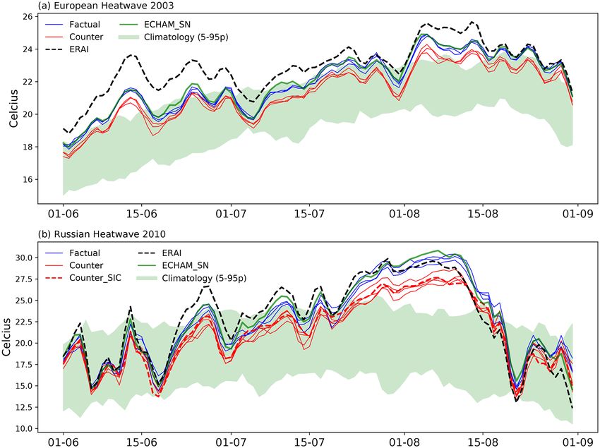
172                   L. van Garderen et al.: A methodology for attributing the role of climate change in extreme events

   On the other hand, thermodynamic aspects of climate             whatsoever, seeks to avoid “Type 1” errors or false alarms
change such as warming and increasing specific humidity            (Lloyd and Oreskes, 2018; Trenberth et al., 2015). A collo-
are robust in sign, anchored in agreed-upon physical un-           quial way of putting this is that rather than asking what ex-
derstanding, and clearly emerging in observations (IPCC,           treme events can tell us about climate change, we ask what
2018). Moreover in many cases the signal-to-noise ratio of         known aspects of climate change can tell us about partic-
the forced dynamical changes appears likely to be small            ular extreme events. Although its results are not expressed
(Deser et al., 2016; Schneider et al., 2012). Thus, although       probabilistically, the storyline approach enables a quantita-
dynamical and thermodynamic processes are interwoven in            tive estimate of climate change with a clear causal interpreta-
the real climate system, it can be useful to regard the uncer-     tion (Pearl and Mackenzie, 2018). Notwithstanding the need
tainties in their forced response to climate change as being       for asking both kinds of questions as they provide different
separable, at least to a first approximation. This has been a      kinds of information (Lloyd and Shepherd, 2020), the story-
growing theme in climate change attribution over the past          line approach is a new development, and there are as yet not
few decades. The distinction between thermodynamic and             so many studies employing this approach.
dynamical changes is not precise, and various ways of im-             In previous applications of the storyline approach, indi-
plementing the separation diagnostically have been used in         vidual extreme weather events have been dynamically con-
different contexts. For extratropical regional climate, it has     strained through boundary conditions applied to a regional
been common to regard the component of change congruent            model (Meredith et al., 2015) or by controlling the ini-
with large-scale internal variability (e.g. as defined by em-      tial conditions in a weather forecast model (Patricola and
pirical orthogonal functions or by self-organizing maps) as        Wehner, 2018). More recently, nudging the free atmosphere
“dynamical” (Deser et al., 2016; Horton et al., 2015) and the      to reanalysis data (leaving the boundary layer free to re-
residual as “thermodynamic”. For tropical climate or for ex-       spond) has been applied in a global medium-resolution at-
tratropical storms, dynamical changes are instead commonly         mospheric model to constrain the dynamical conditions lead-
identified with changes in vertical velocity (Bony et al., 2013;   ing to heatwaves, first to determine the effect of soil mois-
Pfahl et al., 2017). In the absence of evidence to the contrary,   ture changes on selected recent heatwaves (Wehrli et al.,
a reasonable hypothesis is that the forced dynamical changes       2019) and subsequently to determine the effect of past and
are undetectable; this hypothesis is implemented explicitly        projected future warming on the 2018 Northern Hemisphere
in the “pseudo global warming” methodology used for re-            heatwave (Wehrli et al., 2020). The concept of nudging the
gional climate studies (Schär et al., 1996) and in the “dy-        atmospheric circulation in order to impose the dynamical
namical adjustment” methodology used to study observed             conditions has a long history. In particular, spectral nudg-
climate trends (Wallace et al., 2012).                             ing (von Storch et al., 2000; Waldron et al., 1996) allows for
   Trenberth et al. (2015) suggested that the same think-          scale-selective nudging so that only the large spatial scales
ing could be usefully applied to the attribution of individ-       of the model are constrained, while the smaller scales, in-
ual extreme events. Specifically, the extreme dynamical cir-       cluding those relevant to extreme events, are free to be sim-
cumstances leading to the event could be regarded as given,        ulated by the high-resolution model. The climate model can
i.e. arising by chance, and the question posed of how the          thus potentially add value and regional detail to the coarser-
event was modified by the known thermodynamic aspects              resolution forcing dataset. Spectral nudging has been used in
of climate change. This conditional framing of the attribu-        regional climate modelling (Feser and Barcikowska, 2012;
tion question was subsequently dubbed the “storyline” ap-          Scinocca et al., 2015) and in boundary-layer sensitivity stud-
proach (Shepherd, 2016) and has a precedent in the appli-          ies (van Niekerk et al., 2016). Note that in all these modelling
cation of dynamical adjustment to extreme seasonal climate         approaches, the dynamical constraint is imposed “remotely”
anomalies (Cattiaux et al., 2010). As emphasized by Shep-          from the phenomenon of interest (in space, time, and/or spa-
herd (2016) and NAS (2016), there is actually a continuum          tial scale) in contrast to the diagnostic approaches mentioned
between the storyline and probabilistic approaches: story-         earlier and thus preserves the physical interplay between dy-
lines are highly conditioned probabilities, and probabilistic      namics and thermodynamics within the extreme event itself.
approaches generally involve some form of dynamical con-              The purpose of this paper is to provide a methodolog-
ditioning too, through the imposed SST patterns. However,          ical underpinning for the application of large-scale spec-
the extent of conditioning imposed by constraining the at-         tral nudging of divergence and vorticity in a global high-
mospheric state is so severe that in practice the storyline ap-    resolution atmospheric model for the purpose of attributing
proach can be regarded as deterministic, just as weather fore-     the role of thermodynamic aspects of climate change (or
casts, whilst probabilistic in principle, are interpreted deter-   other conditional perturbations) in extreme events of vari-
ministically when the ensemble spread is sufficiently narrow.      ous types and timescales. A key question is to determine
   By focusing on the known effects of climate change, the         what level of refinement of the attribution, in both space and
storyline approach seeks to avoid “Type 2” errors or missed        time, is possible. The outline of the paper is as follows. In
warnings, in contrast to the probabilistic approach, which,        Sect. 2, we elaborate on the technicalities of spectral nudg-
by needing to reject the null hypothesis of no climate change      ing within the ECHAM6 model and its parameter sensitiv-

Nat. Hazards Earth Syst. Sci., 21, 171–186, 2021                                    https://doi.org/10.5194/nhess-21-171-2021
L. van Garderen et al.: A methodology for attributing the role of climate change in extreme events                               173

ities as well as the construction of the counterfactual simu-      only the large-scale fields are nudged. We chose NCEP1 due
lations. In Sect. 3, we exemplify the method by applying it        to its starting date in 1948, which is earlier than any of the
to two well-studied heatwaves: the European 2003 heatwave          other reanalysis data, enabling application of our method
and the Russian 2010 heatwave. As well as identifying some         over a longer period of time. It is conceivable that for certain
important differences between the two events, we examine           kinds of extreme events involving a tight coupling between
the signal-to-noise ratio of our attribution. A concluding dis-    resolved and parameterized processes, ensuring consistency
cussion follows in Sect. 4.                                        between the reanalysis and the model would be beneficial. In
                                                                   a previous application nudging was applied for pressure, tem-
                                                                   perature, vorticity, and divergence (Jeuken et al., 1996) with
2     Method                                                       a constant height profile throughout the entire atmosphere.
                                                                   However, we want to reproduce only the large-scale atmo-
2.1    Spectral nudging
                                                                   spheric circulation and in particular leave the thermodynamic
The spectral-nudging technique is well established within the      fields (temperature and moisture) free to respond; hence we
context of regional climate modelling (Miguez-Macho et al.,        only nudge vorticity and divergence in the free atmosphere.
2004; von Storch et al., 2000, 2018; Waldron et al., 1996).        The aim is to constrain the model as little as possible so that it
In this approach, so-called “nudging terms” are added to           can freely develop small-scale meteorological processes and
the large-scale part of the climate model trajectory, which        extreme events while still achieving an effective control of
draws the model towards reanalysis data. Global spectral           the large-scale weather situation.
nudging (Kim and Hong, 2012; Schubert-Frisius et al., 2017;           The nudging of variable X over time is applied in the spec-
Yoshimura and Kanamitsu, 2008) works in a similar way. It          tral domain as follows (adapted from Jeuken et al., 1996):
constrains large-scale weather patterns of the climate model,      ∂X

                                                                              FX + G (XNCEP − X)     for n ≤ 20, p < 750 hPa
such as high- and low-pressure systems or fronts, to stay             =       FX                     otherwise               ,   (1)
                                                                   ∂t
close to reanalysis data in order to derive a global high-
resolution weather reconstruction. The general idea is that        where X is the variable to be nudged (either vorticity or di-
the realistic large-scale state of the reanalysis data is fol-     vergence), FX is the model tendency for variable X, and
lowed by the global climate model (GCM), while at smaller          XNCEP is the state of that variable in NCEP1. The thresh-
scales the model provides additional detail to improve high-       olds p and n need to be met for nudging to happen, namely
resolution weather patterns. Another merit of the approach is      pressure p must be below 750 hPa, and the spherical har-
the potential to reduce inhomogeneities in the dataset by us-      monic index n must not exceed 20. G is the relaxation coeffi-
ing only a very limited number of variables from the reanal-       cient in units of 10−5 s−1 determining the nudging strength.
ysis data, although this is less of an issue for our application   Nudging is performed at every time step.
because we compare factual and counterfactual simulations             We applied most settings according to Schubert-Frisius
for the same large-scale conditions, so any inhomogeneity in       et al. (2017), including the usage of spectral nudging in
the reanalysis would apply equally to both. For the same rea-      both meridional and zonal directions. We use a plateau
son, our approach can be expected to be robust to any differ-      nudging-strength height profile (see Fig. 1a), which starts at
ences between reanalyses. In order to define a noise level for     750 hPa, then quickly increases up to its maximum nudging
our analysis, we construct small ensembles of three factual        strength, and stays there for higher tropospheric and lower
and three counterfactual simulations. Although such small          and medium stratospheric levels until it again quickly tapers
ensembles are clearly inadequate for quantifying conditional       back to 0 at a height corresponding to 5 hPa. The reason for
probabilities, they have been successfully used in the past        the latter choice is that above 5 hPa there is no NCEP1 re-
(e.g. Shepherd, 2008) to identify robust differences between       analysis data available.
the two ensembles from a deterministic perspective, which is          The strength of nudging is determined by the relaxation
our interest here.                                                 coefficient (G; in 10−5 s−1 ); see Eq. (1). The relaxation co-
                                                                   efficient is often described using the e-folding time (G−1 ;
2.2    ECHAM6 application                                          in 105 s) which represents the simulated time necessary for
                                                                   nudging to dampen out a model-introduced disturbance. For
For this study, we use the high-resolution T255L95 GCM             example, if the e-folding time is 10 h then the nudged model
ECHAM6 (Stevens et al., 2013) with the JSBACH land com-            will dampen out that disturbance (with an assumed amplitude
ponent sub-model (Reick et al., 2013); however the method          of 1) to a value of 1/e and thus greatly reduce it within 10 h.
is applicable to any atmospheric GCM. SSTs and sea ice             A larger relaxation coefficient implies a stronger nudging and
concentrations (SICs) are prescribed from NCEP1 reanalysis         translates into a shorter e-folding time or dampening time
data (Kalnay et al., 1996). ECHAM6 is globally spectrally          (von Storch et al., 2000). We have tested several e-folding
nudged towards the NCEP1 reanalysis data to achieve real-          times to see if the settings could be further relaxed and still
istic weather patterns and extreme events of the past. How-        reproduce the large-scale weather conditions. In Fig. 1b the
ever, any other reanalysis should provide similar results since    impact of the tested e-folding time settings on the temporal

https://doi.org/10.5194/nhess-21-171-2021                                     Nat. Hazards Earth Syst. Sci., 21, 171–186, 2021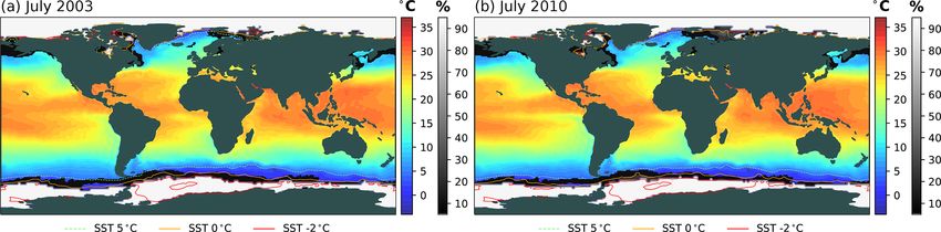
174 L. van Garderen et al.: A methodology for attributing the role of climate change in extreme events
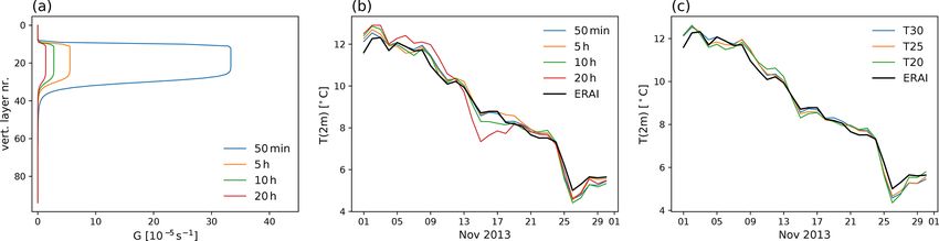
Figure 1. (a) Nudging strength G [10−5 s−1 ] as a function of model level for different choices of minimum e-folding time as indicated.
(b) Daily mean temperatures at 2 m height [◦ C] of ECHAM6 in November 2013 averaged over the European domain (35–60◦ N, 10◦ W–
35◦ E) using the different e-folding times shown in (a) in comparison to ERA-Interim. (c) Daily mean temperatures as in (b) but with a
50 min nudging timescale at different truncations again in comparison to ERA-Interim.
evolution of the 2 m temperature averaged over Europe (35–
60◦ N, 10◦ W–30◦ E) in comparison to ERA-Interim is shown
through November 2013. There is little difference visible be-
tween the 50 min and 5 h e-folding times. The 10 h results
start to show small deviations, whilst the 20 h results deviate
even more noticeably. On the basis of this sensitivity study,
we conclude that the e-folding time can safely be relaxed
from 50 min to 5 h without losing the accuracy of the results.
We similarly aim to limit the range of spatial scales be-
ing nudged as much as possible. In Fig. 1c we show the 2 m
temperature results for the different nudging wavelengths Figure 2. Geopotential height (z500 ) June–July–August (JJA)
in comparison to ERA-Interim. The original T30 settings anomalies [m] for the Northern Hemisphere showing the averaged
used by Schubert-Frisius et al. (2017), which translate to a spectrally nudged dynamic situation over (a) factual members and
minimum wavelength of approximately 1300 km (360◦ /30× (b) counterfactual members of the summer 2010 blocking. Anoma-
lies were calculated relative to the ECHAM_SN 1980–2014 JJA
111 km), show comparable results to the T25 and T20 resolu-
climatology.
tions. The nudging was therefore relaxed to the T20 resolu-
tion, which translates to a minimum wavelength of approx-
imately 2000 km (360◦ /20 × 111 km). This should be suf-
ficient to resolve the large-scale circulation while allowing 2.3 Simulating the counterfactual
smaller-scale processes related to local weather events to de-
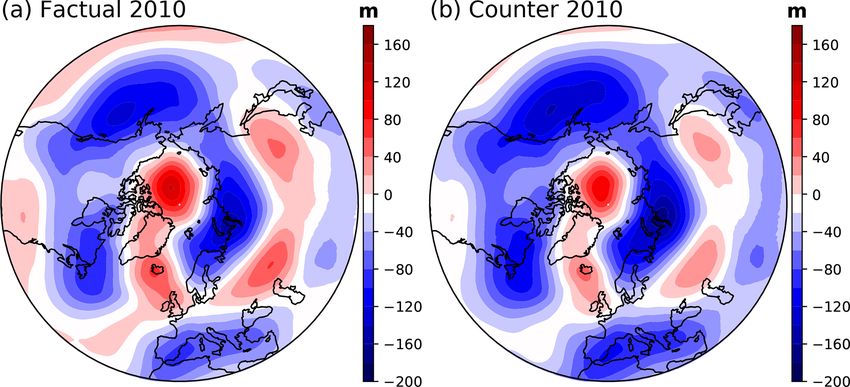
velop freely. In Fig. 2 the geopotential height anomalies for
summer 2010 in the factual and counterfactual simulations In this study, as in probabilistic event attribution, counterfac-
show a strong resemblance. Even though the background tual and factual climate simulations are used to assess the
conditions of the two simulations are different (which is fur- effect of climate change on extreme events. Factual is de-
ther explained in Sect. 2.3), the blocking pattern formed over fined as the world as we know it or a historical simulation.
Russia in 2010 is clearly present in both simulations, demon- Counterfactual is defined as an imagined modern world with-
strating the capability of our nudging method to reproduce out climate change. In our simulations, land use and volcanic
the complex dynamical situation. activity as well as aerosol forcing and sea ice concentration
We used ECHAM_SN throughout this paper to calculate are unchanged between factual and counterfactual. The dif-
climatological data for comparison to our own findings. The ferences between the two worlds are created by altering two
ECHAM_SN dataset is a spectrally nudged global historical important aspects of the simulation: (a) sea-surface temper-
simulation from 1948–2015 (Schubert-Frisius et al., 2017). It ature (SST) and (b) greenhouse gases (GHG). Both worlds
nudged vorticity and divergence towards NCEP1 in a vertical are spectrally nudged in the same way. A potential way to
plateau-shaped profile, equal to the profile we use, at spatial check the results of the counterfactual simulation, especially
scales corresponding to T30 or larger, with an e-folding time for simulations over a longer time span, is to study the con-
of 50 min. sistency between the inferred signals of climate change for
smaller climate forcings (e.g. since mid-century) and the at-
tributed changes in the observational record. Our simulations
are 5 years each and therefore cannot be tested in this way.
Nat. Hazards Earth Syst. Sci., 21, 171–186, 2021 https://doi.org/10.5194/nhess-21-171-2021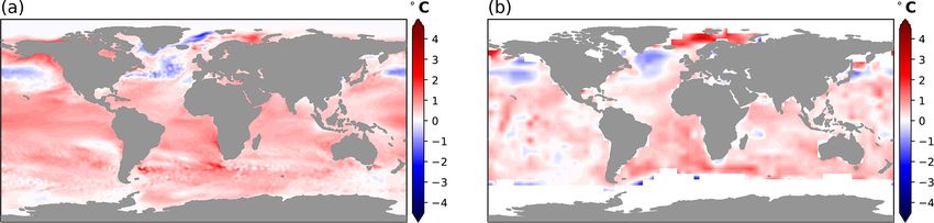
L. van Garderen et al.: A methodology for attributing the role of climate change in extreme events                               175

However for longer simulations such a test would be benefi-         Table 1. Greenhouse-gas concentrations for the ECHAM6 counter-
cial.                                                               factual simulations.
   SST patterns such as the Atlantic Multidecadal Oscilla-
tion or El Niño greatly influence weather extremes. There-                    Greenhouse gas                 Concentration
fore, as with probabilistic event attribution, we impose the                  Carbon dioxide (CO2 )          285 ppmv
same SST variability for both the factual and counterfactual                  Methane (CH4 )                 790 ppbv
simulation, based on the observed SST pattern. (However,                      Nitrous oxide (N2 O)           275 ppbv
this is expected to be less critical in our case since we are                 Chlorofluorocarbons (CFCs)     0
imposing the large-scale atmospheric circulation.) We create
the counterfactual SST conditions by subtracting a climato-
logical warming pattern from the observed pattern, which is
a standard procedure in probabilistic event attribution studies
(Otto, 2017; Vautard et al., 2016; Stott et al., 2016). Although    SIC. This shows that the sea ice edge is well away from the
it is common to consider different climatological warming           European and western Russian domains. Moreover, even un-
patterns as a means of exploring uncertainty, this is not so rel-   der counterfactual conditions the SST remains almost com-
evant in our case since the large-scale circulation is imposed.     pletely physically self-consistent with the SIC according to
The climatological warming pattern is computed using the            the constraints of Hurrell et al. (2008); in particular, there are
ECHAM6 CMIP6 (MPI-ESM1.2-HR) control and historical                 only a very few isolated regions where the SST falls below
simulations at an atmospheric resolution of T127 (Müller et         −2 ◦ C. Nevertheless, we tested the impact of altering SIC
al., 2018). The procedure is shown in Eq. (2):                      in a counterfactual simulation of the Russian heatwave based
                                                                  on the counterfactual SSTs, using the linear relation found by
SSTt,c = SSTNCEP1
               t     −   SST  CMIP6
                              t,h   −  SST   CMIP6
                                             t,pi    ,        (2)   Hurrell et al. (2008). Specifically, SIC was set to 100 % for
                                                                    SSTs below −1.7 ◦ C and to 0 % for SSTs above 3 ◦ C, with
where SSTt,c is the counterfactual SST at time t, SSTNCEP1
                                                      t      is     a linear interpolation in between. The results show no dif-
the NCEP1 SST at time t, SSTCMIP6 t,h   is the CMIP6 historical     ferences compared to the unaltered SIC counterfactual mem-
SST at time t, and SSTCMIP6
                        t,pi   is the CMIP6 pre-industrial SST      bers (see Fig. 5b). However, to apply our method to other
at time t (for the latter, the only relevant time dependence        seasons or regions in close proximity to areas of sea ice loss,
would be seasonal). In our present implementation, which            the counterfactual simulations would benefit from including
targets boreal summer only and concerns only a fairly short         SIC changes in the same way as was done with SST.
time period, the seasonal time dependence is suppressed, and           In the factual simulation the GHGs change according to
the historical CMIP SSTs are taken to be the 2000–2009 av-          observed values (Meinshausen et al., 2011). In the coun-
erage. For a simulation covering a full year the warming            terfactual simulation, GHGs remain at their 1890 values as
pattern should be made seasonal, and for one covering sev-          listed in Table 1. This means that, strictly speaking, our at-
eral decades it would furthermore need to be weighted over          tribution is to the combined effects of anthropogenic climate
time. In Fig. 3 the CMIP6 SST warming pattern shows a               change (including aerosol forcing) recorded in the SSTs as
good resemblance to the observed HadSST3 warming pat-               well as the direct radiative effects of GHG forcing.
tern. The HadSST3 pattern is obtained by subtracting the               The default initial atmospheric state of the ECHAM6
1880–1890 average from the 1980–1990 average SST val-               model is a random state during the simulated mid-1990s.
ues. The general warming and cooling patches in the Pacific         Changing that initial state to a counterfactual initial state re-
Ocean and Atlantic Ocean south of Greenland agree well.             quires a spin-up time to allow the atmosphere and land sur-
Also, the warming north of Scandinavia is clearly visible in        face enough time to reach a new equilibrium state with their
both warming patterns. Despite the observational data-void          new boundary conditions. To accomplish this we run a non-
region east of Greenland and north of Iceland, there is a good      nudged counterfactual spin-up ensemble for 3 model years
resemblance of our modelled warming pattern with observa-           with three members. We chose a 3-year spin-up after con-
tions. Note that pre-industrial SST observations were depen-        firming the soil moisture was adapted to the new counterfac-
dent upon ship records, which in the polar region were very         tual situation (not shown). Each member was initiated at a
few (Rayner et al., 2006), causing this part of the observa-        different starting date (January–March 1995). The results of
tional dataset to be incomplete.                                    these spin-ups are three random atmospheric counterfactual
   For technical reasons, we did not alter the SIC in the           states, which are used as initial conditions for the counter-
counterfactual simulations. Given that the atmospheric cir-         factual experiments. Although in principle both the factual
culation is nudged, changes in SIC are not expected to be           and counterfactual conditions define conditional probabili-
relevant for summertime heatwaves as Arctic amplification           ties, our three-member ensembles are certainly not sufficient
from sea ice loss is a wintertime phenomenon (Screen and            to estimate those probabilities. As noted earlier, our goal here
Simmonds, 2010). In Fig. 4 the counterfactual SSTs for              is simply to determine the robustness of the deterministic dif-
July 2003 and July 2010 are shown together with the factual         ferences between the factual and counterfactual ensembles.

https://doi.org/10.5194/nhess-21-171-2021                                     Nat. Hazards Earth Syst. Sci., 21, 171–186, 2021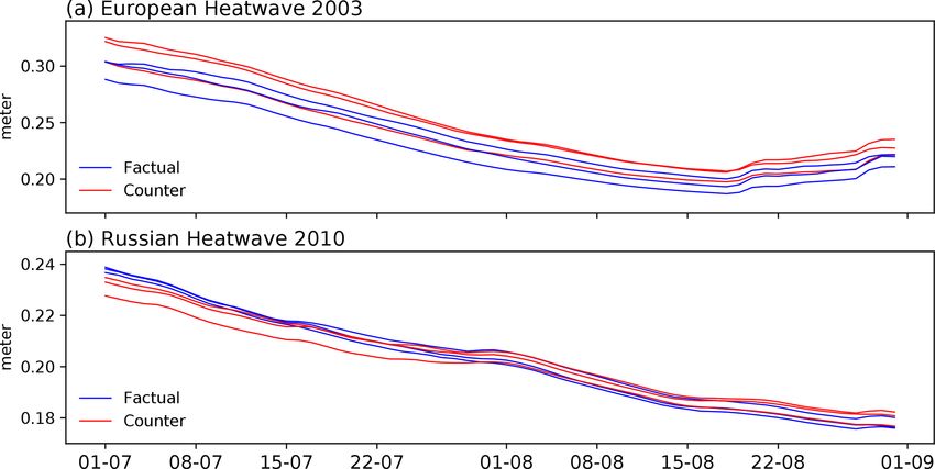
176                    L. van Garderen et al.: A methodology for attributing the role of climate change in extreme events

Figure 3. Sea-surface temperature (SST) warming pattern [◦ C] calculated (a) from ECHAM6 CMIP6 modelled data and (b) from HadSST3
observed data.

Figure 4. Counterfactual SST [◦ C] in shaded colours and factual SIC [%] in greyscale for (a) July 2003 and (b) July 2010. The SST 5 ◦ C
(dashed green), 0 ◦ C (orange), and −2 ◦ C (red) contours are marked for reference.

The ECHAM_SN simulation and the altered SIC simulation                observations we know that the earth has experienced a global
provide out-of-sample tests of robustness for the factual and         warming of approximately 0.7–0.8 ◦ C between preindustrial
counterfactual ensembles, respectively. Figure 5 shows that           times and 2010 (IPCC, 2018). Our modelled global warming,
in both cases, these simulations fall largely within the range        found through the difference between the factual and coun-
of the three-member ensembles.                                        terfactual simulations, thus represents this difference well,
   For the European 2003 heatwave the three counterfac-               albeit with a slight underestimation.
tual members run from 1 March and are initialized with
the spin-up counterfactual atmospheric state members (year
3, March). The three factual members are started 1 month              3     Results
apart from each other (in January–March 2003), and ini-
tialized with the corresponding atmospheric state from the            To illustrate our method, we provide two examples, namely
ECHAM_SN dataset. For the Russian 2010 heatwave the                   the European heatwave of 2003 and the Russian heatwave
three counterfactual members run instead from 1 January be-           of 2010. These events are considered the two strongest Eu-
cause of the known importance of soil preconditioning for             ropean heatwaves on record (Russo et al., 2014, 2015). In
this event (Wehrli et al., 2019). The three factual members           Sect. 3.3 we look deeper into the signal-to-noise ratio of each
again run with 1-month differences in their starting dates,           of the examples and how they compare to each other.
but here from November 2009, December 2009, and Jan-
uary 2010, again initialized with the corresponding state             3.1    European heatwave 2003
from the ECHAM_SN dataset. For analysis regions we se-
lect 35–50◦ N, 10◦ W–25◦ E as the domain for the European             The European summer of 2003 was exceptionally hot and
heatwave 2003 and 50–60◦ N, 35–55◦ E for the Russian heat-            exceptionally dry (Black et al., 2004; Schär et al., 2004;
wave 2010, in line with previous literature (Dole et al., 2011;       Stott et al., 2004). Two heatwaves occurred, a milder one in
García-Herrera et al., 2010; Otto et al., 2012; Rasmijn et al.,       June and an extreme heatwave in August, with peak temper-
2018; Wehrli et al., 2019).                                           atures in France and Switzerland (Black et al., 2004; Schär
   For the summer of 2003, the global temperature difference          et al., 2004; Trigo et al., 2005) but also affecting Portugal,
between factual and counterfactual simulations is 0.64 ◦ C,           northern Italy, western Germany, and the UK (Feudale and
while for the summer of 2010 the difference is 0.66 ◦ C. From         Shukla, 2011a; Muthers et al., 2017). Temperatures exceeded
                                                                      the 1961–1990 average by 2.3–12.5 ◦ C, depending on loca-

Nat. Hazards Earth Syst. Sci., 21, 171–186, 2021                                        https://doi.org/10.5194/nhess-21-171-2021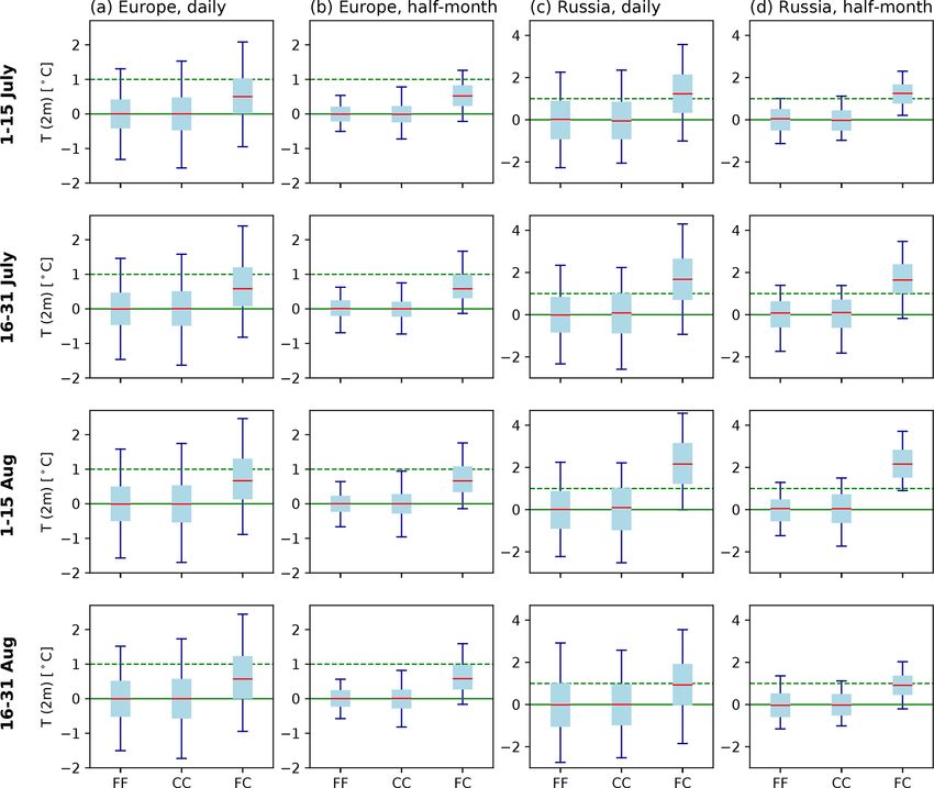
L. van Garderen et al.: A methodology for attributing the role of climate change in extreme events                                 177

Figure 5. Daily mean temperature at 2 m height [◦ C] averaged over (a) Europe (35–50◦ N, 10◦ W–25◦ E) for summer 2003 and over (b) Rus-
sia (50–60◦ N, 35–55◦ E) for summer 2010 for the factual (blue), counterfactual (red), and ECHAM_SN (green) simulations and ERA-
Interim (dashed black) reanalysis data. The climatology (green shaded area) is the 5th–95th ranked percentile range between 1985–2015
calculated with ECHAM_SN (Schubert-Frisius et al., 2017). The dashed red line in (b) shows the simulation with SIC changed in one of the
counterfactual simulations (see text for details).

tion, without much cooling during the night (García-Herrera           out climate change (Hannart et al., 2016; Schär et al., 2004;
et al., 2010; Schär et al., 2004; Stott et al., 2004; Muthers et      Stott et al., 2004). The probabilistic event attribution stud-
al., 2017). The 2003 summer was at that point in time not just        ies show an increased likelihood of the extreme tempera-
the hottest on record (Bastos et al., 2014; Fink et al., 2004), it    tures from increased GHGs (Hannart et al., 2016; Schär et
was the hottest summer in the past 500 years (Luterbacher et          al., 2004; Stott et al., 2004). Other studies focused on the ex-
al., 2004). The consequences were devastating. Estimates ac-          ceptionally high SSTs in the Mediterranean Sea and North
count for 22 000–40 000 heat-related deaths, USD 12–14 bil-           Sea as a cause of reduced baroclinicity, providing an envi-
lion in economic losses, 20 %–30 % decrease in net primary            ronment conducive to blocking (Black et al., 2004; Feudale
productivity (NPP), 5 %–10 % of Alpine glacier loss, and              and Shukla, 2011a, b). By applying the storyline approach,
many more human-health-related issues due to increased sur-           we can consider both causal factors together and shed some
face ozone concentrations (Ciais et al., 2005; Fischer et al.,        additional insight on this event. The dry spring leading up to
2007; García-Herrera et al., 2010).                                   the warm summer conditions was captured by initializing the
   Both the June and August heatwaves were caused by sta-             simulations by 1 March at the latest.
tionary anticyclonic circulations or blocking (Black et al.,             In Fig. 5a, the daily evolution of the domain-averaged
2004). The first block formed in June, then broke and quickly         temperature at 2 m height for June–August for each of
reformed in July, which then caused the second heatwave in            the ensemble members is plotted in comparison to the
August (García-Herrera et al., 2010). However, the extreme            ECHAM_SN 5th–95th-percentile (1985–2005) climatology
temperatures cannot be explained by atmospheric blocking              and ERA-Interim (Dee et al., 2011). The ECHAM_SN
alone. Due to large precipitation deficits in spring that year,       2003 temperature is also plotted for reference and shows a
the heatwaves happened in very dry conditions. The lack of            strong coherence with the factual ensemble, confirming the
clouds and soil moisture caused latent heat transfer to turn          appropriateness of using the ECHAM_SN climatology as a
into sensible heat transfer, which dramatically increased sur-        reference for our factual simulations. The first thing to note
face temperatures (Bastos et al., 2014; Ciais et al., 2005; Fis-      is that the factual and counterfactual ensembles evolve very
cher et al., 2007; Fink et al., 2004; Miralles et al., 2014). It      similarly in time but (except for the third week of June) are
is considered highly unlikely that the 2003 European heat-            well separated, by approximately 0.6 ◦ C, indicating a high
waves would have reached the temperatures they did with-              signal-to-noise ratio at daily resolution for the domain av-

https://doi.org/10.5194/nhess-21-171-2021                                       Nat. Hazards Earth Syst. Sci., 21, 171–186, 2021
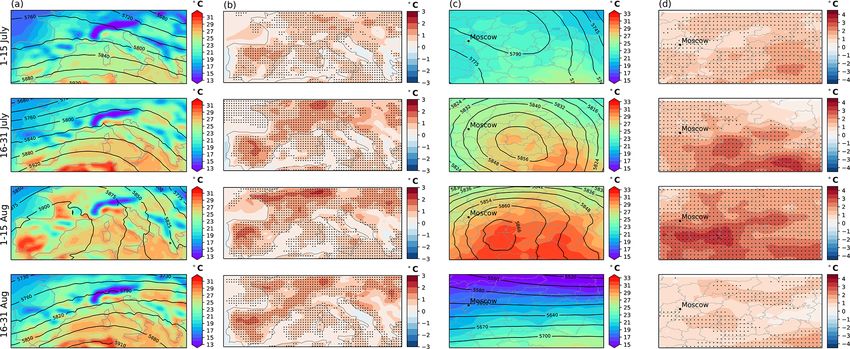
178                     L. van Garderen et al.: A methodology for attributing the role of climate change in extreme events

Figure 6. July and August divided into four half-month periods. Columns (a) and (b) show the European heatwave 2003, while columns (c)
and (d) show the Russian heatwave 2010. In columns (a) and (c), the factual geopotential height at z500 [m] is shown as black contour lines,
while temperatures at 2 m height [◦ C] are shown as shaded fields. In columns (b) and (d), the differences in 2 m temperature [◦ C] between
the factual and counterfactual simulations are shown as shaded fields. Stippling shows where all the factual members are > 0.1 ◦ C above all
the counterfactual members for that grid point. Note that the Russian domain is smaller; therefore the stippling has a different spacing than
in the European domain.

erage. This value of 0.6 ◦ C is in line with the global-mean             and third half-month periods (16–31 July, 1–15 August), the
warming. ERA-Interim and the factual members show a                      temperatures in the factual simulations can locally be up to
strong correlation in time, although the ERA-Interim temper-             2–2.5 ◦ C higher than in the counterfactual simulations, with
atures are higher especially in June and during the heatwave             the differences spread over a large area including Spain, Por-
in the first half of August. The factual temperatures exceed             tugal, France, Germany, Hungary, and Romania. During the
the 95th percentile several times in June–August. In August,             period 1–15 August, which according to Fig. 5a was the
the exceedance lasts for almost 2 weeks, whereas in June it              peak of the heatwave, the hottest area in Europe (Fig. 6a)
does so for approximately 1 week. The counterfactual tem-                is located in south-west France and southern Iberia. However
peratures are not quite so extreme; they exceed the 95th per-            the largest differences between the factual and counterfactual
centile only for a few days at a time in June and August.                simulations (up to 2.5 ◦ C) are found to the north of both of
Nevertheless, it is clear that there would have been a Euro-             these regions, suggesting a shift in the peak temperature. In
pean heatwave in 2003 even without climate change, albeit                the second half of August, there are still some strong temper-
with less extreme temperatures. This analysis thus supports              ature differences visible over most of these regions, although
both of the perspectives on the event discussed earlier whilst           the differences over western France have dampened.
providing a daily resolution of the climate change attribution.             As noted earlier, the dryness of the soil has been identified
   The temperature differences between the factual and coun-             as an important contributing factor to the 2003 heatwave. Our
terfactual ensembles are spatially nonuniform over Europe.               interest here, however, is on whether the soil wetness differed
In Fig. 6a the factual members’ average of the 2 m tempera-              between factual and counterfactual conditions. In Fig. 7a we
ture and of the geopotential height (z500 ) show the meteoro-            see a very similar decline in soil wetness for both the fac-
logical situation averaged over half-month periods following             tual and counterfactual ensemble members from May until
García-Herrera et al. (2010). Figure 6b shows the local dif-             the end of August. The counterfactual simulations start out
ferences in 2 m temperatures between the counterfactual and              with somewhat higher soil wetness than the factual simula-
factual ensemble averages. Stippling is added to each grid               tions, but over the course of the summer the values of both
point where all the three factual members are at least 0.1 ◦ C           sets of simulations move closer towards each other so that
warmer than all the counterfactual members. There is strong              by August the ensembles are close together. Thus it does not
local variance, especially during the heatwave in the first half         appear that climate change had a first-order impact on soil
of August, with differences of up to 2.5 ◦ C. In the first period        wetness in this case.
(1–15 July) the local differences are generally modest, except
in northern Spain, where they reach 1.5–2 ◦ C. In the second

Nat. Hazards Earth Syst. Sci., 21, 171–186, 2021                                           https://doi.org/10.5194/nhess-21-171-2021
L. van Garderen et al.: A methodology for attributing the role of climate change in extreme events                                 179

Figure 7. Average soil wetness in the root zone [m] averaged over Europe in 2003 and Russia in 2010 during July and August of each year.
The factual simulations are shown in blue and the counterfactual simulations in red.

3.2   Russian heatwave 2010                                           atures correlate highly with the counterfactual members,
                                                                      though are somewhat higher at the end of June and begin-
In August 2010 western Russia was hit by an unprecedented             ning of July, and decline much more rapidly following the
heatwave caused by a large quasi-stationary anticyclonic cir-         heatwave halfway through August. Starting after the second
culation, or blocking (Galarneau et al., 2012; Grumm, 2011;           half of July, both the factual and counterfactual temperatures
Matsueda, 2011). It was a heatwave that broke all records             exceed the 95th-percentile climatological temperature, peak
such as temperature anomalies during both day and night,              around 8 August, and return to climatological temperatures
temporal duration, and spatial extent. The effect of soil wet-        around 17 August. This analysis shows that this would have
ness, or rather the lack thereof, on the magnitude of the             been an unprecedented event even without climate change.
temperatures was profound (Lau and Kim, 2012; Rasmijn                 The differences between the factual and counterfactual tem-
et al., 2018; Wehrli et al., 2019; Bastos et al., 2014). The          peratures during the core of the heatwave are noticeably
2010 Russian heatwave is considered the most extreme heat-            higher (about 2 ◦ C) than in the European heatwave 2003, as is
wave in Europe on record (Russo et al., 2015). Approxi-               the spread between the ensemble members. In contrast to the
mately 50 000 lives were lost, 5000 km2 forest burned, 25 %           European case, the anthropogenic warming during the core
of the crop failed and over USD 15 billion worth of economic          of the heatwave is considerably higher than the global-mean
damage was recorded due to this heatwave (Barriopedro et              warming. We attribute both aspects – the greatly enhanced
al., 2011; Lau and Kim, 2012; Otto et al., 2012; Rasmijn et           anthropogenic warming and the larger internal variability –
al., 2018). In some of the attribution studies, the heatwave          to the fact that the Russian domain is much farther inland
was primarily attributed to internal variability as the dynami-       than the European domain, and thus the blocking conditions
cal situation strongly depended on the El Niño–Southern Os-           cut off the influence of the SST forcing and allow a direct
cillation (ENSO) being in a La Niña state (Dole et al., 2011;         radiative effect of GHG increases (Wehrli et al., 2019). Note
Russo et al., 2014; Schneidereit et al., 2012). However, the          that western Russia is known for having large internal vari-
likelihood of the temperatures reaching such extreme values           ability (Dole et al., 2011; Russo et al., 2014; Schneidereit et
has also been assessed as being significantly exacerbated by          al., 2012), which is clearly apparent in our results. It is also
climate change (Otto et al., 2012; Rahmstorf and Coumou,              the case that the Russian domain is smaller than the European
2011). As with the previous example, the storyline approach           domain by a factor of 3.4, which would furthermore tend to
can represent both of these perspectives. Moreover, it over-          increase the variability in the domain-averaged temperature
comes the limitation that the climate models used to perform          shown in Fig. 5.
probabilistic event attribution generally have trouble repro-            The range of temperature differences between factual and
ducing a blocking situation correctly (Trenberth and Fasullo,         counterfactual simulations reach values up to 4 ◦ C locally,
2012; Watanabe et al., 2013).                                         as seen in Fig. 6d. Note that the scale for the Russian heat-
   In Fig. 5b, the daily evolution of the domain-averaged             wave reaches up to 4.5 ◦ C, whereas the scale for the Euro-
temperature at 2 m height for each of the ensemble mem-               pean heatwave reaches only 3 ◦ C. In the first half-month pe-
bers is shown in comparison to ECHAM_SN 2010, the                     riod (1–15 July), when the heatwave had not yet started, the
ECHAM_SN 5th–95th-percentile climatological tempera-                  local temperature differences are between 0.5–2.5 ◦ C, with
tures (1985–2015), and ERA-Interim. ERA-Interim temper-               the maximum differences in the south-east of the domain.

https://doi.org/10.5194/nhess-21-171-2021                                       Nat. Hazards Earth Syst. Sci., 21, 171–186, 2021
180 L. van Garderen et al.: A methodology for attributing the role of climate change in extreme events
Figure 8. Distributions across grid points of differences between ensemble members in temperature at 2 m height [◦ C], separated into the
four half-monthly periods. FF: differences between pairs of factual members; CC: differences between pairs of counterfactual members; FC:
differences between pairs of factual and counterfactual members. The boxes represent the 25th-to-75th-percentile range of the distributions,
the red lines represent the 50th percentiles (the median), and the blue bars indicate the 5th-to-95th-percentile range. The dashed horizontal
line indicates 1 ◦ C for reference. Columns (a) and (b) are for the European 2010 heatwave, and columns (c) and (d) for the Russian 2010
heatwave. Note the different vertical scales for the two events. Columns (a) and (c) show the differences in daily averages, and columns (b)
and (d) show the differences in half-monthly averages.
The temperature differences are largest in the core of the lapping and even cross each other in the beginning of Au-
block region, reaching up to 3.5 ◦ C in the south-east in the gust. These findings are in agreement with those of Hauser
second period (16–31 July) and up to 4 ◦ C in the south, be- et al. (2016), who reproduced the Russian heatwave under
low Moscow, in the third period (1–15 August). The block 1960 conditions and found that the dry conditions occurred
broke in the fourth period (16–31 August) and resulted in a there too, thus concluding they found no direct link between
virtual elimination of the temperature difference. In contrast the drought conditions and climate change. It must be em-
to the European heatwave 2003, here the biggest temperature phasized that this is not to downplay in any way the impact
differences between factual and counterfactual are found in of soil wetness on the event itself, which has been well estab-
the regions with the highest temperatures. lished in the literature. It is only to indicate that the impact
As with the European heatwave 2003, the differences in would have been there even without climate change.
soil wetness do not appear to be of first-order importance
to explain the temperature differences between the factual 3.3 Signal-to-noise analysis
and counterfactual simulations. In Fig. 7b the soil wetness in
the factual simulations is seen to decrease somewhat more The temperature differences found between the factual and
rapidly than in the counterfactual, which could be due to counterfactual simulations are meaningful if they are outside
the higher surface temperature and thus greater evaporation of the internal variability within each ensemble. A different
of soil moisture. However, the soil wetness values are over- way of saying this is that the differences are meaningful if the
two ensembles are distinguishable from each other. To assess
Nat. Hazards Earth Syst. Sci., 21, 171–186, 2021 https://doi.org/10.5194/nhess-21-171-2021L. van Garderen et al.: A methodology for attributing the role of climate change in extreme events 181
this in a statistical manner, temperature differences between approaches to extreme-event attribution, the effect of climate
pairs of factual members (FF), pairs of counterfactual mem- change on the occurrence likelihood of those dynamical con-
bers (CC), and factual–counterfactual pairs (FC) are plotted ditions is not assessed. In that respect, this approach is com-
for each half-month period in Fig. 8. The FF and CC pairs plementary to the more widely used probabilistic event at-
have a median close to 0 and represent the noise level; in tribution. However, since most results of probabilistic event
both cases there are three pairs (F1–F2, F2–F3, F3–F1; C1– attribution appeal in any case to the known thermodynamic
C2, C2–C3, C3–C1). The FC pairs contain the signal; here aspects of climate change, it can be argued that not much
there are nine pairs (F1–C1, F2–C2, F3–C3, F2–C1, F3–C2, is lost in the storyline approach, yet much is gained by the
F1–C3, F3–C1, F1–C2, F2–C3). Each box plot represents the specificity. This is especially the case for extreme events
distribution of 2 m temperature differences across the pairs whose dynamical conditions are not well represented in cli-
and across all grid points. The half-monthly panels represent mate models, e.g. blocking. Spectral nudging enables the re-
distributions of half-month-averaged values, and the daily production of extreme events with their particular dynami-
panels represent distributions of daily values within the half- cal details, allowing the same dynamical events to be repro-
month period. duced in simulations with different boundary conditions and
The daily differences for the European heatwave (Fig. 8a) thereby achieving a high signal-to-noise ratio of the climate
show a median value of about 0.6 ◦ C, irrespective of whether change effect. The combination of both methods – global
the time frame is during the heatwave itself or directly before spectral nudging and the storyline method – thus presents a
or directly after it, consistent with Fig. 5a. Although these are way to quantify, in great detail, the role of known thermody-
not really probability distributions (since they include contri- namic aspects of climate change, together with the specific
butions from different locations within the domain), we can dynamical conditions, in selected extreme events which hap-
use the inter-quartile ranges as measures of signal and noise. pened in the recent past. This can help reconcile the some-
The median difference for FC is above the 75th percentile of times different perspectives on those events that appear in
both CC and FF for daily values, giving confidence that our the literature (some emphasizing climate change, others em-
results are clearly above the noise level. Half-monthly time phasizing internal variability).
averages (Fig. 8b) produce nearly identical median values, We illustrated the method by applying it to two extreme
but we see that the spread is much smaller, as expected. The events that have been the subject of much study: the Euro-
25th percentile of FC now lies above the 75th percentile of pean heatwave of 2003 and the Russian heatwave of 2010.
the CC and FF boxes. By using a small ensemble of both factual and counterfac-
The differences between CF and either FF or CC for the tual simulations, we were able to determine a noise level for
Russian heatwave (Fig. 8c and d) are clearly larger than for our analysis. This revealed that the (conditional) signal of
the European heatwave and in contrast to the European case climate change is determinable at both daily timescales and
vary substantially between the different periods. Consistent local spatial scales. It follows that our methodology could
with Fig. 5b, in the periods outside of the core of the heat- be used to drive climate impact models and thus perform re-
wave (1–15 July, 16–31 August) the median difference be- alistic stress-testing of resilience strategies. With regard to
tween FC is about 1 ◦ C. Inside the core heatwave period the two heatwave examples, our analysis revealed a striking
(16–31 July, 1–15 August), however, the median difference contrast between the two events. In the European heatwave
is more like 2 ◦ C, reaching 2.2 ◦ C for 1–15 August. During of 2003, the effect of climate change was to increase tem-
this latter period the 5th-percentile whisker of half-monthly peratures across Europe by about the global-mean warming
FC differences is above the 75th percentile of FF and CC, level throughout the summer, and the heatwave was simply
which is a very strong signal indeed. When looking at the the dynamical event riding on top of that. In the Russian heat-
results for individual members, the larger internal variabil- wave of 2010, in contrast, the effect of climate change was
ity within the Russian domain (apparent also in Fig. 5b) is much higher than the global warming level and was particu-
clearly visible (not shown), as compared with the European larly enhanced, approximately threefold, during the peak of
case. the heatwave. We interpret this difference as reflecting the
role of direct GHG radiative forcing, which can become ap-
parent when air masses are cut off from marine influence.
4 Discussion and conclusion However, further analysis would be required to confirm this
hypothesis.
We have presented a detailed description and assessment of It is not possible to make a direct comparison between our
a global spectrally nudged storyline methodology to quantify results and probabilistic attribution of these heatwaves be-
the role of known thermodynamic aspects of climate change cause they are answering different questions, and the condi-
in specific extreme weather events. In this methodology, the tionalities are quite different. However, from a methodologi-
particular dynamical conditions leading to the event are taken cal perspective it is useful to contrast the nature of the attri-
as given, i.e. are regarded as random, and the attribution is bution statements that can be made using the different meth-
therefore highly conditional. Thus, as with all such storyline ods. We do this in Table 2 for the case of the Russian 2010
https://doi.org/10.5194/nhess-21-171-2021 Nat. Hazards Earth Syst. Sci., 21, 171–186, 2021182 L. van Garderen et al.: A methodology for attributing the role of climate change in extreme events
Table 2. Example of attribution statements that are possible using the probabilistic and storyline approaches for the case of the 2010 Russian
heatwave.
Probabilistic attribution Averaged over the Russian domain and over the month of July, temperatures in
(based on results from 2010 were 5 ◦ C above the 1960s climatology, of which 4 ◦ C was due to internal
Otto et al., 2012) variability, and 1 ◦ C was due to anthropogenic climate change.
The heatwave represented a 1-in-33-year event, which was 3 times more
likely than it would have been in the 1960s.
Storyline attribution Averaged over the Russian domain, temperatures in 2010 steadily increased from
(based on present results) the 1985–2015 climatology through the month of July until about 10 August, then
rapidly returned to climatology.
The domain-averaged heatwave reached 10 ◦ C above the 1985–2015 climatology
in early August, of which 8 ◦ C was due to internal variability, and 2 ◦ C was due to
anthropogenic climate change.
The anthropogenic component of the warming reached 4 ◦ C in the region to the
south of Moscow during the first half of August, where it exacerbated the already
warm temperatures there.
heatwave. Having said that, there is a continuum between RCM_CMIP6_Historical-HR (last access: 15 January 2021)
storyline and probabilistic approaches (Shepherd, 2016), and (Schupfner, 2021). For analysis we have used the open-access
it is possible to imagine intermediate set-ups which would Python packages.
provide a seamless connection between event attribution and
probabilistic weather prediction (NAS, 2016). These would
need to involve large ensembles (to calculate conditional Author contributions. LvG wrote the article, ran the simulations,
probabilities) and pay more attention to the self-consistency and analysed their results. FF and TGS conceived the study and
contributed to the writing and the interpretation of the results.
of how the counterfactual conditions are imposed. An ex-
ample is the recent use of an operational subseasonal-to-
seasonal prediction system, which involves modifying the at-
Competing interests. The authors declare that they have no conflict
mospheric state and land surface conditions as well as the of interest.
SSTs in generating the counterfactual (Wang et al., 2020).
The nudged global storyline method is an important step
towards a holistic approach within the attribution of individ- Acknowledgements. We would like to thank Sebastian Rast from
ual extreme events, which can quantify the role of both dy- the Max Planck Institute for Meteorology (MPI-M) in Hamburg for
namical variability and known thermodynamic aspects of cli- his technical support in applying spectral nudging in the ECHAM6
mate change and the interplay between them in great spatio- model and Matthias Bittner and Wolfgang Müller from MPI-M
temporal detail. As shown by Wehrli et al. (2020), the method for providing ECHAM6 CMIP6 data. Simulations were carried out
can easily be expanded to a larger number of storylines for on the MISTRAL supercomputer at the German Climate Comput-
both past and future. The method could also be applied to ing Centre (DKRZ), with technical support from Irina Fast. This
other extreme events affected thermodynamically by climate work is a contribution to the “Helmholtz Climate Initiative REK-
change such as tropical cyclones (Feser and Barcikowska, LIM” (Regional Climate Change), a joint research project of the
Helmholtz Association of German Research Centres (HGF), as well
2012). Our future applications are, therefore, intended to
as to the European Research Council advanced grant “Understand-
cover a wide variety of extreme events over the historical ing the atmospheric circulation response to climate change” (grant
record. no. 339390). The authors would like to thank Francis Zwiers and
an anonymous reviewer for their thoughtful and constructive com-
ments which helped improve the manuscript.
Code and data availability. The ECHAM6.1 global atmo-
spheric model is available from the Max Planck Institute for
Meteorology (MPI-M) website: https://code.mpimet.mpg.de/ Financial support. This research has been supported by the Euro-
projects/mpi-esm-users/files (last access: 15 January 2021) pean Research Council (grant no. 339390).
(Giorgetta et al., 2021). The CMIP6 historical simulation data
are archived at the World Data Centre for Climate (WDCC):
https://cera-www.dkrz.de/WDCC/ui/cerasearch/entry?acronym=
Nat. Hazards Earth Syst. Sci., 21, 171–186, 2021 https://doi.org/10.5194/nhess-21-171-2021You can also read