Snow Ensemble Uncertainty Project (SEUP): quantification of snow water equivalent uncertainty across North America via ensemble land surface modeling
←
→
Page content transcription
If your browser does not render page correctly, please read the page content below
The Cryosphere, 15, 771–791, 2021
https://doi.org/10.5194/tc-15-771-2021
© Author(s) 2021. This work is distributed under
the Creative Commons Attribution 4.0 License.

Snow Ensemble Uncertainty Project (SEUP): quantification of
snow water equivalent uncertainty across North America via
ensemble land surface modeling
Rhae Sung Kim1,2 , Sujay Kumar1 , Carrie Vuyovich1 , Paul Houser3 , Jessica Lundquist4 , Lawrence Mudryk5 ,
Michael Durand6 , Ana Barros7 , Edward J. Kim1 , Barton A. Forman8 , Ethan D. Gutmann9 , Melissa L. Wrzesien1,2 ,
Camille Garnaud10 , Melody Sandells11 , Hans-Peter Marshall12 , Nicoleta Cristea4 , Justin M. Pflug4 ,
Jeremy Johnston3 , Yueqian Cao7 , David Mocko1,13 , and Shugong Wang1,13
1 Hydrological Sciences Laboratory, NASA Goddard Space Flight Center, Greenbelt, MD, USA
2 UniversitiesSpace Research Association, Columbia, MD, USA
3 Department of Geography and Geoinformation Sciences, George Mason University, Fairfax, VA, USA
4 Civil and Environmental Engineering, University of Washington, Seattle, WA, USA
5 Climate Research Division, Environment and Climate Change Canada, Toronto, Ontario, Canada
6 School of Earth Sciences and Byrd Polar and Climate Research Center, The Ohio State University, Columbus, OH, USA
7 Department of Civil and Environmental Engineering, University of Illinois at Urbana-Champaign, Champaign, IL, USA
8 Civil and Environmental Engineering, University of Maryland, College Park, MD, USA
9 National Center for Atmospheric Research, Boulder, Colorado, USA
10 Meteorological Research Division, Environment and Climate Change Canada, Dorval, Quebec, Canada
11 Geography and Environmental Sciences, Northumbria University, Newcastle upon Tyne, UK
12 Department of Geosciences, Boise State University, Boise, ID, USA
13 Science Applications International Corporation, Reston, VA, USA

Correspondence: Rhae Sung Kim (rhaesung.kim@nasa.gov)

Received: 26 August 2020 – Discussion started: 15 September 2020
Revised: 15 December 2020 – Accepted: 3 January 2021 – Published: 17 February 2021

Abstract. The Snow Ensemble Uncertainty Project (SEUP)            uncertainty in the SWS estimates due to the large areal extent
is an effort to establish a baseline characterization of snow     over which those estimates are spread. This highlights the
water equivalent (SWE) uncertainty across North Amer-             need for high accuracy in snow estimations across the Tun-
ica with the goal of informing global snow observational          dra. In midlatitude boreal forests, large uncertainties in both
needs. An ensemble-based modeling approach, encompass-            SWE and SWS indicate that vegetation–snow impacts are a
ing a suite of current operational models is used to assess the   critical area where focused improvements to modeled snow
uncertainty in SWE and total snow storage (SWS) estimation        estimation efforts need to be made. Finally, the SEUP results
over North America during the 2009–2017 period. The high-         indicate that SWE uncertainty is driving runoff uncertainty,
est modeled SWE uncertainty is observed in mountainous re-        and measurements may be beneficial in reducing uncertainty
gions, likely due to the relatively deep snow, forcing uncer-     in SWE and runoff, during the melt season at high latitudes
tainties, and variability between the different models in re-     (e.g., Tundra and Taiga regions) and in the western mountain
solving the snow processes over complex terrain. This high-       regions, whereas observations at (or near) peak SWE accu-
lights a need for high-resolution observations in mountains to    mulation are more helpful over the midlatitudes.
capture the high spatial SWE variability. The greatest SWS is
found in Tundra regions where, even though the spatiotempo-
ral variability in modeled SWE is low, there is considerable

Published by Copernicus Publications on behalf of the European Geosciences Union.
772                                                                R. S. Kim et al.: Snow Ensemble Uncertainty Project (SEUP)

1   Introduction                                                      et al., 2008; Guo et al., 2007; Kumar et al., 2017; Mitchell et
                                                                      al., 2004; Mudryk et al., 2015; Murphy et al., 2004; Xia et
Seasonal snow plays an important role in Earth’s climate              al., 2012). An ensemble evaluation can also lead to increased
and ecological systems and influences the number of water             skill by combining a variety of model estimates and allowing
resources available for agriculture, hydropower, and human            the individual model errors to cancel each other out (Xia et
consumption, serving as the primary freshwater supply for             al., 2012). We use the ensemble SWE estimates to assess the
more than a billion people worldwide (Foster et al., 2011).           general spatial and temporal North American SWE charac-
There is a critical need to better understand the role of snow        teristics.
in global climate and land–atmosphere interactions (Brooks               The SEUP ensemble is comprised of 12 ensemble mem-
et al., 2011; Robinson and Kukla, 1985; Stielstra et al., 2015)       bers, created by the combination of four different land sur-
and associated influences on soil moisture, vegetation health,        face models (LSMs) and three different forcing datasets. By
and streamflow (Berghuijs et al., 2014; Ryberg et al., 2016;          using a mix of different LSMs and boundary conditions, the
Stewart et al., 2005). Decreases in total snow water storage          SEUP ensemble captures the uncertainties from both these
can lead to increased droughts (Barnett et al., 2005; Fyfe et         sources. The design of the SEUP ensemble is focused on cur-
al., 2017; Mahanama et al., 2012) and wildfires (Westerling           rent snow capabilities in macroscale modeling, as the land
et al., 2006). In addition, snowmelt is a dominant driver of          models and forcing datasets selected here represent mod-
flooding in many regions of the United States (Berghuijs et           els and datasets currently being employed at key operational
al., 2016).                                                           centers and systems (described in Sect. 2.2). The designed
   Though accurate and timely estimates of snow water                 experiment is conducted at a 5 km spatial resolution for mul-
equivalent (SWE) are required for water and ecosystem                 tiple winter snow seasons (2009–2017). By using a range of
management, obtaining reliable, spatially distributed SWE             forcing products and commonly used operational models, we
has been a challenge, particularly at continental and global          assume that the SEUP ensemble implicitly provides a repre-
scales. At these scales, satellite observations are ideal, but        sentation of both sources of uncertainty. It is likely, however,
global SWE observations remain a major gap in snow re-                that the SEUP ensemble may be deficient in representing the
mote sensing (Dietz et al., 2012; Lettenmaier et al., 2015;           true uncertainty, given the possible errors in boundary condi-
Nolin, 2010), and the US National Research Council com-               tions, model parameters, and model structure. Nevertheless,
mittees of the Decadal Survey (National Academies of Sci-             the SEUP ensemble establishes an important baseline over
ences, Engineering, and Medicine, 2018) identify SWE as               the continental scales to characterize current capabilities and
a missing component of spaceborne water cycle measure-                inform global snow observational requirements. Toward this
ments. This has motivated the advancement of models and               goal, in this article we strive to address several gaps in our
remote sensing techniques to estimate global snow charac-             current understanding of SWE uncertainty with our simu-
teristics (e.g., NASA SnowEx; Durand et al., 2019; Kim et             lation of snow states over the North American continental
al., 2017). Developing the necessary observational methods            domain, including the following questions. (1) Where are
for global coverage while also supporting local snow appli-           the areas of significant uncertainty in SWE? (2) What is the
cations is a significant challenge facing the snow community          seasonality of SWE uncertainty and its spatial distribution?
(Dozier et al., 2016; Lettenmaier et al., 2015). Both mod-            (3) How does uncertainty in SWE vary with key land surface
els and remote sensing techniques are impacted by numer-              characteristics such as vegetation, topography, and snow cli-
ous factors, resulting in significant spatial or temporal errors      mate? (4) How do these regions of high SWE uncertainty
in SWE estimation.                                                    correlate with runoff uncertainties?
   A potential solution to reduce uncertainty associated with            The paper is organized as follows: Sect. 2.1 introduces
any single technique is to combine models and remote sens-            the study area and time period, followed by the descrip-
ing in a data assimilation framework, but this requires an un-        tions of the LSMs and forcing datasets used in this study
derstanding of the underlying uncertainty to be employed.             in Sect. 2.2 and 2.3, respectively. Section 2.4 provides the
In this study, called the Snow Ensemble Uncertainty Project           details about the experimental design, ensemble-based meth-
(SEUP), we apply an ensemble-based land surface model-                ods, and datasets used in the uncertainty evaluation. An eval-
ing approach to establish a baseline characterization of SWE          uation of the SEUP ensemble against a number of reference
and its corresponding uncertainty across North America. The           products is presented in Sect. 3.1. Section 3.2 provides the re-
term “SWE uncertainty” used in this study will refer to the           sults of SWE uncertainty analysis over North America. The
range of SWE estimates across models and is quantified                influence of factors such as topography, snow regime, and
as the ensemble spread. Compared to the use of a single               vegetation type on snow water equivalent/total snow water
model realization, ensemble modeling is generally consid-             storage (SWE/SWS) uncertainty is examined in Sect. 3.3.
ered a better approach to characterize the inherent uncertain-        Section 3.4 discusses how the snow modeling uncertainty
ties in modeling, with the ensemble spread providing a mea-           impacts the uncertainty in the terrestrial water budget com-
sure of the uncertainty in the predictions across models and          ponents. Finally, Sect. 4 provides the major findings and con-
forcing data (Bohn et al., 2010; Dirmeyer et al., 2006; Franz         clusions of this effort.

The Cryosphere, 15, 771–791, 2021                                                          https://doi.org/10.5194/tc-15-771-2021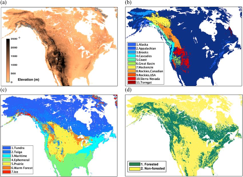
R. S. Kim et al.: Snow Ensemble Uncertainty Project (SEUP)                                                                     773

2     Study area and ensemble configuration                        balance processes. As most land surface models were orig-
                                                                   inally developed to provide the lower boundary conditions
2.1    Study area and time period                                  for global atmospheric models, their applicability is largely
                                                                   assumed to be at coarse spatial scales where the influence
The study area is the North American continental domain            of lateral interactions is negligible. Consequently, similar to
consisting of a 0.05◦ latitude by 0.05◦ longitude equidis-         other model physics components, the snow physics schemes
tant cylindrical grid that extends from 24.875 to 71.875◦ N        in these models are not designed to resolve processes at fine
and 168.625 to 51.875◦ W (Fig. 1a). The glacier regions are        spatial scales (e.g., < 100 m), such as the influence of blow-
excluded from the study domain as the representations of           ing and drifting snow. Further, the complexity of snow meta-
glacier processes are limited in the LSMs used here. These         morphic process representation varies across these models.
glacier exclusions are developed using the Global Land             The snow schemes used in this analysis range from a sim-
Ice Measurement from Space (GLIMS) geospatial glacier              ple single-layer scheme in both Noah2.7.1 and JULES to
database (Raup et al., 2007). The model integrations and           three-layer intermediate complexity schemes in both Noah-
analyses are performed from 2000 to 2017, with the first           MP3.6 and CLSM-F2.5, which greatly influence the snow-
9 years (2000–2009) used as a model spin-up to initialize          pack thermodynamics and the resulting timing and presence
the model’s thermal and hydraulic equilibrium states.              of melt (Dutra et al., 2011). Note that the UKMO currently
                                                                   uses a three-layer scheme in JULES, which was not avail-
2.2    Land surface models (LSMs)                                  able in NASA LIS at the time this study was devised. In or-
                                                                   der to assess current configurations, initial model conditions
The National Aeronautics and Space Administration                  and model parameters used in the operational set-up were not
(NASA) Land Information System (LIS; Kumar et al., 2006;           tuned in this study (Best et al., 2011; Blyth et al., 2006; Clark
Peters-Lidard et al., 2007) is a comprehensive terrestrial         et al., 2011; Ducharne et al., 2000; Ek et al., 2003; Koster et
modeling infrastructure designed to facilitate the efficient       al., 2000; Niu et al., 2011; Yang et al., 2011). The key details
use and assimilation of terrestrial observations. This study       of the model configurations with forcing datasets are sum-
uses a modeling configuration within the NASA LIS that em-         marized in Table S1 in the Supplement.
ploys four different land surface models (LSMs) of varying
complexity at a 5 km spatial resolution over North Amer-           2.3   Forcing datasets
ica: (1) Noah version 2.7.1 (Noah2.7.1; Ek et al., 2003),
(2) Noah-MP version 3.6 (Noah-MP3.6; Niu et al., 2011;             Three different modern forcing datasets are used to drive
Yang et al., 2011), (3) Catchment LSM-Fortuna 2.5 (CLSM-           the models: (1) Modern-Era Retrospective Analysis for Re-
F2.5; Ducharne et al., 2000; Koster et al., 2000), and (4) Joint   search and Applications, version 2 (MERRA2; Gelaro et al.,
UK Land Environment Simulator (JULES, Best et al., 2011;           2017; Molod et al., 2015), (2) Global Data Assimilation Sys-
Blyth et al., 2006; Clark et al., 2011). These models are          tem (GDAS; Derber et al., 1991), and (3) European Centre
selected because all are used operationally at major mod-          for Medium-Range Weather Forecasts (ECMWF; Molteni
eling centers – e.g., Noah2.7.1 is used at the US National         et al., 1996). Original spatial and temporal resolutions for
Centers for Environmental Prediction (NCEP), Noah-MP3.6            these datasets are described in Sect. S2. All models are run
at the National Water Model (NWM), CLSM-F2.5 at the                at 15 min time intervals. To improve the spatial representa-
NASA Global Modeling and Assimilation Office (GMAO),               tiveness of the coarse-resolution meteorological inputs, the
and JULES at the United Kingdom Met Office (UKMO)                  input forcing fields were downscaled to a 5 km grid as fol-
– to provide a baseline of current operational capabilities.       lows. Meteorological inputs of near-surface air temperature,
Note that some of these models do not necessarily represent        relative humidity, surface pressure, and downward longwave
the state-of-the-art approaches for snow modeling, and their       radiation are downscaled by applying a lapse-rate and hyp-
underlying parameterizations may share a similar legacy in         sometric adjustments using the 5 km Shuttle Radar Topogra-
terms of code development. Despite these limitations, how-         phy Mission (SRTM; south of 60◦ N) and the USGS Global
ever, these models and their versions are representative of        30 arcsec elevation (GTOPO30; north of 60◦ N) datasets. The
systems that provide publicly available snow estimates over        lapse-rate correction method follows the approach used in the
continental and global scales. Though the outputs from these       North American Land Data Assimilation System (NLDAS)-
models are used widely for a variety of water resource man-        1 and 2 projects (Cosgrove et al., 2003) where a static en-
agement applications, only a few studies have conducted a          vironmental lapse rate of 6.5 K km−1 is used to apply an el-
careful examination of their differences and limitations, par-     evation adjustment to the coarse meteorological fields. The
ticularly over continental spatial scales.                         downwelling shortwave radiation fields are downscaled us-
   All four LSMs are able to dynamically predict land surface      ing terrain characteristics of slope and aspect as described in
water and energy fluxes in response to surface meteorologi-        Kumar et al. (2013). Over the east- and west-facing slopes,
cal forcing inputs, but they differ in their structural repre-     the slope and aspect-based corrections lead to improvements
sentation of surface and subsurface water, as well as energy       to diurnal processes. Kumar et al. (2013) demonstrated that

https://doi.org/10.5194/tc-15-771-2021                                                      The Cryosphere, 15, 771–791, 2021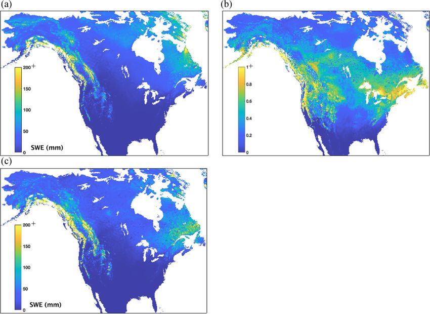
774                                                               R. S. Kim et al.: Snow Ensemble Uncertainty Project (SEUP)

Figure 1. Snow Ensemble Uncertainty Project (SEUP) domain: (a) domain with terrain elevation (gray areas indicate the excluded glacier
regions), (b) individual mountain domains, (c) individual snow class domains, and (d) land cover classification used in this study.

these adjustments are particularly important for improving           rank probability score (CRPS; Matheson and Winkler, 1976),
snow simulations over midlatitude domains in complex to-             which measures the difference between the model and the
pography and concluded that these adjustments should be in-          reference distributions. For computing ER, the ensemble is
cluded in models with resolutions finer than 16 km, but the          first organized in the following order: CLSM-F2.5 (ensem-
adjustments are likely to be small at 5 km resolution. The pre-      ble members 1 to 3), JULES (4 to 6), Noah-MP3.6 (7 to 9),
cipitation fields are downscaled using a variant of the scaling      and Noah2.7.1 (10 to 12), with the order within each LSM
approach of Lenderink et al. (2007) with the high-resolution         being the runs forced with ECMWF, GDAS, and MERRA2
monthly precipitation climatology dataset, WorldClim (Fick           data, respectively. The ensemble SWE at each grid point and
and Hijmans, 2017). The downscaling is performed by fixing           each temporal instance is then sorted and ordered first. The
the ratio of high-resolution precipitation climatology to that       rank of the reference data within this sorted array is then used
of the same climatology at the coarser-scale resolution in or-       as the ER. If the observation is more than 10 % higher than
der to maintain the heterogeneity of the precipitation forcing       the highest ensemble member, then the rank is set to 13. As
fields. The three global datasets are all derived using global       a demonstrative example, if the ensemble SWE values are 1,
atmospheric models that assimilate a large collection of sur-        3, 7, 2, 4, 5, 6, 1, 3, 8, 1, 0 units and the observation has a
face and atmospheric observations and differ primarily in the        value of 5 units, the ER of the observation is set to 9 as the
atmospheric model and assimilation system used.                      sorted array will be 0, 1, 1, 1, 2, 3, 3, 4, 5, 6, 7, 8. Note that
                                                                     the main objective of the ER metric is to examine whether
2.4     Methods                                                      the ensemble encompasses the reference data.
                                                                        CRPS is an often-used performance measure in probabilis-
2.4.1    SEUP ensemble evaluation methods                            tic forecasting, computed using Eq. (1). It provides a mea-
                                                                     sure of the degree of difference between the model distribu-
We use two metrics to evaluate the SEUP ensemble: (1) en-            tion and the observation. CRPS reduces to the mean absolute
semble rank (ER), which ranks the observation relative to            error when used with deterministic (single-member) ensem-
the ensemble providing a measure of how well the ensem-              bles.
ble encompasses a reference observation; and (2) continuous

The Cryosphere, 15, 771–791, 2021                                                          https://doi.org/10.5194/tc-15-771-2021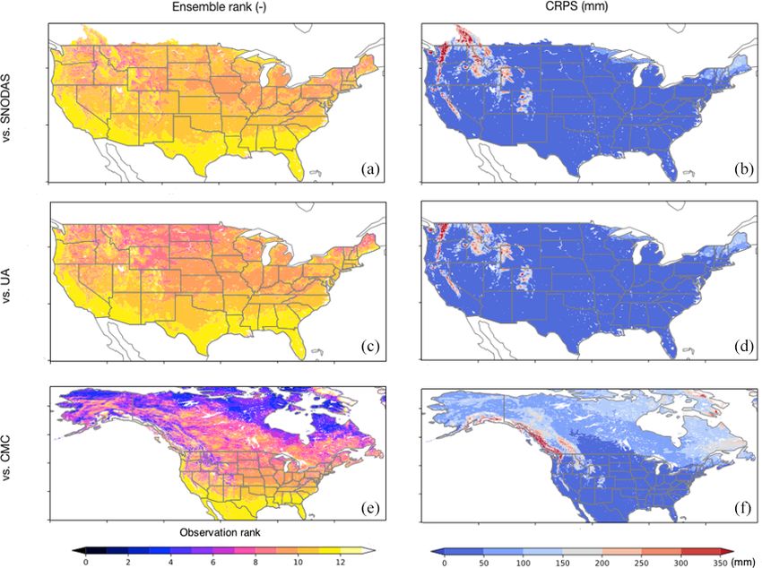
R. S. Kim et al.: Snow Ensemble Uncertainty Project (SEUP)                                                                      775

                                                                   al., 2016; Wrzesien et al., 2017). Despite providing an esti-
                                                                   mate of SWE, in this analysis, we evaluate the CMC modeled
       Z+∞
                                                                   snow depth fields since the CMC only uses snow depth ob-
CRPS =    (Pm − Po )2 dx,                                   (1)    servations in its analysis.
         −∞                                                           A number of ancillary datasets representing topography,
where Pm represents the cumulative distribution function           vegetation type, and snow class are used in stratifying the
(CDF) of the model and Po represents the Heaviside step            spatial dependence of snow uncertainty. First, to treat moun-
function at the observed value. Note that the SEUP ensemble        tainous and non-mountainous regions separately in our study,
size (12) is relatively small, which may affect the resolution     we upscale Wrzesien et al.’s (2018) 1 km binary moun-
of the CDF derived from it. Nevertheless, CRPS provides            tain mask to our 5 km grid (see Fig. 1b). Wrzesien et
an integrated way of capturing the error associated with the       al. (2018) adopted the definition of “mountain” from Kapos
SEUP ensemble when compared to reference measurements,             et al. (2000) based on the elevation, slope, and local relief. In
where a low (good) score indicates a small ensemble spread         their work, the mask was divided into 11 individual moun-
that encompasses the reference observation and a high (bad)        tain domains, which we use here to evaluate SEUP results
score indicates a large spread and/or large difference from        over mountain areas. Table S2 shows the areas of these 11
the observation.                                                   individual mountain ranges.
                                                                      An uncertainty analysis on SWE estimation is performed
2.4.2   Reference and ancillary datasets used in the               across different snow class regions to understand which re-
        uncertainty evaluation                                     gions account for the highest variability. To the best of our
                                                                   knowledge, analyzing uncertainty in SWE estimation across
The reference datasets used for evaluation in SEUP are             different snow classes at continental scales has not been ex-
(1) the daily, gridded snow depth, and SWE analysis from           plored in the literature. In this analysis we use a snow classifi-
the NOAA National Weather Service’s National Operational           cation at a higher (10 km) resolution proposed by Liston and
Hydrologic Remote Sensing Center (NOHRSC) Snow Data                Sturm (A global snow classification dataset for Earth-system
Assimilation System (SNODAS; Barrett, 2003) available at           applications, 2014, unpublished), which analyzes the rela-
30 arcsec spatial resolution; (2) daily gridded estimates of       tionships among textural and stratigraphic characteristics of
snow depth and SWE developed by the University of Ari-             snow layers, climate variables (e.g., air temperature, precipi-
zona (UA; Zeng et al., 2018) available at 4 km spatial resolu-     tation, and wind speed), and vegetation to globally categorize
tion; and (3) the daily, gridded snow depth analysis from the      terrestrial snow into seven classes: Tundra, Taiga, Maritime,
Canadian Meteorological Centre (CMC; Brown and Bras-               Ephemeral, Prairie, Warm forest, and Ice. We downscale this
nett, 2010) available at 25 km spatial resolution. All three       global snow classification dataset to our 5 km model grid
datasets are model-based, but they incorporate in situ mea-        (from the native 10 km spatial resolution). Figure 1c shows
surements from various ground networks. SNODAS analyses            the individual domains of seven snow classes over North
also encompass satellite and airborne measurements, meteo-         America, and Table S3 presents their individual areas.
rological aviation reports, and special aviation reports from         The Moderate Resolution Imaging Spectroradiometer
the World Meteorological Organization (WMO). Though                (MODIS)-derived land cover employing the International
these data are subject to errors, this product provides a con-     Geosphere-Biosphere Programme (IGBP) land cover classi-
sistent, spatially distributed estimate of snowpack conditions     fication method is used to examine the influence of SWE un-
throughout the United States and has been used as a compar-        certainty to vegetation. For simplicity of comparison, we re-
ison dataset in numerous studies (Guan et al., 2013; Meromy        classify the original 17 different land cover classes into two
et al., 2013; Vuyovich et al., 2014). The UA analysis is devel-    classes. These reclassified land cover classes (i.e., forested
oped using an empirical temperature index snow model with          vs. non-forested) are displayed in Fig. 1d, and their areas are
data from networks such as the National Resources Con-             presented in Table S4.
servation Service’s SNOTEL and the National Weather Ser-
vice’s Cooperative Observer Program (COOP). The dataset
was developed to provide a high-resolution, long-term snow         3   Results and discussion
mass product for use in assessing climate change impacts
                                                                   This section presents and discusses results from a range of
(Zeng et al., 2018). SNODAS and UA datasets are available
                                                                   perspectives. Section 3.1 compares the ensemble with the
only over the continental United States, whereas the CMC
                                                                   reference snow datasets. Section 3.2 considers spatial and
data are used for snow evaluation over the entire domain.
                                                                   temporal variation in model uncertainty. Ensemble charac-
While the CMC data have been frequently used for LSM
                                                                   teristics are linked to land surface classification in Sect. 3.3.
evaluation (Forman et al., 2012; Reichle et al., 2017; Takala
                                                                   Finally, the impact of model uncertainty on runoff estimation
et al., 2011), and have been shown to capture interannual
                                                                   is examined in Sect. 3.4.
variability well (Brown et al., 2018), several studies have pro-
vided evidence that the data underestimate SWE (Dawson et

https://doi.org/10.5194/tc-15-771-2021                                                      The Cryosphere, 15, 771–791, 2021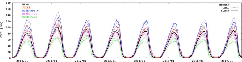
776                                                               R. S. Kim et al.: Snow Ensemble Uncertainty Project (SEUP)

3.1     Evaluation of the SEUP ensemble                              snow time periods in the calculation) for reasons of visual
                                                                     clarity.
To evaluate the snow estimates from the SEUP ensemble,                  The largest spread in ensemble mean SWE is found in re-
three available reference products (described in Sect. 2.4.2)        gions with the deepest snow (see Fig. 3a and c), particularly
are used. Figure 2 shows maps of average ensemble rank               along the northern Pacific coastline. Eastern Canada along
(ER) and average continuous rank probability score (CRPS)            the northern Atlantic coastline and northern Rocky Moun-
(see Sect. 2.4.1) for the SEUP ensemble compared to three            tains also shows a high spread of SWE between ensemble
reference datasets during the time period of 2009 to 2017.           members. These highly complex terrains have relatively high
The examination of ER indicates that in general the SEUP             snowfall precipitation, and the large spread is partially due
ensemble encompasses the three reference measurements. In            to different rain–snow partitioning schemes in each LSM.
the SNODAS comparison, ER values larger than 12 can be               While Noah2.7.1, JULES, and CLSM-F2.5 use a simple tem-
seen in regions with larger snowpacks, such as the Rockies,          perature threshold of 0 ◦ C to distinguish rainfall and snowfall
indicating that over these areas the SEUP ensemble may be            precipitation, Noah-MP3.6 includes a transition temperature
biased low. The ER patterns are similar in both SNODAS and           range described in Jordan (1991) (see Table S1). While our
UA comparisons, though the UA comparison shows more                  lapse-rate correction method is based on approaches used in
spatial variability across different latitudes.                      other products (see Sect. 2.3), the lack of considerations of
   The CRPS comparison provides a measure of the dis-                spatial variability in the snow–rain partition is a limitation,
crepancies between the SEUP ensemble and the reference               particularly over mountainous areas. Similarly, the spatial
datasets. Over most of the domain, including the northeast           distribution of the coefficient of variation shows larger values
and Midwest United States and high plains, the CRPS val-             in areas with the higher ensemble mean SWE and ensemble
ues are low (0–100 mm), where a low (good) score indicates           spread. This indicates that the larger spread is not only due
a small ensemble spread that agrees with SNODAS and UA               to the larger mean SWE in these areas. In addition, Fig. 3b
data. As expected, the largest CRPS values are observed over         also shows significant variability across the middle of North
locations with deep snowpacks, such as the Rocky and Pa-             America, mostly collocated with boreal forest regions con-
cific coastal mountains, where the SEUP ensemble spread is           taining denser vegetation, indicating the handling of vegeta-
greatest. Similar but more muted patterns of disagreement            tion on SWE simulations as another source of dissimilarity
are seen with the CMC data compared to SNODAS and UA                 among the SEUP ensemble members.
over mountainous regions, indicating that the SEUP simula-
tions are more consistent with CMC in those areas. In the            3.2.2   Timing of annual peak SWE
CMC comparison, larger errors are also observed at high lat-
itudes, which are likely caused by a combination of larger           Figure 4 shows spatial maps of the peak SWE (panel a) and
uncertainties in the boundary conditions and model formu-            the highest SWE spread (panel b) along with characteriza-
lations. Relatively good agreement of SEUP with SNODAS               tions of the seasonality of the SWE uncertainty (panels c and
and UA in the ER- and CRPS-based assessments is particu-             d). A measure of the spatial variability on the date of the
larly encouraging, as it provides a measure of confidence that       highest SWE uncertainty is determined by computing the day
the ensemble encompasses reality.                                    of year (DOY) in each water year with the highest ensemble
                                                                     spread and then averaging DOY across the years to identify
                                                                     the times of high and low uncertainty in SWE over North
3.2     SWE uncertainty analysis
                                                                     America. This average DOY of the highest spread is com-
                                                                     pared with the average DOY of the peak SWE to determine
3.2.1    Spatial variability of SWE                                  when the largest variability in the SWE spread occurs within
                                                                     the snow season. The DOY with the greatest SWE spread
An overall assessment of the SWE results is shown in Fig. 3,         ranges from December–April time frame in the lower lati-
which presents the spatial distributions of ensemble mean            tudes to May–June months in the high latitudes (Fig. 4c). In
SWE, the coefficient of variation of ensemble mean SWE,              addition, the seasonality of the greatest SWE uncertainty at
and the range of ensemble mean SWE. Because the seasonal             higher elevations, such as over the Rocky Mountains and the
timing of the greatest SWE and the largest uncertainty in            Pacific coastline, is shifted later in the season as compared to
SWE differ substantially across the North American study             the lower-elevation areas at the same latitude.
domain, we first consider a simple annual mean averaged                 The largest SWE spread is along the northern Pacific
SWE across the entire time period. Seasonal timing of when           coastline and eastern Canada along the northern Atlantic
the greatest uncertainty occurs is deferred to Sect. 3.2.2. For      coastline (Fig. 4a). If the average DOY with the highest SWE
each pixel, the annual ensemble mean SWE is computed by              spread matches that of the peak SWE, it suggests that the
taking an average of 3-hourly SWE from 12 ensemble mem-              largest modeling uncertainty occurs in the peak winter time
bers over the entire study time period. We limit the range of        period. From Fig. 4d, we find that DOYs with the highest
coefficient of variation displayed from 0 to 1 (including no-        SWE spread and peak SWE are very close to each other in the

The Cryosphere, 15, 771–791, 2021                                                         https://doi.org/10.5194/tc-15-771-2021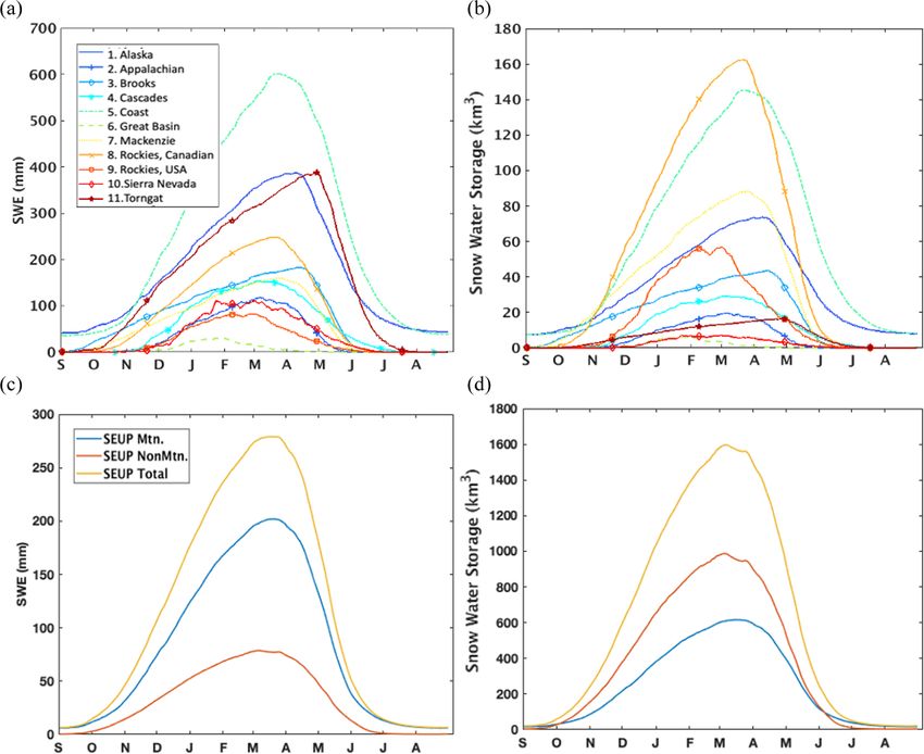
R. S. Kim et al.: Snow Ensemble Uncertainty Project (SEUP)                                                                       777

Figure 2. Maps of average ensemble rank (a, c, e) and average continuous rank probability score (CRPS, mm; b, d, f) from the SEUP
ensemble compared to SNODAS (a, b), UA (c, d), and CMC (e, f). SWE is used for SNODAS and UA comparisons, whereas snow depth
is used for CMC comparison. Ensemble rank represents the rank of the reference data within the SEUP ensemble. Rank 13 represents more
snow than all ensembles, and rank 0 is less snow than all ensembles. CRPS, which is the extension of mean absolute error to ensemble
evaluation, provides a measure of the degree of agreement between the SEUP ensemble and the reference data.

United States over Canada, and the highest SWE spread has            spread in the years of 2010 and 2011 are seen when compar-
a later DOY than that from the peak SWE, indicating that the         ing with other years. At a domain-averaged scale, the largest
largest disagreements in the model estimates are during the          spread in climatological SWE among the ensemble members
melt season. One reason for this could be that the input me-         is seen during the months of February to April and varies by
teorology has larger differences over high latitudes, whereas        as much as ∼ 60 %. In Fig. 5, variability due to model dif-
over the continental United States they are better constrained       ferences (e.g., between solid lines) is generally larger than
due to the greater availability of ground and radar measure-         variability due to forcing data (e.g., between blue lines), con-
ments, resulting in better agreement in the determination of         sistent with Broxton et al. (2016). Figure S1 shows two time
snowmelt regimes.                                                    series of domain-averaged daily mean SWE of the Rocky
                                                                     Mountains and the Cascades in the United States (See Fig. 1b
3.2.3   Interannual variability of SWE                               and Sect. 3.3.1) where the annual snow behavior is known to
                                                                     be well contrasted (Marshall et al., 2019). In the US Rock-
We compare the time series of domain-averaged daily mean             ies, the spread across the ensemble is smaller, and the annual
SWE for each ensemble to examine the temporal variability            maximum SWE is relatively unchanged as compared to those
among the ensemble members (Fig. 5). Interestingly, the in-          of higher elevations in the Cascades.
terannual variability in the peak SWE across the ensemble
is small (see Fig. 5), indicating that the simulated total snow
water storage in North America as a whole did not change
significantly year by year during this time period. Larger

https://doi.org/10.5194/tc-15-771-2021                                                       The Cryosphere, 15, 771–791, 2021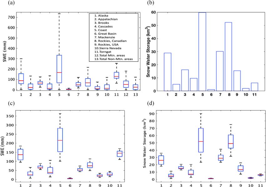
778                                                               R. S. Kim et al.: Snow Ensemble Uncertainty Project (SEUP)

Figure 3. (a) Spatial distributions of ensemble mean SWE, (b) the coefficient of variation of ensemble mean SWE, and (c) the range of
ensemble mean SWE. The ensemble mean SWE is computed by taking an average of 3-hourly SWE from 12 ensembles over the entire study
time period (from 2009 to 2017).

3.2.4   Impact between different LSMs and forcing data               data to be the primary driver of SWE uncertainty in their
        on SWE uncertainty                                           study, with each using a single forcing dataset with added
                                                                     uncertainty and focused on a limited number of relatively
                                                                     small sites mostly in mountainous terrains. Similarly, Yoon
We further examine the influence of models and forcing data          et al. (2019) recently showed that the forcing data drove
on SWE variability by comparing each ensemble grouped by             the uncertainty of model-simulated estimates (i.e., precipita-
LSMs and forcing data. Figure 6 shows the distribution of            tion, evaporation, and runoff) over High Mountain Asia due
domain-averaged, annual mean SWE and indicates that there            to significant differences in the quality of reliable reference
are smaller differences in SWE across the forcing datasets           measurements over the domain. Future efforts should fo-
when driving a common LSM, whereas larger differences                cus on evaluating model parameterizations and snow physics
are seen across the LSMs when driven with a common forc-             schemes such as sublimation, blowing and drifting snow, and
ing data. This finding, from both temporal and spatial analy-        snow–vegetation interactions to identify how representations
ses, indicates that, within our ensemble set, the dominant fac-      of snow physical processes are driving the spread.
tor driving uncertainty in SEUP SWE estimates over North
America is from the LSM. This result is consistent with that         3.2.5   Observational needs
from Mudryk et al. (2015) using an analogous but more lim-
ited ensemble of gridded snow products (cf. Fig. 12 in that          The above results are used to motivate recommendations
paper). Note that both conclusions are based on analysis at          about the spatial and temporal extent to which satellite snow
the continental or hemispheric scale, and there could be dif-        observations may be beneficial. While additional analysis is
ferences at smaller scales and/or in topographically complex         needed to understand and improve the model parameteri-
regions such as mountainous areas. For example, Raleigh              zations that are driving the ensemble spread, remote sens-
et al. (2016) and Günther et al. (2019) showed the forcing           ing observations have the potential to reduce uncertainty

The Cryosphere, 15, 771–791, 2021                                                         https://doi.org/10.5194/tc-15-771-2021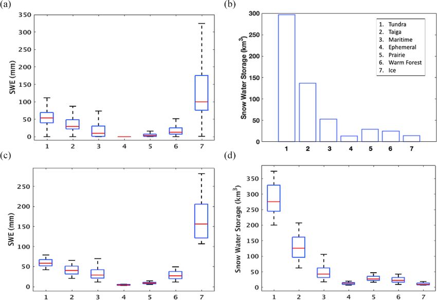
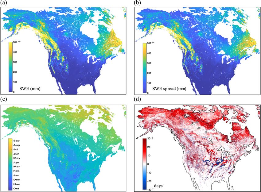
R. S. Kim et al.: Snow Ensemble Uncertainty Project (SEUP)                                                                          779

Figure 4. Spatial distributions of (a) the peak SWE amount, (b) the highest SWE spread amount, (c) the average day of year (DOY) with the
highest ensemble SWE spread, and (d) the difference of average DOY between the highest ensemble SWE spread and the peak SWE (we
are only showing/examining places where the DOY differences exist).

Figure 5. Time series of domain-averaged mean SWE. Different colors and line style were used to represent each ensemble; a bold black
solid line represents the domain-averaged ensemble mean; the units are millimeters.

in global SWE and SWS estimation. For example, from                    snow observations for collecting peak SWE changes with lat-
Sect. 3.2.1 and 3.2.2, the usefulness of observations for re-          itude. Finally, the results from Sect. 3.2.4 suggest that reli-
ducing SWE uncertainty will be higher during the melt sea-             able SWE observations, rather than observations of boundary
son in the high latitudes and western mountainous terrain,             conditions (such as precipitation), may do more to mitigate
whereas having observations in the peak winter is generally            the uncertainties in the current state of snow modeling.
more beneficial in the midlatitudes. Similarly, the timing of

https://doi.org/10.5194/tc-15-771-2021                                                          The Cryosphere, 15, 771–791, 2021
780                                                               R. S. Kim et al.: Snow Ensemble Uncertainty Project (SEUP)

Figure 6. Distribution of North America mean annual average of SWE (i.e., interannual variability), grouped by the LSMs and forcing
datasets (e.g., the box of Noah-MP3.6 represents the distribution of mean SWE, averaged from Noah-MP3.6 runs with all forcing datasets;
the box of MERRA2 represents the distribution of mean SWE, averaged from all LSM runs with MERRA2 forcing data). For the LSM
group, we used eight annual averages of SWE (from 2009 to 2017) for three different forcing datasets (a total of 8 × 3). For the forcing
dataset group, eight annual averages of SWE for four different LSMs (total of 8 × 4) were used. The red line indicates SWE median; top and
bottom of box are the 75th and 25th percentiles, and top and bottom of whiskers represent the maximum and minimum SWE with outliers
(defined as more than 1.5 times the interquartile range, between 25 % and 75 %) omitted.

3.3     Uncertainty analysis for different land                        in the Coast Mountains and the Canadian Rockies, which is
        classifications                                                consistent with the findings of Wrzesien et al. (2018).
                                                                          The variability in the SEUP ensemble spread (i.e., among
In this section, we further explore the uncertainty in North           12 ensemble members) of SWE and SWS across different
American SWE estimates based on different land and snow                mountain ranges is examined in Fig. 7c and d. Similar to
classifications (described in Sect. 2.4.2).                            the spatial variability in SWE (Fig. 7a), the Coast Mountains
                                                                       and Alaska Range have higher uncertainties in SWE among
                                                                       ensemble members, followed by the Cascades, Torngat, and
3.3.1    Uncertainty analysis on different topography
                                                                       the Canadian Rockies. Note that the second highest SWS un-
                                                                       certainty is found in the Canadian Rockies once integrated
We first evaluate the spatial variability of ensemble mean             across the entirety of the mountain range.
SWE within each mountain range. In Fig. 7a, box plots no. 12              To investigate the temporal variability of SWE over dif-
and 13 represent the spatial variability of mean SWE for to-           ferent mountain domains, we compared the mean seasonal
tal mountain areas and non-mountain areas, respectively. To-           cycle of SWE and SWS. Figure 8a and b show the time se-
tal mountain areas are computed by combining the 11 indi-              ries of daily ensemble mean SWE and SWS for each moun-
vidual mountain domains, and all remaining areas are con-              tain range, averaged for a water year. From both comparisons
sidered non-mountain areas. Across the entire continent, the           of SWE and SWS, it can be noted that there is significant
mountain areas show higher spatial variability of SWE and              variability in the timing of peak (and melt) SWE and SWS
higher median SWE than in non-mountain areas (median                   across the mountain ranges. The northern mountain ranges
SWE: 50.17 mm vs. 23.03 mm, ∼ 118 % higher in mountain                 (e.g., Alaska, Brooks, Mackenzie, and Torngat) tend to have
areas). Figure 7a highlights the fact that SWE and its spa-            later dates of peak SWE and SWS, from early April to early
tial variability differ from range to range. For example, most         May, while peak SWE in lower-latitude mountain ranges oc-
coastal mountain ranges (Coast, Alaska, and Torngat) have              curs between February and March. When exploring the time
higher SWE with greater spatial variability than that of con-          series of SWE and SWS for each ensemble, we find that
tinental ranges (Appalachian, Brooks, Great Basin, Macken-             JULES simulates non-seasonal snow in the Alaska Range
zie, and US Rockies), excluding the Canadian Rockies. Com-             and Coast Mountains (even after the glacier exclusions, not
parisons of SWS in each mountain range (Fig. 7b) show that             shown), while other LSMs do not. These different estima-
∼ 50 % of all mountain snow in North America is located

The Cryosphere, 15, 771–791, 2021                                                            https://doi.org/10.5194/tc-15-771-2021
R. S. Kim et al.: Snow Ensemble Uncertainty Project (SEUP) 781
Figure 7. (a) Spatial variability of ensemble mean SWE (in millimeters) within each mountain range. Red line indicates SWE median; top
and bottom of box are the 75th and 25th percentiles, and top and bottom of whiskers represent maximum and minimum SWE with outliers
(defined as more than 1.5 times the interquartile range, between 25 % and 75 %) omitted. (b) Total snow water storage (SWS; in cubic
kilometers) within each mountain range, computed from the average of ensemble mean SWE over the entire time period. The spread of
ensembles for (c) domain- and time-averaged SWE and (d) time-averaged SWS for the different mountain ranges.
tions are likely due to the different snow physics and param- Compared with previous mountain snow studies over
eterizations used in each LSM (see Table S1). The snow sim- North America, the SEUP peak mountain SWS is 1.8 times
ulated in the summer season could explain the higher spread the estimate of 342 km3 from the Canadian Sea Ice and Snow
of SWE seen in the Alaska Range and the Coast Mountains. Evolution Network (CanSISE) data ensemble of Mudryk et
Finally, we use the ensemble mean seasonal cycle of SWE al. (2015) and 0.6 times the estimate of 1006 km3 in Wrze-
and SWS to evaluate differences between mountain areas and sien et al. (2018). For non-mountain areas, the SEUP peak
non-mountain areas of North America. In Fig. 8c and d, we SWS is ∼ 1.5 times the estimate of 678 km3 of the Can-
find that the daily mean SWE is greater in mountain areas SISE data product. The estimated peak SWS over all of North
than in non-mountain areas, while the total daily SWS is America from SEUP is 1604 km3 , which is 47.6 % more than
greater in non-mountain areas than mountain areas. This con- the previous CanSISE estimate (1087 km3 ) and 4.8 % less
trast is due to the significant difference in total area between than the Wrzesien et al. (2018) estimate (1684 km3 ). When
the mountain regions and the non-mountain regions: non- compared with our simulation results, most strikingly, these
mountainous areas cover approximately 5 times more space studies find a lower estimation of SWS even in the non-
than mountainous areas. For total mountain areas, the max- mountain areas, though additional analysis is needed to de-
imum SWE is 202 mm and the maximum SWS is 616 km3 . termine if this is due to resolution differences or some other
Alternatively, total non-mountain areas have 79 mm of max- influence. The CanSISE SWE estimate is produced using
imum SWE and 988 km3 of maximum SWS; i.e., mountain a somewhat similar ensemble mean approach of SEUP, by
areas have deeper snow, whereas more snow is stored in non- combining observations and model estimates at 1◦ spatial
mountainous areas. resolution. Therefore, the lower estimate of SWS in the Can-
SISE data product might be explained by their coarser spa-
https://doi.org/10.5194/tc-15-771-2021 The Cryosphere, 15, 771–791, 2021782 R. S. Kim et al.: Snow Ensemble Uncertainty Project (SEUP) Figure 8. (a) Climatological SWE (in millimeters) within each mountain range, computed from domain ensemble mean SWE over a water year. (b) Total snow water storage (SWS; in cubic kilometers) climatology within each mountain range, computed from domain ensemble mean SWS over a water year. The mean seasonal cycle of domain-averaged SWE (c) and SWS (d) for mountain areas, non-mountain areas, and North America. tial resolution compared to the simulation resolution of this estimated due to the coarse modeling resolution, especially study (i.e., at 5 km). Studies such as Broxton et al. (2016) in mountain areas. Since Wrzesien et al. (2018) used Can- have highlighted the systematic underestimation of SWE SISE for non-mountain SWS estimates, it is possible that from global reanalyses and continental-scale LDASs as a their partitioning of mountain versus non-mountain snow is key issue. Previous studies also highlighted the limitations overestimated. In addition, while SEUP employs ensemble of coarse-resolution models, particularly in capturing snow model simulations over an 8-year time period, Wrzesien et accumulation in mountain areas, and suggested using a reso- al. (2018) simulated the mountain snowpack using a single lution of < 10 km (Ikeda et al., 2010; Kapnick and Delworth, regional climate model (i.e., the Weather Research and Fore- 2013; Pavelsky et al., 2011; Wrzesien et al., 2017). casting Model, WRF version 3.6, Skamarock et al., 2008; Despite similar identical total North American SWS esti- coupled to the Noah-MP3.6, Niu et al., 2011) forced by ERA- mation between SEUP and Wrzesien et al. (2018), there are Interim for a “representative year” (i.e., different single year significant differences in the partitioning between mountain for each mountain range). This proposed “representative cli- and non-mountain SWS. SEUP estimates that 60 % of all matology” was used at spatial resolutions of 27 and 9 km continental snow is located in non-mountains, while Wrze- for the outer and inner domains, respectively. One possi- sien et al. (2018) gave an estimation of 60 % of all continen- ble reason for their higher SWS estimates in mountain areas tal snow in mountains. The CanSISE results suggested that (∼ 63 % greater than SEUP) is that their representative year ∼ 75 % of all continental snow is located in non-mountains, had more snow compared with our average climatology ap- though as noted above, CanSISE estimates may be under- proach over the entire study period, which included low snow The Cryosphere, 15, 771–791, 2021 https://doi.org/10.5194/tc-15-771-2021
R. S. Kim et al.: Snow Ensemble Uncertainty Project (SEUP)                                                                      783

(drought) years. Another reason why Wrzesien et al. (2018)          different snow classes. Both our spatial variability analysis
had more snow in the mountain is because they used a high-          and uncertainty analysis among ensemble members of SWE
resolution (9 km) atmospheric model. The coarser-resolution         and SWS estimates provide new insights on the relative im-
atmospheric models generally do not simulate enough snow-           portance of different snow classes; the Tundra region has the
fall in the mountains due to their inability to resolve the com-    greatest total SWS and large ensemble spread in those esti-
plexity of the topography (Lundquist et al., 2019). The use of      mates between models; Taiga and Maritime regions also have
a different glacier mask is another possible explanation for        a significant fraction of the total North American SWS and
this discrepancy. Note that any change in total water storage       show high variability in SWE estimates likely due to LSM
from GRACE data is not solely due to snow accumulation or           handling of vegetation impacts, such as canopy interception
melt. We also compare the variability of SWS among differ-          and sublimation. The SEUP results indicate that SWE es-
ent LSM simulations (not shown) and find that the highest           timates in the Tundra region are more consistent between
mountain SWS (812 km3 ) was estimated from Noah-MP3.6               ensemble members, likely because the vegetation is sparse
simulations while Wrzesien et al. (2018) showed the SWS es-         there; however, given the large areal extent, accurate SWE
timate of 1006 km3 from their simulation of WRF 3.6 using           estimates are especially critical in estimating total SWS in
Noah-MP. Note that the Noah-MP3.6 is the most recent and            the Tundra region. Further, we note that the Tundra region
advanced model among SEUP LSMs and has been shown                   is subject to snow erosion and sublimation losses, two pro-
to perform better in previous studies (e.g., Wrzesien et al.,       cesses that the LSMs used in this study do not explicitly sim-
2015).                                                              ulate. These results point to the need for high accuracy in
   Overall, the analysis of SWE uncertainty over different          shallow snow observations that cover large regions, such as
topographical regimes confirms that mountain ranges have            Tundra or Prairie, while high spatial resolution in these areas
greater SWE variability among ensemble members than non-            may be less important; the high resolution of SWE observa-
mountain regions, likely due to the methods used by the mod-        tion is more suitable for vegetated areas such as Taiga and
els to resolve the complex and spatially variable processes         Maritime.
over such terrain and the ability of forcing data to capture
orographic effects. These limitations should be addressed           3.3.3   Influence of vegetation on SWE uncertainty
through further evaluation of the differences and capabilities
of LSMs to simulate mountain snow and may also benefit              An assessment of snow estimation uncertainty as a function
from observational data at a high spatio-temporal resolution        of vegetation is presented in this section. Here we focus pri-
over such areas. Further, as noted above, there are still signif-   marily on the differences in snow simulations over forested
icant disagreements in the current understanding of the basic       and non-forested areas, since forest snow processes are a
partition of SWE and SWS between mountainous and non-               model feature that is handled differently between models
mountainous regions, caused by a variety of factors which           (Rutter et al., 2009). The forest category includes the ever-
are not easy to resolve.                                            green forest, deciduous forest, and mixed forest land cover
                                                                    classes, whereas the non-forest category captures the rest of
3.3.2   Uncertainty analysis stratified by snow classes             the land cover categories of Fig. 1d. The spatial variations
                                                                    in ensemble mean SWE as well as the ensemble mean SWS
The distribution of ensemble mean SWE and SWS (Fig. 9a              for forested and non-forested areas are shown in Fig. 10a and
and b) was computed over the entire time period using the           b, respectively. Figure 10a indicates that the non-forested re-
snow class definitions that are shown in Fig. 1. Across the         gions have larger spatial variability than the forested areas.
entire continent, the Ice region shows the highest estimate of      The larger spatial variability in SWE over the non-forested
SWE with the highest spatial variability, followed by Tundra,       regions is likely explained by the differences in the areal cov-
Taiga, Maritime, Warm Forest, Prairie, and Ephemeral re-            erage of forests and non-forests (Fig. 1d). The bar plot in
gions. Higher latitudes tend to have higher estimates of SWE        Fig. 10b shows that 66 % of snow in North America is lo-
and greater spatial variability. Non-seasonal snow was esti-        cated in the non-forested regions.
mated in the Ice region, even though glaciers were excluded,           Figure 10c and d show the uncertainty in SWE and SWS
which may explain the highest SWE and its variability (as           among the 12 ensembles for forests and non-forests. For both
discussed earlier in Sect. 3.3.1). However, the SWS in the          SWE and SWS, the higher spread is seen in the forested re-
Ice regions makes up less than 2.6 % of the total over North        gions. This finding is consistent with previous studies that
America. Most strikingly, we find that more than 50 % of            showed the larger spread of snow estimates from model sim-
all continental snow is located in the Tundra region (SWS:          ulations in forested regions (Chen et al., 2014; Essery et al.,
281 km3 with median SWE: 54 mm).                                    2009; Feng et al., 2008; Kim et al., 2019; Rutter et al., 2009).
   To evaluate SWE uncertainty by different snow regimes,           Therefore, these results indicate that future observational ef-
we compare the ensemble spread of mean SWE and SWS                  forts should, in part, focus on forested areas and further high-
for each snow class. Figure 9c and d show the spread of mean        light the need for better understanding the effect of forests on
SWE and SWS for all 12 ensemble members as a function of            snow simulations.

https://doi.org/10.5194/tc-15-771-2021                                                      The Cryosphere, 15, 771–791, 2021
784 R. S. Kim et al.: Snow Ensemble Uncertainty Project (SEUP)
Figure 9. Same as Fig. 7 but for each snow class.
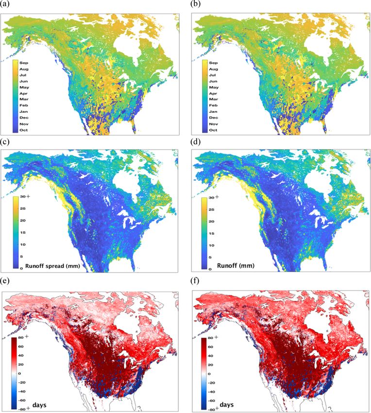
3.4 Uncertainties in the runoff estimation Overall, both Figs. 4 and 11 show the strong influence
of SWE on R over most of North America and, in particu-
Since runoff (R) estimation, in particular, is significantly in- lar, during the snowmelt season. In order to further exam-
fluenced by snow evolution, here we examine the impact of ine this, we explore the difference between average DOY
uncertainty in SWE estimation on the R estimates and their of peak SWE and its spread and average DOY of peak R
uncertainty across North America. Similar to Fig. 4, season- and its spread. Figure 11e shows this date difference of av-
ality of R estimates and their uncertainty are evaluated dur- erage DOY of highest uncertainty (DOY of peak spread in
ing each winter season and over the entire time period and R minus the DOY of peak spread in SWE) and provides a
quantified by computing the average DOY with the highest measure of the spatio-temporal dependence of SWE uncer-
ensemble spread and peak R. Figure 11 shows the average tainty to R uncertainty. Figure 11f shows the date difference
DOY with the highest spread in order to identify the (a) times between the average DOY of highest SWE and highest R,
of high uncertainty in R, (b) average DOY with the peak R, which provides a measure of temporal dependence of high-
(c) highest R ensemble spread, and (d) magnitude of the peak est SWE on the highest R. If this difference is negative, it
R. Variability in the date of the peak R uncertainty and peak likely indicates that SWE is not a primary driver of runoff.
R ranges from June–August in the high latitudes, whereas On the other hand, if this difference is positive, it suggests
at lower latitudes the dates can be outside this range. Sim- that SWE has an influence on the runoff regime. The magni-
ilar to the patterns in Fig. 4c and d, the largest spread and tude of this (positive) difference also provides a measure of
peak R amounts are seen along the northern Pacific coastline the timescale over which they are correlated.
and in eastern Canada along the northern Atlantic coastline We find, from both Fig. 11e and f, that the times of peak R
(excluding the mid-Atlantic and southeastern United States). and uncertainty in peak R occur later in the year than those
Figure 11a and b indicate that the seasonality in the highest of peak SWE and uncertainty in peak SWE over most of
R spread and highest R values is generally matched. In other the domain. Further, the places where we have the negative
words, the largest uncertainty in R occurs at the same time values in both figures are the locations dominated by non-
as the peak R, which is different from the patterns shown in snow R in the lower latitudes. Over the Tundra and Taiga
Fig. 4 where the largest SWE uncertainty is generally during regions, the difference in the average DOY regimes of SWE
the melt season after peak SWE was achieved.
The Cryosphere, 15, 771–791, 2021 https://doi.org/10.5194/tc-15-771-2021R. S. Kim et al.: Snow Ensemble Uncertainty Project (SEUP) 785
Figure 10. Same as Fig. 7 but for forested areas vs. non-forested areas.
and R is about 20–40 d, whereas this lag increases to more 4 Summary and conclusions
than 2 months over the Prairie regions. Over the mountain-
ous terrain, R uncertainty is more closely tied with the SWE This study employs an ensemble modeling approach to quan-
uncertainty (∼ 20 d). tify the spatial and temporal uncertainties in SWE over North
This analysis reconfirms that there is generally explicit America, as estimated by operational LSMs and forcing data.
snow runoff signal during the melt season, and increased Specifically, the study quantifies how uncertainty in SWE
uncertainty in R appears related to uncertainty in preceding varies with key land surface characteristics such as topog-
SWE estimates. Figure 11e and f also provide a measure of raphy, vegetation, and snow climate and evaluates the spatio-
the spatio-temporal utility of SWE measurements when con- temporal influence of significant SWE uncertainty on runoff
sidering the objective of improving R estimation. For exam- estimation. A primary goal of this study is to establish a base-
ple, these figures suggest that SWE estimates approximately line assessment of current global- or continental-scale opera-
60–80 d prior to the peak flow are likely to provide the most tional capabilities and identify potential opportunities where
utility to R estimation over the Prairie regions. Since the improvements or SWE observations could inform both sci-
DOY differences are smaller over the Tundra region, the op- ence and application needs.
timal times for SWE measurements (20 d prior to the peak The SEUP simulated snow estimates are compared against
flow) are less offset relative to the time of peak R. While this a number of spatially distributed reference snow products,
is a preliminary analysis that requires further exploration, it which show a good match over the majority of the modeling
helps to provide insight into the need for improved snow data domain, with an underestimation over the mountainous re-
to improve streamflow estimation. A more detailed examina- gions. The evaluation metrics provide confirmation that the
tion of the influence of SWE–runoff uncertainties, an inves- SEUP ensemble provides a reasonable representation of the
tigation into the utility of SWE observations to reduce SWE snow uncertainty in macroscale snow modeling. Over the
uncertainty, and thereby runoff uncertainty are left for future entire North American domain, the analysis of the SEUP
work. ensemble indicates that the uncertainty in SWE within this
ensemble is driven more by the LSM differences than the
choice of forcing data. This suggests that improvements in
https://doi.org/10.5194/tc-15-771-2021 The Cryosphere, 15, 771–791, 2021You can also read