2010-2015 North American methane emissions, sectoral contributions, and trends: a high-resolution inversion of GOSAT observations of atmospheric ...
←
→
Page content transcription
If your browser does not render page correctly, please read the page content below
Atmos. Chem. Phys., 21, 4339–4356, 2021
https://doi.org/10.5194/acp-21-4339-2021
© Author(s) 2021. This work is distributed under
the Creative Commons Attribution 4.0 License.

2010–2015 North American methane emissions, sectoral
contributions, and trends: a high-resolution inversion of
GOSAT observations of atmospheric methane
Joannes D. Maasakkers1,3 , Daniel J. Jacob1 , Melissa P. Sulprizio1 , Tia R. Scarpelli2 , Hannah Nesser1 ,
Jianxiong Sheng1,4 , Yuzhong Zhang1,5,6,7 , Xiao Lu1 , A. Anthony Bloom8 , Kevin W. Bowman8,9 , John R. Worden8 , and
Robert J. Parker10,11
1 School  of Engineering and Applied Sciences, Harvard University, Cambridge, Massachusetts 02138, USA
2 Department    of Earth and Planetary Sciences, Harvard University, Cambridge, Massachusetts 02138, USA
3 SRON Netherlands Institute for Space Research, Utrecht, the Netherlands
4 Massachusetts Institute of Technology, Cambridge, MA, USA
5 Environmental Defense Fund, Washington, DC, USA
6 School of Engineering, Westlake University, Hangzhou, Zhejiang Province, China
7 Institute of Advanced Technology, Westlake Institute for Advanced Study, Hangzhou, Zhejiang Province, China
8 Jet Propulsion Laboratory, California Institute of Technology, Pasadena, CA, USA
9 Joint Institute for Regional Earth System Science and Engineering, University of California, Los Angeles, CA, USA
10 Earth Observation Science, School of Physics and Astronomy, University of Leicester, Leicester, UK
11 NERC National Centre for Earth Observation, Leicester, UK

Correspondence: Joannes D. Maasakkers (j.d.maasakkers@sron.nl)

Received: 31 August 2020 – Discussion started: 18 September 2020
Revised: 26 December 2020 – Accepted: 7 January 2021 – Published: 22 March 2021

Abstract. We use 2010–2015 Greenhouse Gases Observ-                (28.7 (26.4–36.2) Tg a−1 ). The main discrepancy is for the
ing Satellite (GOSAT) observations of atmospheric methane          oil and gas production sectors, where we find higher emis-
columns over North America in a high-resolution inversion          sions than the GHGI by 35 % and 22 %, respectively. The
of methane emissions, including contributions from differ-         most recent version of the EPA GHGI revises downward its
ent sectors and their trends over the period. The inversion        estimate of emissions from oil production, and we find that
involves an analytical solution to the Bayesian optimization       these are lower than our estimate by a factor of 2. Our best es-
problem for a Gaussian mixture model (GMM) of the emis-            timate of US wetland emissions is 10.2 (5.6–11.1) Tg a−1 , on
sion field with up to 0.5◦ × 0.625◦ resolution in concentrated     the low end of the prior WetCHARTs inventory uncertainty
source regions. The analytical solution provides a closed-         range (14.2 (3.3–32.4) Tg a−1 ), which calls for better under-
form characterization of the information content from the          standing of these emissions. We find an increasing trend in
inversion and facilitates the construction of a large ensem-       US anthropogenic emissions over 2010–2015 of 0.4 % a−1 ,
ble of solutions exploring the effect of different uncertainties   lower than previous GOSAT-based estimates but opposite to
and assumptions in the inverse analysis. Prior estimates for       the decrease reported by the EPA GHGI. Most of this in-
the inversion include a gridded version of the Environmental       crease appears driven by unconventional oil and gas produc-
Protection Agency (EPA) Inventory of US Greenhouse Gas             tion in the eastern US. We also find that oil and gas produc-
Emissions and Sinks (GHGI) and the WetCHARTs model                 tion emissions in Mexico are higher than in the nationally
ensemble for wetlands. Our best estimate for mean 2010–            reported inventory, though there is evidence for a 2010–2015
2015 US anthropogenic emissions is 30.6 (range: 29.4–              decrease in emissions from offshore oil production.
31.3) Tg a−1 , slightly higher than the gridded EPA inventory

Published by Copernicus Publications on behalf of the European Geosciences Union.
4340                                    J. D. Maasakkers et al.: 2010–2015 North American methane emissions and trends

1   Introduction                                                   and Janssens-Maenhout, 2012; Janssens-Maenhout et al.,
                                                                   2019) as a prior estimate, but the EDGAR spatial distribu-
Methane is the second-most important greenhouse gas in             tions have large errors that affect inversion results, and their
terms of radiative forcing (Stocker et al., 2013). Global          interpretation (Maasakkers et al., 2016). Alvarez et al. (2018)
methane concentrations have increased by a factor of 2.5           used surface and aircraft data in oil and gas fields to find
compared to preindustrial times (Hartmann et al., 2013)            emissions from oil and gas production 60 % higher than in
and by 7.1 ppb a−1 since 2007 (with the rate peaking above         the EPA GHGI.
10 ppb a−1 in 2014 and 2015) after a period of stabil-                There has also been substantial debate as to the contri-
ity in the early 2000s (https://www.esrl.noaa.gov/gmd/ccgg/        bution of North American emissions to the rising global
trends_ch4/, last access: 20 December 2020). Major emission        methane trend since 2007. Hausmann et al. (2016) proposed
source sectors include wetlands (the main natural source),         an increase in US gas production as an explanation for the
livestock, the fossil fuel industry, and waste management          2007–2014 methane and ethane concentration trends at the
(Kirschke et al., 2013; Saunois et al., 2020). Individual coun-    Zugspitze mountain site in southern Germany. Turner et al.
tries report their anthropogenic emissions to the United Na-       (2016) found a 2.5 % a−1 increase in US emissions for 2002–
tions Framework Convention on Climate Change (UNFCCC)              2014 on the basis of GOSAT and surface methane data.
using methods prescribed by the Intergovernmental Panel            By contrast, Bruhwiler et al. (2017) found from an ensem-
on Climate Change (IPCC) (United Nations, 1992; IPCC,              ble of inversions using surface and satellite observations
2006). The reports use “bottom-up” methods, where activ-           that North American emissions had been flat for 2000–2012
ity data (e.g., heads of cattle) are combined with emission        and that without an inverse model short-term trends can ap-
factors (e.g., emission per head of cattle) to estimate total      pear to be present in the GOSAT data because of interan-
emissions. US emissions are calculated and reported in this        nual transport variability, choice of background, and the sea-
manner by the Environmental Protection Agency (EPA) in             sonal sampling bias of GOSAT. Sheng et al. (2018a) ana-
its annual Inventory of US Greenhouse Gas Emissions and            lyzed 2010–2016 GOSAT enhancements over North Amer-
Sinks (Greenhouse Gas Inventory, GHGI) (EPA, 2020). Mea-           ica and found a 2.5 ± 1.4 % a−1 increase over the US driven
surements of atmospheric methane, including from satellites,       by oil and gas production and livestock emissions in the Mid-
can be used through inverse modeling to provide an evalua-         west. They found no significant trend over Canada (but large
tion of these emission estimates (Streets et al., 2013; Jacob      year-to-year variation driven by wetlands) and a 0.8 % a−1 –
et al., 2016). Here, we evaluate 2010–2015 North American          1.7 % a−1 decrease in Mexican emissions driven by a de-
emissions by inversion of data from the Greenhouse Gases           crease in livestock. Using 2006–2015 surface and aircraft
Observing Satellite (GOSAT), which measures methane con-           observations over the US and Canada, Lan et al. (2019)
centrations at high precision by solar backscatter in the short-   found a 0.7 ± 0.3 % a−1 increase in total US emissions and
wave infrared (SWIR) (Butz et al., 2011; Buchwitz et al.,          a 3.4 ± 1.4 % a−1 increase in oil and gas emissions based
2015; Kuze et al., 2016). We take the gridded version of the       on stations in Oklahoma, North Dakota, and Texas. They
EPA GHGI (Maasakkers et al., 2016) as a prior estimate for         also reported an increase in the ethane : methane emission
the inversion, enabling us to use the inversion results to eval-   ratio, which could lead to an overestimate of the oil and gas
uate the GHGI and guide improvements in its representation         methane trend as inferred from the ethane trend.
of emission processes.                                                Our inverse analysis of the 2010–2015 GOSAT data over
   Several inverse studies using observations of atmospheric       North America optimizes both mean emissions and their
methane have found higher US emissions than reported               long-term trends at high resolution (up to 50 km). The in-
in bottom-up inventories. Miller et al. (2013) estimated           version uses dynamic boundary conditions from a consistent
methane emissions 50 % higher than the EPA GHGI based on           global inversion of the 2010–2015 GOSAT data previously
2007–2008 surface and aircraft observations. They attributed       reported by Maasakkers et al. (2019). We use an analytical
this difference to fossil fuel extraction. Wecht et al. (2014)     solution to the Bayesian inverse optimization problem (Jacob
estimated 40 % higher livestock emissions using 2004 data          et al., 2016), which provides closed-form characterization of
from the SCanning Imaging Absorption spectroMeter for At-          the information content of the solution and also enables us to
mospheric CHartographY (SCIAMACHY) satellite instru-               perform a range of sensitivity inversions (inversion ensem-
ment (Frankenberg et al., 2006). Turner et al. (2015) found        ble) at no added computational cost. We relate the results
anthropogenic emissions to be 50 % higher than the EPA             from our inversion ensemble to the EPA GHGI emissions in
GHGI by inversion of 2009–2011 GOSAT data, attributing             order to inform knowledge of US emissions, their trends, and
the difference to a combination of oil and gas and livestock       the contributions from different sectors.
emissions. Janardanan et al. (2017) found 28 % higher an-
thropogenic emissions over North America based on 2009–
2012 GOSAT data. All these studies used the global grid-
ded Emission Database for Global Atmospheric Research
(EDGAR) inventory (European Commission, 2011; Olivier

Atmos. Chem. Phys., 21, 4339–4356, 2021                                              https://doi.org/10.5194/acp-21-4339-2021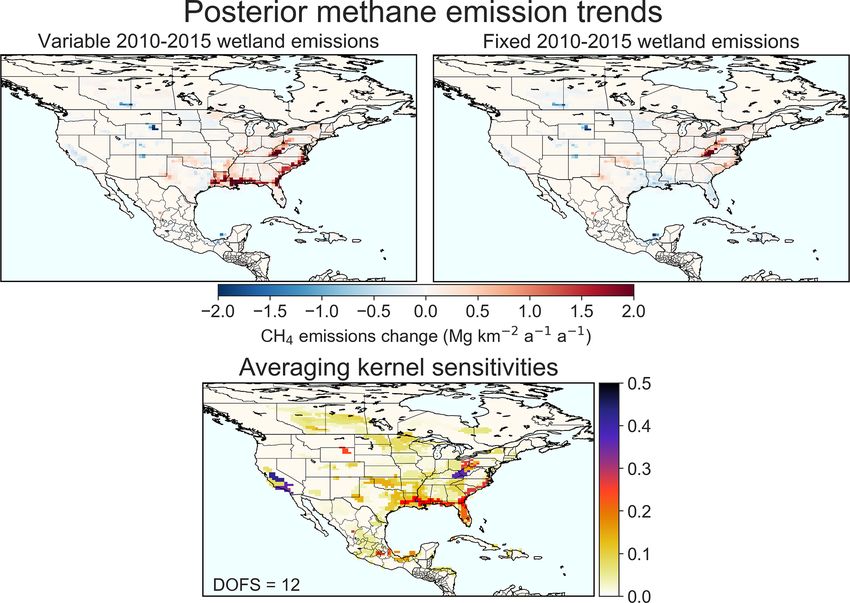
J. D. Maasakkers et al.: 2010–2015 North American methane emissions and trends 4341
2 Data and methods 2.2 Prior estimates
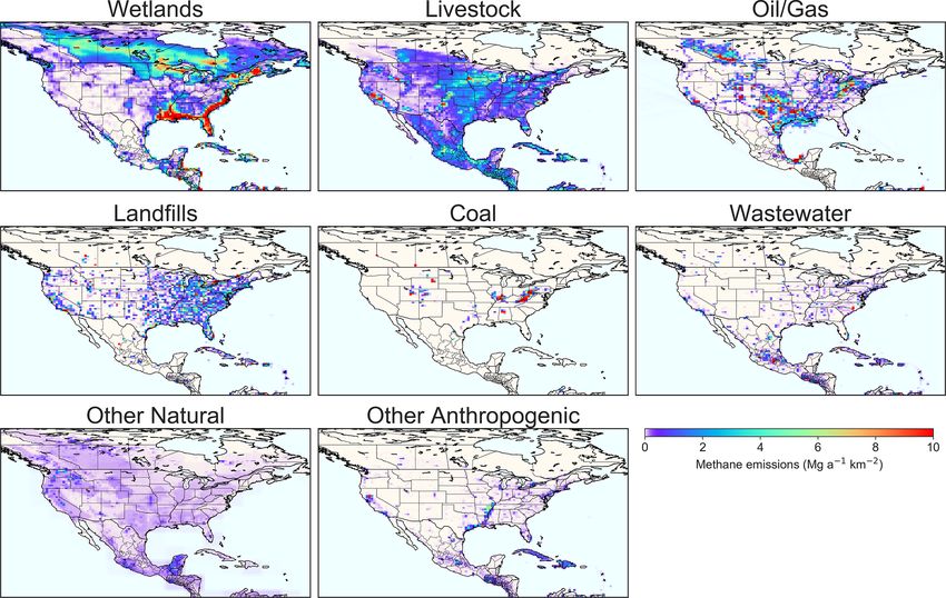
We perform a continental-scale inversion of 2010–2015 Table 1 summarizes our prior emissions estimates, and Fig. 2
GOSAT methane data from the University of Leicester proxy shows their spatial distributions for the major sectors. For all
CH4 retrieval (Parker et al., 2015; ESA CCI GHG project US anthropogenic emissions, including offshore as reported
team, 2018). We use the individual GOSAT observations to to the UNFCCC, we use the spatially disaggregated (grid-
optimize a state vector of mean methane emissions and lin- ded) version of the EPA GHGI (EPA, 2016) for 2012 from
ear emission trends at a spatial resolution of up to 0.5◦ × Maasakkers et al. (2016), with improved spatial allocation of
0.625◦ (≈ 50 km × 50 km). The forward model for the in- emissions and detailed separation of source sectors compared
version is the GEOS-Chem chemical transport model (http: to EDGAR. For oil and gas emissions in Mexico and Canada,
//www.geos-chem.org, last access: 8 March 2021) applied in including offshore, we use gridded versions of the Instituto
nested mode over North America with a spatial resolution Mexicano del Petróleo (IMP) inventory for 2010 (IMP, 2012)
of 0.5◦ × 0.625◦ . The main results presented here are from and the ICF International inventory for 2013 (ICF, 2015), re-
a base inversion with specifications given below. In addition spectively, as reported by Sheng et al. (2017). IMP (2012) oil
to this base inversion, we conducted an ensemble of nine in- and gas emissions for Mexico match the values reported by
versions in which we explored the sensitivity of the results Mexico to the UNFCCC, while ICF (2015) oil and gas emis-
to different assumptions. Specifications for these sensitivity sions for Canada are 43 % higher than the value reported by
inversions are given below and summarized in Sect. 2.5. The Canada (UNFCCC, 2019). The ICF inventory was used as
posterior error covariance matrix from the inversion underes- the basis for the Sheng et al. (2017) gridded emission in-
timates the actual uncertainty in the results because of the as- ventory as it provides a detailed breakdown of sources us-
sumption of fully random observational errors (Jacob et al., ing methodology similar to the EPA GHGI. For other anthro-
2016). Therefore we use the range of results from the in- pogenic emissions in Canada/Mexico and other countries in
version ensemble as a better measure of uncertainty (Heald the domain, we use the EDGAR v4.3.2 global emission in-
et al., 2004). ventory for 2012 (https://edgar.jrc.ec.europa.eu/, last access:
8 March 2021). We separate the general “fuel exploitation”
2.1 GOSAT observations sector reported by EDGAR v4.3.2 into oil and gas and coal
components by using additional information embedded in the
The GOSAT satellite has been observing dry-column
inventory (Greet Maenhout, personal communication, 2018).
methane mixing ratios in the SWIR using the TANSO-FTS
This allows us to use EDGAR coal emissions for Canada and
instrument since April 2009 (Butz et al., 2011). GOSAT in
Mexico. The emissions as given by EDGAR v4.3.2 are asea-
its default mode observes circular pixels of 10 km diameter
sonal. For manure management and rice cultivation we apply
at 13:00 local time, separated by ∼ 250 km along-track and
seasonality as prescribed by Maasakkers et al. (2016) and
cross-track, repeating observation on the same track every
Zhang et al. (2016), respectively. Other anthropogenic emis-
3 d. Additional locations are observed using a target mode.
sions remain aseasonal.
GOSAT methane retrievals have a 24 % success rate, lim-
Natural emissions are dominated by wetlands, for which
ited mainly by cloud cover. Observations have a precision
we use mean monthly emissions from the WetCHARTs v1.0
of 13 ppb and relative bias of 2 ppb compared to the Total
extended ensemble with 0.5◦ ×0.5◦ spatial resolution (Bloom
Carbon Column Observing Network (Buchwitz et al., 2015).
et al., 2017). The ensemble parameters consist of three
There has been no significant spectral degradation of the ob-
global scaling factors (global emissions of 124.5, 166, or
servations over time (Kuze et al., 2016). Figure 1 shows the
207.5 Tg a−1 ), three temperature q10 dependencies (1, 2, or
156 110 retrievals over land used to optimize emissions in
3), and two land cover databases that are combined with pre-
this study (Parker et al., 2015). Each retrieval comes with an
cipitation data to estimate wetland extent (Global Lakes and
estimated retrieval error (11 ppb on average). We use obser-
Wetlands Database, GLWD, from Lehner and Döll, 2004, or
vations over land from January 2010 to December 2015, ex-
GlobCover from Bontemps et al., 2011). Total wetland emis-
cluding data above 60◦ N, for which model errors are large
sions vary month to month and interannually as driven by
(Maasakkers et al., 2019). Most observations (95 365) are
temperature and inundation extent (Bloom et al., 2017). Be-
over the contiguous United States (CONUS). The data are
cause the WetCHARTs ensemble exhibits considerable but
spatially sparse, but this reflects the observing strategy of
uncertain year-to-year variability, we also perform a sensi-
repeated measurements at the same locations in the default
tivity inversion without prior interannual variability in wet-
mode. Thus most observation locations in Fig. 1 have a large
land and other emissions. Daily open-fire emissions are from
number of data points to inform temporal variability and
the Quick Fire Emissions Dataset (QFED) (Darmenov and
trends (Sheng et al., 2018a).
da Silva, 2013), and termite emissions are from Fung et al.
(1991) with a global total of 12 Tg a−1 . We use geological
seepage emissions compiled from the literature on both point
sources (Etiope, 2015; Kvenvolden and Rogers, 2005) and
https://doi.org/10.5194/acp-21-4339-2021 Atmos. Chem. Phys., 21, 4339–4356, 2021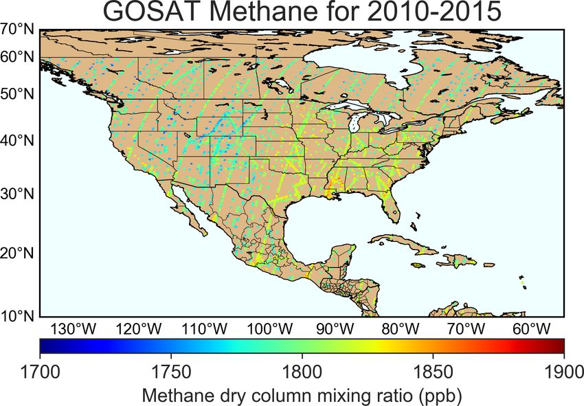
4342                                      J. D. Maasakkers et al.: 2010–2015 North American methane emissions and trends

Figure 1. Average 2010–2015 methane dry-column mixing ratios over North America observed by GOSAT. There are 156 110 individual
observations over land used in the inversion. The GOSAT data have 10 km pixel resolution, but we inflate them here to 0.3◦ × 0.3◦ for
visibility. GOSAT generally takes repeated observations of the same pixels so that most pixels shown here average a number of observations.
The apparent north–south tracks are GOSAT’s default mode observations with a repeat cycle of 3 d, while the off-track data are target mode
observations. GOSAT observations north of 60◦ N are excluded because of their seasonal limitation and uncertainty about the stratospheric
correction.

areal seepage (Kvenvolden and Rogers, 2005; Etiope and                  more abundant data outside that domain) in the global in-
Klusman, 2010) as described in Maasakkers et al. (2019)                 version; but the main consideration here is to avoid bias in
with a global total of 5 Tg a−1 , under the 5.4 Tg a−1 maxi-            boundary conditions that would otherwise affect the North
mum proposed for preindustrial times by Hmiel et al. (2020)             American inversion. Methane chemical and soil sinks are not
based on ice core measurements.                                         optimized in our inversion because they are very slow com-
                                                                        pared to the timescale for ventilation of the North American
2.3    Forward model                                                    domain.
                                                                           Following Maasakkers et al. (2019), we correct the GEOS-
We use the nested version of the GEOS-Chem chemical                     Chem simulation of GOSAT columns for a latitudinally and
transport model v11-01 at 0.5◦ × 0.625◦ resolution over                 seasonally variable background bias likely caused by the ex-
North America as a forward model for the inversion. Ear-                tratropical stratosphere (Bader et al., 2017; Saad et al., 2016;
lier versions of this model for methane were described by               Stanevich, 2018). The bias is common in atmospheric models
Wecht et al. (2014) and Turner et al. (2015). The model                 and caused by excessive meridional transport in the strato-
is driven with MERRA-2 meteorological fields (Bosilovich                sphere (Patra et al., 2011) and in particular in the seasonal
et al., 2016) from the NASA Global Modeling and Assimi-                 polar vortices (Zhang et al., 2021). The latitudinal correc-
lation Office (GMAO). Methane loss from reaction with OH                tion term ξ (ppb) follows a quadratic form as in Turner et al.
and Cl radicals, soil uptake, and stratospheric oxidation is de-        (2015):
scribed in Maasakkers et al. (2019). The simulation is initial-

ized in January 2009 with concentration fields from Turner              ξ = 4.0θ 2 − 1.3θ × 10−3 − 5,                                  (1)
et al. (2015). The 3-hourly boundary conditions at the edges
of the nested domain are from the 4◦ × 5◦ posterior model
simulation of Maasakkers et al. (2019), which provides an               with θ the latitude in degrees. The seasonal bias is corrected
unbiased fit to the global GOSAT data. That posterior sim-              over rolling 8◦ latitudinal bands. A sensitivity inversion with-
ulation includes some information from GOSAT data over                  out the seasonal bias correction is performed as part of the
the North America domain, which were used (along with the               inversion ensemble.

Atmos. Chem. Phys., 21, 4339–4356, 2021                                                    https://doi.org/10.5194/acp-21-4339-2021
J. D. Maasakkers et al.: 2010–2015 North American methane emissions and trends 4343
Table 1. Methane emissions used as prior 2010–2015 estimates.a
Source (Tg a−1 ) CONUS Canada Mexico Otherb
Natural 15.7 15.3 1.4 3.8
Wetlands 14.2 14.4 1.0 3.4
Open fires 0.5 0.3 0.2 0.1
Termites 0.6 0.3 0.1 0.2
Geological seeps 0.5 0.3 0.1 < 0.1
Anthropogenic 28.7 4.5 5.3 5.1
Livestock 9.2 1.0 2.5 1.9
Enteric fermentation 6.7 0.8 2.2 1.9
Manure management 2.5 0.2 0.3 0.1
Oil and natural gas 9.1 2.4 1.5 1.2
Gas production 4.4 1.2 0.1
Oil production 2.3 0.5 1.2
Gas transmission 1.1 0.3 < 0.1
Gas processing 0.9 0.3 0.1
Gas distribution 0.5 < 0.1 < 0.1
Landfills 5.8 0.7 0.4 0.6
Coal mining 2.9 0.1 < 0.1 < 0.1
Wastewater 0.7 0.2 0.7 0.7
Rice cultivation 0.5 < 0.1 < 0.1 0.2
Other anthropogenicc 0.5 0.1 0.2 0.4
Total source 44.5 19.8 6.7 8.9
a CONUS anthropogenic emissions are from the EPA GHGI for 2012 as spatially disaggregated
by Maasakkers et al. (2016). Oil and gas emissions from Canada (2013) and Mexico (2010) are
from ICF (2015) and IMP (2012), respectively, spatially disaggregated by Sheng et al. (2017).
Other anthropogenic emissions are from EDGAR v4.3.2 for 2012
(https://edgar.jrc.ec.europa.eu/, last access: 8 March 2021, European Commission, 2011).
Wetlands and open-fire emissions are mean values for 2010–2015 from the WetCHARTs
ensemble (Bloom et al., 2017) and QFED (Darmenov and da Silva, 2013); termite emissions are
from Fung et al. (1991). Seepage emissions are as described in Maasakkers et al. (2019). The
soil sink is 3.6 Tg a−1 for the inversion domain (Fung et al., 1991) and is not optimized in the
inversion. All values in the table are rounded to one decimal.
b Within the inversion domain shown in Fig. 1 (10–70◦ N, 140–40◦ W) containing parts of
Central and South America.
c Including fossil fuel combustion, industrial processes, agricultural field burning, and
composting.
2.4 State vector for the inversion and error covariances gregation of regions with weak or homogeneous emissions
while preserving high resolution for concentrated emissions.
Although we could technically carry out the inversion of the Each 0.5◦ × 0.625◦ grid cell is represented by a unique com-
GOSAT data at the 0.5◦ × 0.625◦ resolution of the GEOS- bination of the Gaussians so that the optimization of x can be
Chem simulation, the data do not have sufficient informa- mapped to the 0.5◦ ×0.625◦ grid. For more details see Turner
tion to constrain emissions on that grid, and doing so would and Jacob (2015).
incur a large smoothing error (Wecht et al., 2014). We use Prior emission error variances are defined for each Gaus-
instead a 600-element Gaussian mixture model (GMM) as sian on the basis of its spatial distribution and the contribu-
described by Turner and Jacob (2015) to optimally define the tions from different sectors. Emission errors for individual
emission patterns that can be usefully constrained by the in- anthropogenic sectors are estimated using the error curves
version. Each of the 600 Gaussian functions in the GMM is from Maasakkers et al. (2016). The error standard deviation
defined by an emission amplitude, mean location, and spread σ for a given source sector and Gaussian is given by
(standard deviation). These parameters are optimized using σ = (α0 exp(−kα (L − L0 )) + αN ) E, (2)
a similarity vector on the 0.5◦ × 0.625◦ grid that takes into
account latitude, longitude, and the prior patterns of different where α0 , kα , and αN are source-sector-specific error coeffi-
source sectors. The state vector x for the inversion with di- cients from Maasakkers et al. (2016); L is the effective spa-
mension n = 2 × 600 consists of scaling factors adjusting the tial resolution (length scale) of the Gaussian defined by the
amplitudes of the Gaussians in the GMM and their 2010– number of 0.5◦ × 0.625◦ grid cells it represents; L0 = 0.1◦
2015 linear trends. This approach allows for effective ag- is the native resolution of the prior inventory; and E is the
https://doi.org/10.5194/acp-21-4339-2021 Atmos. Chem. Phys., 21, 4339–4356, 20214344 J. D. Maasakkers et al.: 2010–2015 North American methane emissions and trends Figure 2. Mean prior estimates of methane emissions for 2010–2015. National totals, subsector breakdowns, and references are in Table 1. sum of emissions from the source sector within the Gaussian 2019). We also perform sensitivity inversions with changes (sum of emissions from 0.5◦ × 0.625◦ grid cells weighted by of 2.5 % a−1 and 10 % a−1 as the prior error standard devi- their contributions to the Gaussian). Maasakkers et al. (2016) ation. Off-diagonal elements of SA are assumed to be 0 be- also include a displacement error related to uncertainty in cause Maasakkers et al. (2016) found no spatial error corre- source location, but this error is negligible at our resolu- lation for the gridded EPA inventory; this may be an under- tion. For wetland emissions, we use the standard deviation estimate for wetland emissions (Bloom et al., 2017). in monthly estimates of the 18 WetCHARTs v1.0 extended Our calculation of SA leads to different error variances for ensemble members averaged over the Gaussian; the result- each grid cell. To assess the impact of that choice, we also ing error standard deviation is 78 % on average. For the other perform a sensitivity inversion using the mean error variance natural emissions we assume 100 % error at the 0.5◦ ×0.625◦ for all the Gaussians. The base inversion assumes normal model resolution. errors, but we also perform a sensitivity inversion assum- The error variances for all sectors contributing to a given ing log-normal emission errors following the Levenberg– Gaussian are added in quadrature to obtain the correspond- Marquardt method as described in Maasakkers et al. (2019). ing diagonal element of the prior error covariance matrix SA . We use the residual error method (Heald et al., 2004) Error variances for a given Gaussian are capped at 50 % in to construct the diagonal of the observational error covari- the base inversion, and we also perform a sensitivity inver- ance matrix SO . The mean 2010–2015 difference between sion without this cap. The mean relative error standard de- GOSAT and the prior model (before seasonal correction) for viation is 37 % in the base inversion. The 50 % cap mainly each 0.5◦ × 0.625◦ grid cell is assumed to be due to errors in affects Gaussians dominated by wetland emissions. For the emissions, to be corrected by the inversion. After subtracting 2010–2015 emission trends associated with each Gaussian, this mean difference, the residual standard deviation is taken the prior estimate is set to 0, and the prior error standard as an estimate of the observational error standard deviation, deviation is a 5 % change per year, in line with uncertain- including contributions from instrument, representation, and ties in trend estimates for North America (Turner et al., forward model errors. If this estimate is less than the reported 2016; Bruhwiler et al., 2017; Sheng et al., 2018a; Lan et al., instrument error standard deviation (Parker et al., 2015), we Atmos. Chem. Phys., 21, 4339–4356, 2021 https://doi.org/10.5194/acp-21-4339-2021
J. D. Maasakkers et al.: 2010–2015 North American methane emissions and trends 4345
use the latter instead (17 % of observations). If it is less than The trace of A gives the degrees of freedom for signal
10 ppb we reset it to 10 ppb (6 % of observations). The result- (DOFSs), which measures the number of independent pieces
ing average observational error standard deviation is 14 ppb. of information on the state vector that can be obtained from
Off-diagonal terms of SO are assumed to be 0 for lack of bet- the inversion. The diagonal elements of A (averaging kernel
ter information, but in fact some transport error correlation sensitivities) measure the degree to which the inversion can
would be expected in the forward model. We account for this constrain the true values of the corresponding state vector el-
error correlation with a regularization term γ in the inversion ements (1 = perfectly, 0 = not at all). We use these measures
(Sect. 2.5). of information in our presentation of results.
The analytical solution to the inverse problem requires ex-
2.5 Inversion procedure plicit construction of the Jacobian matrix. We perform this
construction column by column by perturbing individually
We perform an analytical inversion minimizing the Bayesian the 1200 elements of the state vector and conducting the cor-
cost function J (x) assuming normal errors (Rodgers, 2000): responding GEOS-Chem simulations for the 2010–2015 ob-
servation record. This is readily done as a massively parallel
J (x) = (x − xA )T SA −1 (x − xA ) + γ (y − F (x))T SO −1
calculation. Aside from enabling closed-form characteriza-
(y − F (x)) , (3) tion of the information content from the inversion, a major
advantage of the analytical solution once the Jacobian ma-
where x is the state vector to be optimized, consisting of
trix has been constructed is that the sensitivity of the solu-
600 Gaussians for which we optimize both scaling factors
tion to various assumptions and choices made in the inver-
for mean emissions and absolute linear emission trends, for a
sion approach can be immediately obtained. In addition to
total of 1200 state vector elements; xA is the prior state vec-
our base inversion, we generate in this manner an ensem-
tor; SA is the prior error covariance matrix (Sect. 2.4); SO is
ble of nine sensitivity inversions introduced in the text above
the observational error covariance matrix (Sect. 2.4); γ is a
and for which the ensemble of solutions gives a better mea-
regularization factor to account for the lack of non-diagonal
sure of posterior error than can be obtained from b S (Heald
terms in SO and hence prevent overfitting, and it plays a sim-
et al., 2004). To summarize, these sensitivity inversions in-
ilar role as the regularization parameter in Tikhonov methods
clude (1) using a prior estimate with no interannual variabil-
(Brasseur and Jacob, 2017) and reflects our inability to pre-
ity (2012 values) for wetland and biomass burning emissions
cisely quantify error statistics in the Bayesian method. Here
and for the soil sink, (2) not using a seasonal correction to the
we find that γ = 0.5 provides the best balance of fitting the
GOSAT–model mismatch, (3) using emission error variances
prior and observational terms in the cost function, following
without the 50 % cap, (4) using the average-emission and
the L-curve approach of Hansen (1999). The value is higher
absolute-trend error variances (37 % and 2.3 Mg a−2 km−2 ,
than γ = 0.05 used in the global inversion of Maasakkers
respectively) for each Gaussian, (5, 6) assuming error prior
et al. (2019) at 4◦ × 5◦ resolution because here we have a
standard deviations for the 2010–2015 trend of 2.5 % and
smaller number of observations per state vector element. We
10 % annual change in emissions (instead of 5 %), (7) as-
also conduct sensitivity inversions with γ = 0.1 and γ = 1.
suming log-normal prior emission errors, and (8, 9) using
The GEOS-Chem forward model (y = F (x)) as imple-
regularization factors for the cost function γ = 0.1 and γ = 1
mented here is strictly linear in its relationship between
(instead of γ = 0.5).
methane column concentrations (y) and the state vector of
emissions (x). It can be expressed as F (x) = Kx + c, where
K = ∂y/∂x is the Jacobian matrix, and c is an initialization
3 Results and discussion
constant. This allows the optimal posterior solution bx, which
minimizes the cost function J (x), to be obtained analytically
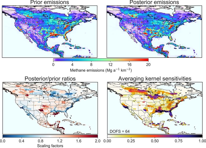
Figure 3 shows mean prior and posterior emissions for 2010–
as
2015, the ratio between the two, and the inversion’s averag-
SO −1 ing kernel sensitivities (Eq. 6). The averaging kernel sensi-
T T
x = xA + SA K KSA K +
b (y − KxA ) (4) tivities identify regions where the GOSAT observations pro-
γ
vide significant information on emissions. These are regions
S:
with posterior error correlation matrix b with a high density of observations and/or high absolute un-
−1 certainties in the prior emissions. For example, we achieve
S = γ KT SO −1 K + SA −1
b . (5) good constraints on emissions in central Canada, much of
the eastern and central US, California, and southeastern Mex-
The information content from the inversion can then be ob- ico. Other regions receive little information from the obser-
tained from the averaging kernel matrix (A = ∂b x/∂x), which vations, which explains a lack of departure from the prior
gives the sensitivity of the solution to the true state: estimate.
The posterior emissions when implemented in GEOS-
SSA −1 .
A = I −b (6) Chem reduce the mean squared difference with GOSAT ob-
https://doi.org/10.5194/acp-21-4339-2021 Atmos. Chem. Phys., 21, 4339–4356, 20214346 J. D. Maasakkers et al.: 2010–2015 North American methane emissions and trends
Figure 3. Mean 2010–2015 posterior methane emissions projected from the 600-member Gaussian mixture to the 0.5◦ × 0.625◦ model grid
and comparison to the prior estimate. Results are from the base inversion. The bottom right panel shows the averaging kernel sensitivities
projected to the model grid (diagonal elements of the averaging kernel matrix). The trace of the averaging kernel matrix, i.e., the degrees
of freedom for signal (DOFSs), is given inset. It represents the number of independent pieces of information that can be constrained by the
inversion.
servations by 3.5 %. This overall reduction in error is small time-averaged GEOS-Chem and NOAA data increases from
because random errors in individual observations are large r 2 = 0.58 with the prior emissions to r 2 = 0.81 with the pos-
and because the background is already captured well in the terior emissions, representing an improvement in our ability
prior simulation through the optimized boundary conditions. to fit observed patterns.
The main improvements are found over areas where the aver-
aging kernels are large (Fig. 3). For data with averaging ker- 3.1 Mean 2010–2015 emissions
nel sensitivities greater than 0.1, the mean squared difference
is reduced by 6.1 %, and the correlation increases from 0.62 Although the inversion yields little change in total emissions
to 0.64. We independently evaluated the posterior estimate for the continental domain, there are large regional changes,
by comparison to in situ methane concentrations from sur- as shown in Fig. 3. We find higher emissions over the south-
face sites reported in the GLOBALVIEWplus CH4 ObsPack central and eastern US and lower emissions in California
v1.0 data product compiled by the NOAA Global Monitor- compared to the gridded EPA inventory. The WetCHARTs
ing Laboratory (Cooperative Global Atmospheric Data Inte- inventory overestimates wetland emissions, including along
gration Project, 2019). Compared to the prior simulation (re- the Gulf Coast and East Coast of the US, the upper Mid-
duced major axis (RMA) slope = 0.69, r 2 = 0.39), the poste- west, and Canada. Emissions in eastern Mexico are higher
rior simulation (RMA slope = 0.69, r 2 = 0.45) does not de- than inferred from the IMP (2012) inventory. The inversion
grade the comparison with these data and improves the cor- also shows large relative increases from oil production off
relation. The spatial coefficient of determination between the the Louisiana coast and from wetlands or livestock in west-
ern Montana, but the associated emissions are low. The large-
Atmos. Chem. Phys., 21, 4339–4356, 2021 https://doi.org/10.5194/acp-21-4339-2021J. D. Maasakkers et al.: 2010–2015 North American methane emissions and trends 4347 scale correction patterns revealed by the inversion are simi- lar to those of the coarse (4◦ × 5◦ ) global inversion reported by Maasakkers et al. (2019), which used the same prior es- timates, but the higher resolution of the inversion allows us much more detail here. Figure 4 shows the attribution of the inversion results to individual source sectors for CONUS, Canada, and Mexico. This attribution was made by applying the correction fac- tors to the sectoral emissions in each grid cell, assuming that the relative contributions of individual sectors to emissions in that grid cell are correct in the prior emission inventory (this does not assume that the total prior distribution of sec- toral emissions is correct). Vertical bars show the range of results from the inversion ensemble. A narrow uncertainty range does not necessarily reflect confidence in the inversion results. For small source sectors, it may also be due to in- sufficient information from the observations so that the opti- mization is unable to depart from the prior estimate. This can be determined using the averaging kernel sensitivities, as is done below for the US (see Table 2). The largest decrease is for US wetland emissions, mostly contributed by the Gulf Coast and East Coast (Fig. 2). Such an overestimate in the mean of the WetCHARTs wetland in- ventory ensemble was previously identified in an inversion of aircraft observations over the southeast US (Sheng et al., 2018b). It may be related to the low organic carbon content of the soil, the difficulty of distinguishing freshwater and salt- water wetlands, uncertainties in anaerobic CH4 : CO2 respi- ration rates, and the accounting of partial wetland land cover areas (Holmquist et al., 2018; Lehner and Döll, 2004; Bloom et al., 2017). We also find an overestimate of wetland emis- sions in (mainly eastern) Canada. The large uncertainty range is driven by the inversion ensemble member without seasonal correction. Based on the root mean square error and spatial correlation, our inversion results are most consistent with the WetCHARTs ensemble members that use GlobCover wet- land extent, a q10 = 2 value for the factor increase in the CH4 : CO2 emission ratio per 10 K temperature increase (a critical quantity for determining the sensitivity of wetland CH4 production to temperature; Yvon-Durocher et al., 2014; Bloom et al., 2016), and global scaling at the low end or middle of the range (global wetland emission range: 125– 166 Tg a−1 ). A value of q10 = 2 is approximately equivalent to the average CH4 : CO2 temperature sensitivity reported by Figure 4. Mean 2010–2015 methane emissions per source sector Yvon-Durocher et al. (2014) based on meta-analyses, which for the contiguous US (CONUS), Canada, and Mexico. Values are indicates that anaerobic CH4 respiration is substantially more shown for the prior estimates (Table 1) and for the posterior esti- sensitive to temperature relative to overall CO2 respiration mates after inversion of GOSAT data. Vertical bars show the ranges rates. Sheng et al. (2018b) also found their inversion results of results from the inversion ensemble. to be most consistent with GlobCover but also favored no CH4 : CO2 temperature dependence (q10 = 1). Their obser- vations were much more limited in space and time (August– and gas emissions (+22 (−24–42) %). Uncertainty ranges in September 2013). correcting individual sectors are large for Mexico because Figure 4 also shows some significant sectoral corrections of the extensive spatial overlap between sectors (Fig. 2). for anthropogenic emissions in the US and Mexico. Over Most of the oil and gas correction is for coastal and off- Mexico we find higher livestock (+13 (5–24) %) and oil shore oil production (Fig. 3). We also find 56 (31–120) % https://doi.org/10.5194/acp-21-4339-2021 Atmos. Chem. Phys., 21, 4339–4356, 2021
4348                                        J. D. Maasakkers et al.: 2010–2015 North American methane emissions and trends

Table 2. Mean 2010–2015 methane emissions in the contiguous US (CONUS).

                         Source (Tg a−1 )                          Prior estimatea         Posterior estimateb           Sensitivityc
                         Natural                                                 15.7           11.8 (7.1–12.7)                   0.63
                            Wetlands                                             14.2           10.2 (5.6–11.1)                   0.71
                            Open fires                                            0.5             0.4 (0.4–0.5)                   0.13
                            Termites                                              0.6             0.6 (0.6–0.6)                  −0.02
                            Geological seeps                                      0.5             0.5 (0.5–0.5)                   0.06
                         Anthropogenic                                           28.7          30.6 (29.4–31.3)                    0.53
                           Livestock
                               Enteric fermentation                                6.7              6.9 (6.3–7.0)                  0.16
                               Manure management                                   2.5              2.5 (2.1–2.5)                  0.22
                           Oil and natural gas
                               Gas production                                      4.4              5.4 (4.9–5.9)                  0.28
                               Oil production                                      2.3              3.1 (2.7–3.6)                  0.53
                               Gas transmission                                    1.1              1.1 (1.1–1.2)                  0.03
                               Gas processing                                      0.9              1.1 (1.0–1.2)                  0.41
                               Gas distribution                                    0.5              0.4 (0.4–0.4)                  0.35
                           Landfills
                               Municipal                                           5.2              5.0 (4.7–5.0)                  0.26
                               Industrial                                          0.6              0.5 (0.5–0.5)                  0.13
                           Coal mining
                               Underground                                         2.2              2.4 (2.3–2.5)                  0.22
                               Surface                                             0.5              0.5 (0.4–0.5)                  0.30
                               Abandoned                                           0.2              0.3 (0.3–0.3)                  0.10
                           Wastewater
                               Municipal                                           0.5              0.4 (0.4–0.4)                  0.09
                               Industrial                                          0.2              0.2 (0.1–0.2)                  0.16
                           Rice cultivation                                        0.5              0.4 (0.3–0.5)                  0.28
                           Other anthropogenicd                                    0.5              0.4 (0.4–0.5)                  0.05
                         Total source                                            44.5          42.4 (37.0–42.9)                    0.64
                       a The prior estimates include the 2012 EPA GHGI emissions (EPA, 2016) and the 2010–2015 mean of the
                       WetCHARTs inventory ensemble for wetlands (Bloom et al., 2017).
                       b Posterior estimates from our base inversion, with the range from the inversion ensemble in parentheses.
                       c Sensitivity of the posterior estimate to the observations as diagnosed from the averaging kernel matrix,
                       ranging from 0 (no sensitivity, posterior equal to prior) to 1 (full sensitivity, posterior solely determined by the
                       observations). For example, a sensitivity of 0.64 means that 64 % of the posterior estimate is constrained by the
                       observations, and 36 % is constrained by the prior. Averaging kernel sensitivities can statistically be negative in
                       case of error overlap with other sources. The small negative value here is insignificant.
                       d Including fossil fuel combustion, industrial processes, agricultural field burning, and composting.

higher emissions over Mexico City, which is optimized by                             ble also includes the averaging kernel sensitivity ai,i from
a single Gaussian covering five grid cells. The difference is                        the inversion for each sector and subsector i, which we esti-
attributed to wastewater based on the EDGAR spatial pat-                             mate by summing emissions from sector or subsector i for all
terns. Compared to EDGAR v4.3.2, a recent gridded in-                                0.5◦ × 0.625◦ grid cells over the CONUS into one state vec-
ventory for Mexico (Scarpelli et al., 2020) and the Mexico                           tor element using a summation matrix (Calisesi et al., 2005;
City Secretariat of Environment (SEDEMA, 2018) air qual-                             Maasakkers et al., 2019). The summation matrix (W) weighs
ity emission inventory predict lower emissions from wastew-                          the relative contribution wi,k of sector or subsector i to the
ater (68 versus 259 Gg a−1 in the Secretaría del Medio Am-                           total emission in Gaussian k in the prior inventory:
biente (SEDEMA; Mexico City Secretariat of Environment)
inventory) but much higher landfill emissions (222 ver-                              Asub = WAW∗                                                   (7)
sus 1 Gg a−1 ), indicating that our higher emission estimate                         Sd      b T
                                                                                      sub = WSW .                                                  (8)
may be related to landfill emissions being misallocated in
EDGAR v4.3.2.                                                                                                 −1
   Inversion results for the US mapped onto the detailed                             Here W∗ = WT WWT               is the generalized pseudo-
source sectors and subsectors from the gridded EPA inven-                            inverse of W, and Asub (with diagonal elements ai,i ) and
tory (Maasakkers et al., 2016) are given in Table 2. The ta-                         Sdsub are the averaging kernel matrix and posterior error co-

Atmos. Chem. Phys., 21, 4339–4356, 2021                                                                       https://doi.org/10.5194/acp-21-4339-2021
J. D. Maasakkers et al.: 2010–2015 North American methane emissions and trends 4349
variance matrix mapped to the different subsectors; ai,i = 1
means that the inversion can fully constrain the national to-
tal for that emission category, independent of the prior es-
timate, while ai,i = 0 means that the inversion provides no
information, and the estimate cannot depart from the prior.
The off-diagonal elements of Sd sub measure the error corre-
lation in the posterior solution for different subsectors, and
this is important to diagnose whether we can optimize differ-
ent subsectors independently. The diagonal elements of Sd sub
estimate the error variance in the posterior solution for indi-
vidual subsectors, but that estimate is too small because it as-
sumes that the observations are independent and identically
distributed (IID condition) (Brasseur and Jacob, 2017). We
prefer to estimate the error in the posterior solution from the Figure 5. Methane emissions from the oil and gas sector in the con-
results of the inversion ensemble, as shown in Table 2. tiguous US (CONUS) in 20212. The figure shows the original EPA
The averaging kernel sensitivities for individual sectors GHGI estimates for 2012 used as a prior in the inversion (EPA,
and subsectors in Table 2 vary based on the uncertainty in the 2016), the updated EPA GHGI estimates for 2012 based on revised
prior emission estimates and the GOSAT observation den- methodology (EPA, 2020), and the posterior results from the inver-
sity in the regions of emissions. Posterior wetland emissions sion. Horizontal bars give the ranges of the inversion ensemble.
(ai,i = 0.70) are 70 % informed by the observations (30 %
by the prior) because the prior uncertainty is large. We also
calculate ai,i for the sum of US anthropogenic emission cate- and gas subsectors, as shown in Fig. 5. Gas production emis-
gories and find emissions are 53 % informed by the observa- sions in 2012 are lower by 19 % in the updated GHGI be-
tions, with less information for individual sectors and subsec- cause of a downward correction to emissions from gathering
tors. Emissions from oil and gas production are particularly and boosting stations. Oil production emissions in 2012 are
well informed (28 %–52 %) because they are large and have 30 % lower in the updated EPA GHGI because of previous
relatively little spatial overlap with other sectors. faulty double-counting of wells. Our correction factor from
Our posterior estimate for the mean 2010–2015 CONUS the inversion increases oil production emissions by a factor
anthropogenic source is 30.6 (29.4–31.3) Tg a−1 , where the of 1.9 (1.7–2.3) and natural gas production emissions by a
best estimate is from the base inversion, and the range is factor of 1.5 (1.4–1.6) relative to the updated 2012 GHGI
from the inversion ensemble. The 2012 emission total from from the EPA (2020). The updated GHGI emissions from
the EPA GHGI (EPA, 2016) used as a prior estimate in our natural gas processing in 2012 are 55 % lower than previ-
inversion is 28.7 Tg a−1 , with an uncertainty range of 26.4– ously reported, but our inversion finds them to be higher. Our
36.2. We find limited posterior error correlation (r = 0.33) correction factor from the inversion increases gas processing
between the posterior anthropogenic and natural emission to- emissions by a factor of 2.9 (2.6–3.1) relative to the updated
tals. Examining the contributions from different sectors, our GHGI.
best posterior estimates for landfills and livestock are within
5 % of the GHGI, and coal emissions are 6 % higher. Oil and 3.2 2010–2015 emission trends
gas emissions total 11.1 Tg a−1 in our base inversion, 22 (12–
32) % higher than the GHGI, and are driven by oil and gas Figure 6 shows linear emission trends for 2010–2015 opti-
production as seen for example in Texas, Oklahoma, and off- mized by the base inversion (top left panel) and the sensi-
shore in the Gulf of Mexico. Our national estimates for the tivity inversion, including no interannual variability in prior
emissions from oil and gas production are 3.1 (2.7–3.6) and estimates for wetlands and open fires (top right panel). The
5.4 (4.9–5.9) Tg a−1 , respectively, as compared to 2.3 and base inversion shows a trend of increasing emissions from
4.4 Tg a−1 in the GHGI. The posterior error covariance be- US wetlands, but this is relative to the prior WetCHARTs es-
tween wetland emissions and both oil production (r = 0.02) timate of interannual variability in wetland emissions, which
and gas production (r = 0.04) are low, showing that this in- vary from 31 Tg in 2015 to 36 Tg in 2010. Due to the spar-
crease is independent of the large decrease in wetland emis- sity of independent constraints, the WetCHARTs interan-
sions. nual variations have not been extensively evaluated (Bloom
Our scaling factors to the EPA GHGI are for the 2012 et al., 2017); therefore we have little confidence in these
emissions as reported by the EPA (2016) and used in the in- year-to-year emission changes. The sensitivity inversion in-
version as prior estimates. More recently, the EPA (2020) up- cluding no prior interannual variability for wetlands shows
dated its methodology for estimating emissions and applied no large trends in US wetland emissions. Both inversions
it to a reanalysis of emissions from previous years, including show similar results for the emission trends in anthropogenic
2012. Changes for 2012 emissions are important for some oil source regions. We find an increase in total anthropogenic
https://doi.org/10.5194/acp-21-4339-2021 Atmos. Chem. Phys., 21, 4339–4356, 20214350 J. D. Maasakkers et al.: 2010–2015 North American methane emissions and trends CONUS emissions of 0.14 Tg a−1 a−1 (0.4 % a−1 ) over the decreased, and efforts have been made to reduce emissions 2010–2015 period. This anthropogenic trend is much lower (Natural Resources Canada, 2020). than the 2.8 ± 0.3 % a−1 increase reported for 2010–2014 by Turner et al. (2016) and more in line with the 2006–2015 3.3 Comparison with other evaluations of the EPA trend of 0.7 ± 0.3 % a−1 in total US emissions estimated by inventory Lan et al. (2019). The GHGI (EPA, 2020) reports a 0.35 Tg a−1 a−1 decrease A number of studies using atmospheric measurements over in anthropogenic US emissions from 2010 to 2015, at odds the US have previously compared their findings to the grid- with our result. The decrease in the GHGI is mainly driven by ded version of the EPA GHGI reported by Maasakkers et al. decreasing emissions from landfills (−0.10 Tg a−1 a−1 ) and (2016) and used as a prior estimate in our inversion. Based on coal mining (−0.17 Tg a−1 a−1 ). We find small decreases in an upscaling of facility-level measurements and aircraft data, the western US that may be related to decreases in emis- Alvarez et al. (2018) estimated 2015 US oil and gas emis- sions from landfills or coal mines (Wyoming). On the na- sions of 13 (11–15) Tg a−1 , consistent with our posterior es- tional scale, however, the inversion does not detect decreas- timate of 11.4 (10.3–12.2) Tg a−1 for 2015 (posterior mean ing emissions from landfills or coal mining. 2010–2015 emissions plus trend) and much higher than the For total oil and gas emissions we find a US trend of 0.4 7.3 Tg a−1 national total from the latest GHGI (EPA, 2020). (0–1) % a−1 for 2010–2015, smaller than the 3.4 ± 1.4 % a−1 Similar to our subsector attribution, Alvarez et al. (2018) find increase reported by Lan et al. (2019) for 2006–2015. The the largest difference with the GHGI for the production sub- discrepancy may be explained by the different time periods sector (factor of 2), which they attribute to the GHGI emis- and the fact that the Lan et al. (2019) oil and gas trend is sions not accounting for emissions from abnormal operating mainly determined by stations in Oklahoma, North Dakota, conditions. While Alvarez et al. (2018) did not distinguish and Texas. Most of our increase is driven by the Marcel- between oil and gas production, our results point at a much lus Shale area in the northeast US, amounting to 130 (20– larger relative discrepancy with the GHGI for oil production 190) Gg a−1 a−1 . This area covering Pennsylvania, Ohio, and emissions than natural gas production emissions. West Virginia has seen a large increase in natural gas pro- In an inversion of data from two tower networks and one duction driven by unconventional drilling. Natural gas pro- aircraft campaign, Cui et al. (2019) found 2014–2016 Cali- duction in the area increased by a factor of 7.8 between 2010 fornia methane emissions to be 2.05 ± 0.26 Tg a−1 . Our pos- and 2015, contributing 22 % of US natural gas production in terior estimate of 2015 California emissions is 1.6 (0.8– 2015 (EIA, 2020a). If the 130 (20–190) Gg a−1 a−1 increase 1.7) Tg a−1 , representing a significant decrease from the prior is entirely due to gas production, it would only amount to estimate of 2.3 Tg a−1 . This is due to our large reduction in 15 (2–21) % a−1 relative to the mean posterior gas produc- mean 2010–2015 emissions in the Los Angeles Basin. This tion emissions in the area (0.89 Tg a−1 ), indicating that the reduction may be overestimated because of the coarseness leakage rate did decrease over the time period. The latest of model CO2 used in the proxy retrieval, underestimating GHGI shows a national 60 Gg a−1 a−1 decrease in natural CO2 over Los Angeles (Turner et al., 2015). Using aircraft gas production emissions over the 2010–2015 period (EPA, measurements, Ren et al. (2019) found 70 % higher oil and 2020), mainly due to decreasing onshore production and ex- gas production emissions in the Marcellus Shale (Pennsylva- ploration emissions and partly offset by increasing gathering nia and West Virginia) in 2015 compared to the 2012 grid- and boosting emissions. For onshore production emissions, ded EPA inventory, which they attribute to an increase in the GHGI primarily estimates emissions on the basis of the production. We find a 2010–2015 increase in emissions for number of wells rather than by production rate, and this may that region, as discussed above, but 2015 emissions are still underestimate the trend in the Marcellus Shale as the num- only 22 % higher than the GHGI. Based on surface obser- ber of wells only increased by 13 % over 2010–2015 (EIA, vations in the Uintah Basin in Utah, Foster et al. (2017) 2020b) despite the large increase in production. The inver- found good agreement with basin-wide emissions from Kar- sion suggests additional increases over production regions in ion et al. (2013) and found the gridded EPA inventory to be Texas (Permian Basin) and Oklahoma. The Permian Basin 45 % lower after adjusting emissions based on 2015 produc- has seen a large increase in production after 2015 (beyond tion data. Most of the emissions in the Uintah Basin are con- the time span of our inversion) and is currently the largest centrated in one of our grid cells, and that cell is optimized oil-producing basin in the US (Zhang et al., 2020). individually in our inversion with good constraints (Fig. 3), GOSAT provides little information over Canada and Mex- finding 2015 posterior emissions that are 37(12–66) % higher ico when it comes to trends. There are signs that oil and gas than the prior and no significant 2010–2015 trend. production emissions in both Alberta (Canada) and offshore Based on aircraft data, Plant et al. (2019) found anthro- in the Gulf of Mexico are decreasing, and the latter may be pogenic urban methane emissions that were higher than the driven by decreasing oil production (Zhang et al., 2019). In gridded EPA inventory over five cities on the US East Coast Canada, gas production has been stable, while oil production by a factor of 2. We find no such difference, but evaluat- from oil sands has increased, but the number of wells has ing urban emissions along the East Coast is difficult because Atmos. Chem. Phys., 21, 4339–4356, 2021 https://doi.org/10.5194/acp-21-4339-2021
J. D. Maasakkers et al.: 2010–2015 North American methane emissions and trends                                                            4351

Figure 6. Methane emission trends for 2010–2015 in North America. The top panels show the posterior estimates from the inversion of
GOSAT satellite data, allowing for 2010–2015 interannual variability in the prior estimates for wetlands and open fires (base inversion, left)
and not allowing for that prior interannual variability (right). The results not allowing for prior interannual variability in wetland and open-
fire emissions (right) are more reliable. The bottom figure shows the averaging kernel sensitivities, with the degrees of freedom for signal
(DOFSs) indicated inset.

of overlap with large wetland emissions that are themselves               (GHGI) so that results from the inversion are directly rel-
highly uncertain. It should be possible in principle to separate          evant for evaluating the GHGI, including the contributions
urban and wetland emissions on the basis of seasonality, but              from different sectors and subsectors to national methane
we have little confidence in doing so with the GOSAT data                 emissions. We use a 600-member Gaussian mixture model
because of the need for a seasonal correction to the model–               (GMM) as a state vector for the inversion that enables us
GOSAT mismatch (Sect. 2.3) and the uncertainty in the sea-                to achieve high resolution (0.5◦ × 0.625◦ ) in concentrated
sonality of wetland emissions (Melton et al., 2013; Poulter               source regions and an analytic solution to the Bayesian in-
et al., 2017).                                                            verse problem that includes full characterization of informa-
                                                                          tion content and facilitates the computation of an ensemble
                                                                          of sensitivity inversions to estimate uncertainty.
4   Conclusions                                                              We find a best estimate for mean US anthropogenic
                                                                          emissions in 2010–2015 of 30.6 Tg a−1 (range of 29.4–
We have used 2010–2015 methane column data from the                       31.3 Tg a−1 from the inversion ensemble), slightly higher
GOSAT satellite instrument in a high-resolution inversion                 than the EPA GHGI estimate of 28.7 (26.4–36.2) Tg a−1 .
of methane emissions and their trends over North Amer-                    The difference is mainly from oil and gas production, which
ica during that period. The inversion for the contiguous US               we find to be higher by 35 % (19 %–59%) and 22 % (11 %–
(CONUS) uses as a prior estimate a gridded version of the                 33%), respectively, compared to the GHGI. The most recent
EPA Inventory of US Greenhouse Gas Emissions and Sinks                    version of the GHGI EPA (2020) revises emissions from oil

https://doi.org/10.5194/acp-21-4339-2021                                                     Atmos. Chem. Phys., 21, 4339–4356, 2021
You can also read