Arctic Ocean acidification over the 21st century co-driven by anthropogenic carbon increases and freshening in the CMIP6 model ensemble
←
→
Page content transcription
If your browser does not render page correctly, please read the page content below
Biogeosciences, 18, 2221–2240, 2021
https://doi.org/10.5194/bg-18-2221-2021
© Author(s) 2021. This work is distributed under
the Creative Commons Attribution 4.0 License.

Arctic Ocean acidification over the 21st century co-driven
by anthropogenic carbon increases and freshening
in the CMIP6 model ensemble
Jens Terhaar1,2 , Olivier Torres3 , Timothée Bourgeois4 , and Lester Kwiatkowski5
1 Climate
        and Environmental Physics, Physics Institute, University of Bern, Bern, Switzerland
2 Oeschger
         Center for Climate Change Research, University of Bern, Bern, Switzerland
3 LMD/IPSL, Ecole Normale Supérieure/PSL Université, CNRS, Ecole Polytechnique, Sorbonne Université, Paris, France
4 NORCE Norwegian Research Centre and Bjerknes Centre for Climate Research, Bergen, Norway
5 LOCEAN/IPSL, Sorbonne Université, CNRS, IRD, MNHN, Paris, France

Correspondence: Jens Terhaar (jens.terhaar@climate.unibe.ch)

Received: 4 December 2020 – Discussion started: 17 December 2020
Revised: 22 February 2021 – Accepted: 23 February 2021 – Published: 1 April 2021

Abstract. The uptake of anthropogenic carbon (Cant ) by the        under the low-emissions Shared Socioeconomic Pathway 1-
ocean leads to ocean acidification, causing the reduction of       2.6 (SSP1-2.6), basin-wide averaged arag undersaturation
pH and the saturation states of aragonite (arag ) and calcite     in the upper 1000 m occurs before the end of the century.
(calc ). The Arctic Ocean is particularly vulnerable to ocean     While under the high-emissions pathway SSP5-8.5, the Arc-
acidification due to its naturally low pH and saturation states    tic Ocean mesopelagic is projected to even become undersat-
and due to ongoing freshening and the concurrent reduction         urated with respect to calcite. An emergent constraint identi-
in total alkalinity in this region. Here, we analyse ocean acid-   fied in CMIP5 which relates present-day maximum sea sur-
ification in the Arctic Ocean over the 21st century across 14      face densities in the Arctic Ocean to the projected end-of-
Earth system models (ESMs) from the latest Coupled Model           century Arctic Ocean Cant inventory is found to generally
Intercomparison Project Phase 6 (CMIP6). Compared to the           hold in CMIP6. However, a coincident constraint on Arctic
previous model generation (CMIP5), models generally better         declines in arag and calc is not apparent in the new gen-
simulate maximum sea surface densities in the Arctic Ocean         eration of models. This is due to both the reduction in arag
and consequently the transport of Cant into the Arctic Ocean       and calc projection uncertainty and the weaker direct rela-
interior, with simulated historical increases in Cant in im-       tionship between projected changes in Arctic Ocean Cant and
proved agreement with observational products. Moreover, in         changes in arag and calc .
CMIP6 the inter-model uncertainty of projected changes over
the 21st century in Arctic Ocean arag and calc averaged
over the upper 1000 m is reduced by 44–64 %. The strong
reduction in projection uncertainties of arag and calc can       1   Introduction
be attributed to compensation between Cant uptake and total
alkalinity reduction in the latest models. Specifically, ESMs      Human activities such as the burning of fossil fuels, cement
with a large increase in Arctic Ocean Cant over the 21st cen-      production, and land use change have released large amounts
tury tend to simulate a relatively weak concurrent freshening      of carbon into the atmosphere that cause global warming.
and alkalinity reduction, while ESMs with a small increase         The ocean mitigates global warming by taking up around
in Cant simulate a relatively strong freshening and concur-        one-quarter of this anthropogenic carbon (Cant ) (Friedling-
rent total alkalinity reduction. Although both mechanisms          stein et al., 2019). However, the increase of carbon in the
contribute to Arctic Ocean acidification over the 21st cen-        ocean causes ocean acidification, a process that decreases
tury, the increase in Cant remains the dominant driver. Even       pH, carbonate ion (CO2−  3 ) concentrations, and in conse-

Published by Copernicus Publications on behalf of the European Geosciences Union.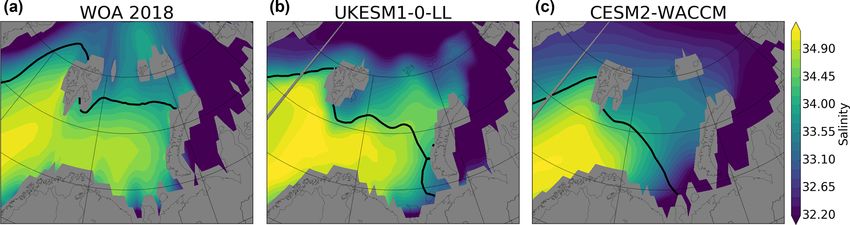
2222                                                   J. Terhaar et al.: Future Arctic Ocean acidification in CMIP6 models

quence the calcium carbonate (CaCO3 ) saturation states of         differences in brine rejection during sea ice formation, which
calcite and aragonite minerals (Haugan and Drange, 1996;           is critical to the formation of dense Arctic waters (Terhaar
Orr et al., 2005). The Arctic Ocean is particularly vulnera-       et al., 2019b).
ble to ocean acidification due to its naturally high dissolved
inorganic carbon concentrations, its low carbonate ion con-
                                                                   1.1   Emergent constraints on Arctic Ocean carbon
centrations, and its thus naturally low saturation states (Orr
                                                                         uptake and acidification
et al., 2005; Fabry et al., 2009; Gattuso and Hansson, 2011;
Riebesell et al., 2013; AMAP, 2018).
   In contrast to most of the global ocean, Arctic Ocean acid-     Emergent constraints are a suite of statistical techniques that
ification is caused not solely by increasing Cant concentra-       relate observable trends or sensitivities across multi-model
tions (Anderson et al., 2010; Ulfsbo et al., 2018; Terhaar         ensembles to differences in model projections in order to re-
et al., 2020a, b) but also by freshening (Koenigk et al., 2013;    duce future uncertainties (Allen and Ingram, 2002; Hall et al.,
Nummelin et al., 2016; Shu et al., 2018; Brown et al., 2020;       2019). An elegant early application that demonstrates many
Woosley and Millero, 2020). Fresh water from rivers, precip-       of the principles of emergent constraints is that of Hall and
itation, and sea ice typically has much lower total alkalinity     Qu (2006). In their study of models that contributed to the In-
(AT ) and total dissolved inorganic carbon (CT ) concentra-        tergovernmental Panel on Climate Change’s Fourth Assess-
tions than the ocean and therefore, in the absence of indi-        ment Report (AR4), Hall and Qu found a strong positive cor-
rect impacts on other fluxes, dilutes both marine AT and CT        relation between the magnitude of a model’s snow albedo
(Xue and Cai, 2020). As freshwater AT and CT concentra-            feedback on present-day seasonal timescales and under fu-
tions are generally similar, freshwater fluxes into the ocean      ture climate change. They concluded that relevant model bi-
typically act to reduce the difference between AT and CT ,         ases were consistent across these contrasting timescales and
decreasing marine CO2−  3 concentrations and ocean pH (Bates       therefore observations of the seasonal snow albedo feedback
et al., 2009; Bates and Mathis, 2009; Yamamoto-Kawai et al.,       could be used to constrain the ensemble range of the pro-
2011; Waldbusser and Salisbury, 2014; Wanninkhof et al.,           jected snow albedo feedback under climate change. Since
2015; Xue and Cai, 2020). In the Arctic Ocean, projected           the publication of Hall and Qu (2006), emergent constraint
freshening over the 21st century is larger than in most other      approaches have been applied extensively within the Earth
ocean regions due to ongoing sea ice melt, positive precipita-     sciences to constrain, amongst other things, projections of
tion minus evaporation, and large river runoff (Rawlins et al.,    climate sensitivity (Caldwell et al., 2018), Arctic sea ice ex-
2010; Rudels, 2015; Shu et al., 2018).                             tent (Boé et al., 2009), precipitation extremes (O’Gorman,
   Due to freshening and increasing Cant concentrations,           2012; DeAngelis et al., 2016), carbon cycle feedbacks (Cox
the Arctic Ocean is projected to be the first large-scale          et al., 2013; Wenzel et al., 2014), and marine primary pro-
ocean region to become undersaturated with respect to              duction (Kwiatkowski et al., 2017).
the metastable CaCO3 polymorph aragonite (arag < 1)                  Recently Terhaar et al. (2020a) showed that an emergent
(Steinacher et al., 2009). Under the Representative Concen-        constraint could be applied to CMIP5 projections of the Arc-
tration Pathway 8.5 (RCP8.5) high-emissions scenario, Arc-         tic Ocean Cant inventory and coincident acidification over
tic Ocean mesopelagic waters may even become undersatu-            the 21st century. As the Cant increase in the Arctic Ocean
rated with respect to the more stable CaCO3 polymorph cal-         is mainly driven by the inflow of Cant -rich waters from the
cite (calc < 1) before 2100 (Terhaar et al., 2020a). Arago-       Atlantic and their subsequent subduction in the Barents Sea
nite and calcite undersaturation is likely to affect the growth,   (Midttun, 1985; Rudels et al., 1994, 2000; Jeansson et al.,
reproduction, and survival of calcifying organisms, such as        2011; Smedsrud et al., 2013), the capability of each model
sea butterflies (Comeau et al., 2010) and foraminifera (Davis      to form dense surface waters in the Barents Sea was shown
et al., 2017), and could have ramifications for the wider          to strongly influence the future Arctic Ocean Cant inventory.
Arctic ecosystem (Armstrong et al., 2005; Karnovsky et al.,        By constraining simulated surface water densities with ob-
2008), including some of its most iconic predators, such as        servations, uncertainties related to the end-of-century Arctic
grey whales and walruses (Jay et al., 2011; AMAP, 2018).           Ocean Cant inventory in 2100 were reduced by around one-
   Projections of Arctic Ocean acidification over the 21st         third, and the best estimate under RCP8.5 was increased by
century had considerable subsurface uncertainties in the sim-      20 % to 9.0±1.6 Pg C (Terhaar et al., 2020a). Along with the
ulations conducted as part of the Coupled Model Intercom-          projected Cant inventory, uncertainties in the projected asso-
parison Project Phase 5 (CMIP5) (Steiner et al., 2013; Ter-        ciated basin-wide Arctic Ocean acidification could also be re-
haar et al., 2020a), with projected end-of-century basin-wide      duced in CMIP5. It should be noted, however, that in CMIP5
arag in mesopelagic waters ranging from 0.61 to 1.05. This        projected freshening and reductions in alkalinity were of mi-
large uncertainty has been attributed to multiple factors, in-     nor importance for Arctic Ocean acidification over the 21st
cluding variable inflow of Atlantic waters and their subse-        century. Moreover, the models have been shown to underes-
quent subduction; difficulties resolving the narrow passages       timate historical freshwater fluxes (1992–2012) in the Arc-
between the Arctic Ocean and its surrounding basins; and           tic Ocean by around 50 % (Shu et al., 2018), which suggests

Biogeosciences, 18, 2221–2240, 2021                                                  https://doi.org/10.5194/bg-18-2221-2021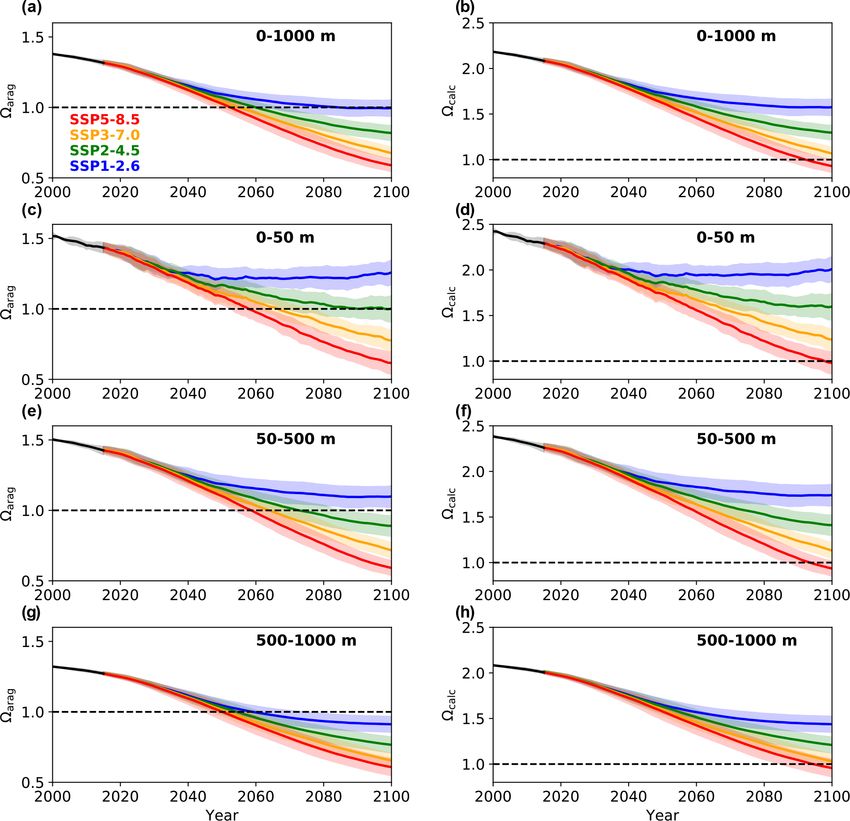
J. Terhaar et al.: Future Arctic Ocean acidification in CMIP6 models                                                       2223

they might also have underestimated freshwater fluxes over        2     Methods
the 21st century.
   Given that emergent constraints in many cases conflict         2.1    Arctic Ocean
with one another (Caldwell et al., 2018; Brient, 2020) and
can even be derived from data-mined pseudocorrelations            The Arctic Ocean was defined as the water north of the Fram
(Caldwell et al., 2014), it is critical to test published con-    Strait, the Barents Sea Opening, the Bering Strait, and the
straints, and the mechanisms that underpin them, across           Baffin Bay following Bates and Mathis (2009). This is con-
Earth system model (ESM) generations (Eyring et al., 2019;        sistent with the previously published emergent constraint on
Hall et al., 2019). The CMIP6 simulations provide such an         projected Arctic Ocean Cant and acidification (Terhaar et al.,
opportunity (Schlund et al., 2020).                               2020a).

1.2   From CMIP5 to CMIP6 models and simulations                  2.2    Earth system models
During the transition from CMIP5 to CMIP6, ESMs have              An ensemble of 14 ESMs from CMIP6 (Table 1) was used
generally improved the simulation of ocean dynamics and           with one ensemble member per model. All models follow
marine biogeochemistry (Séférian et al., 2020). Across most       the biogeochemical protocols outlined in Orr et al. (2017).
ESMs, the horizontal and/or vertical resolution of ocean          Riverine input of CT and AT is included in six ESMs (Ta-
models has increased, which potentially has large effects on      ble 1). The absence of CT and AT in riverine freshwater input
the representation of Arctic Ocean circulation, sea ice dy-       causes an overly strong reduction of CO2−   3 concentrations
namics (Docquier et al., 2019), and the carbon cycle (Terhaar     and thus low-biased saturation states in coastal regions but is
et al., 2019b). Ocean biogeochemical model components in          of minor importance on the pan-Arctic scale (Terhaar et al.,
CMIP6 also tend to have a more complex representation of          2019a). The spin-up length for each model varied between
the carbon and nutrient cycles than in CMIP5. In particular,      500 years (IPSL-CM6A-LR) and 12 000 years (MPI-ESM1-
the treatment of organic matter carbon cycling has generally      2-LR) (Séférian et al., 2020).
evolved, with remineralization of particles in sediments now         For each model, monthly 3D fields of dissolved inorganic
simulated in 10 out of 14 ESMs. These developments will           carbon, total alkalinity, dissolved inorganic phosphorus and
likely have a large effect on simulating the Arctic Ocean bio-    silicon, temperature, and salinity were used. All 3D fields
geochemistry given that 50 % of the Arctic Ocean is made          were regridded to the regular 1◦ × 1◦ grid with 33 depth lev-
up of shelf seas (Jakobsson, 2002), where sedimentation and       els used in the GLobal Ocean Data Analysis Project Version
sediment remineralization are crucial components of the car-      2 (GLODAPv2) observational product (Lauvset et al., 2016)
bon and nutrient cycle (Brüchert et al., 2018; Grotheer et al.,   to add simulated changes of these variables over the 21st cen-
2020). Furthermore, the external carbon and nutrient sources      tury to observations of the present-day mean state (see be-
from glaciers, atmospheric deposition, and rivers are repre-      low).
sented in more models in CMIP6 (Table 1) (Séférian et al.,           Cant was defined as the difference between annual means
2020). Riverine inputs in particular have been shown to be of     of dissolved inorganic carbon in the historical (1850–2014)
importance for present-day Arctic Ocean acidification (An-        simulations merged with the respective shared socioeco-
derson et al., 2010; Tank et al., 2012) and its future changes    nomic pathway (SSP1-2.6, SSP2-4.5, SSP3-7.0, and SSP5-
(Terhaar et al., 2019a).                                          8.5; 2015–2100; Riahi et al., 2017) and the concurrent pre-
   In this study, we extend recent CMIP6 ocean biogeochem-        industrial control simulations of each model. Output from 13
ical assessments (e.g. Séférian et al., 2020; Kwiatkowski         models was available for SSP1-2.6, output from 12 models
et al., 2020) and previous attempts to constrain projected        for SSP2-4.5 and SSP3-7.0, and output from 14 models for
Arctic Ocean Cant uptake by                                       SSP5-8.5 (Table 1).
 1. assessing projections of the Arctic Ocean Cant inventory         Changes in AT over the 21st century were calculated by
    over the 21st century in CMIP6 simulations                    subtracting changes in the pre-industrial control simulations
                                                                  from changes in the respective SSP. To quantify the effect
 2. exploring the role of Cant inventory increases and fresh-     of freshening on changes in AT , the AT anomalies for each
    ening in driving concurrent basin-wide ocean acidifica-       model were further decomposed into changes resulting from
    tion in the Arctic Basin                                      freshening and from the combined effect of other biogeo-
                                                                  chemical processes by calculating the temporal evolution of
 3. revaluating previous emergent constraints on the Arctic       salinity-corrected alkalinity with a reference salinity of 35
    Ocean Cant inventory and associated acidification us-         following Lovenduski et al. (2007). A zero-alkalinity end-
    ing the CMIP6 model ensemble and multiple future-             member was assumed for fresh water. This assumption is cor-
    emissions scenarios.                                          rect for models with no alkalinity in fresh water but an over-
                                                                  estimation for models with finite alkalinity concentrations in
                                                                  freshwater inputs (Table 1). Unfortunately, information on al-

https://doi.org/10.5194/bg-18-2221-2021                                                  Biogeosciences, 18, 2221–2240, 2021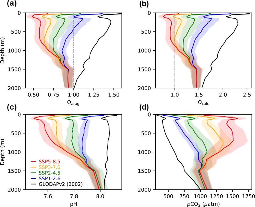
2224                                                          J. Terhaar et al.: Future Arctic Ocean acidification in CMIP6 models

Table 1. The CMIP6 ESMs used in this study with their ocean–sea ice and marine-biogeochemical (MBG) model components plus their
biogeochemical (BGC) riverine input.

    Model                                   Ocean–sea ice           MBG             Riverine BGC fluxes   Data DOI
    ACCESS-ESM1.5                           MOM5, CICE4             WOMBAT          None                  Ziehn et al. (2019a, b)
    (Ziehn et al., 2020)
    CanESM5                                 NEMO 3.4.1-LIM2         CMOC            None                  Swart et al. (2019a, b)
    (Swart et al., 2019e)
    CanESM5-CanOE                           NEMO 3.4.1-LIM2         CanOE           None                  Swart et al. (2019c, d)
    (Swart et al., 2019e;
    Christian et al., 2021)
    CESM2                                   POP2-CICE5              MARBL-BEC       C, N, P, Fe, Si, AT   Danabasoglu (2019a, b)
    (Danabasoglu et al., 2020)
    CESM2-WACCM                             POP2-CICE5              MARBL-BEC       C, N, P, Fe, Si, AT   Danabasoglu (2019c, d)
    (Danabasoglu et al., 2020)
    CNRM-ESM2-1                             NEMOv3.6-GELATOv6       PISCESv2-gas    C, P, AT              Seferian (2018a, b)
    (Séférian et al., 2019)
    GFDL-CM4a                               MOM6, SIS2              BLINGv2         C, N, P, Fe, AT       Guo et al. (2018a, b)
    (Held et al., 2019;
    Dunne et al., 2020a)
    GFDL-ESM4                               MOM6, SIS2              COBALTv2        C, P, N, AT           Krasting et al. (2018),
    (Dunne et al., 2020b;                                                                                 John et al. (2018)
    Stock et al., 2020)
    IPSL-CM6A-LR                            NEMOv3.6-LIM3           PISCESv2        C, N, P, Fe, Si, AT   Boucher et al. (2018a, b)
    (Boucher et al., 2020)
    MIROC-ES2L                              COCO                    OECO2           N, P                  Hajima et al. (2019),
    (Hajima et al., 2020)                                                                                 Tachiiri et al. (2019)
    MPI-ESM1.2-HR                           MPIOM                   HAMOCC6         None                  Schupfner et al. (2019),
    (Müller et al., 2018;                                                                                 Jungclaus et al. (2019)
    Mauritsen et al., 2019)
    MPI-ESM1.2-LR                           MPIOM                   HAMOCC6         None                  Wieners et al. (2019a, b)
    (Mauritsen et al., 2019)
    MRI-ESM2b                               MRICOM4                 NPZD            None                  Yukimoto et al. (2019b, c)
    (Yukimoto et al., 2019a)
    UKESM1-0-LL                             NEMO v3.6, CICE         MEDUSA-2        None                  Tang et al. (2019),
    (Sellar et al., 2019)                                                                                 Good et al. (2019)
   a Only SSP2-4.5 and SSP5-8.5. b Only SSP5-8.5.

kalinity concentrations in fresh water is not available for all           the year 2002, were used to calculate present-day arag and
models. Moreover, with the available model output, we can-                calc , pH, and pCO2 using the mocsy2.0 routine (Orr and
not quantify the individual contributions of land ice melt, sea           Epitalon, 2015) and the equilibrium constants recommended
ice melt, precipitation minus evaporation, and riverine input             for best practices (Dickson et al., 2007). Future arag and
to freshwater changes. Thus, for simplicity a zero-alkalinity             calc , pH, and pCO2 were calculated for each model as the
endmember was assumed for all models.                                     sum of the simulated changes in CT , AT , dissolved inorganic
   Ocean carbon chemistry variables in ESMs commonly                      phosphorus and silicon, temperature, and salinity from 2002
exhibit mean state biases (Orr et al., 2005; Steiner et al.,              onwards and the observed quantities in 2002.
2013). Therefore, observations of CT , AT , dissolved inor-                  The present-day maximum sea surface density in the Arc-
ganic phosphorus and silicon, temperature, and salinity from              tic Ocean was calculated from monthly climatologies over
GLODAPv2 (Lauvset et al., 2016), which is normalized to                   1986–2005, constructed from the respective salinity and tem-

Biogeosciences, 18, 2221–2240, 2021                                                         https://doi.org/10.5194/bg-18-2221-2021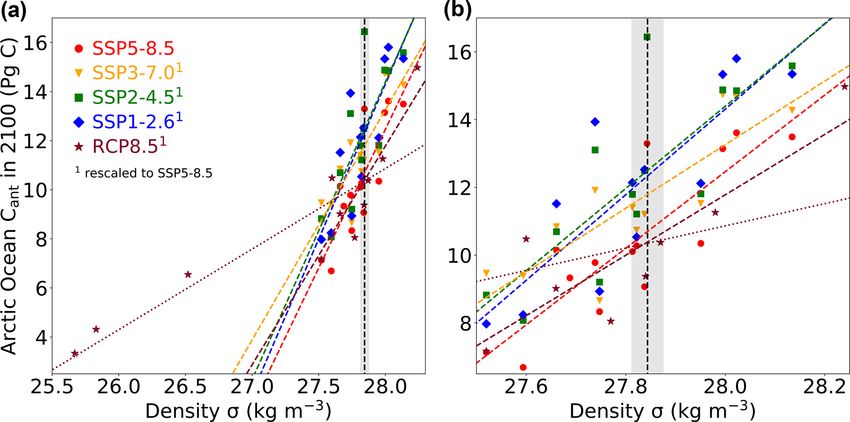
J. Terhaar et al.: Future Arctic Ocean acidification in CMIP6 models                                                     2225

perature outputs of each model. Maximum sea surface den-         the same radiative forcing, such as SSP5-8.5 and RCP8.5, it
sity was calculated, as in Terhaar et al. (2020a), as the mean   permits a first-order comparison.
density of the densest 5 % of Arctic surface waters (95th-
percentile waters) over all 12 months of the year.               2.5     Observational constraints

2.3   Simulations                                                As for the ESMs, the maximum sea surface density was cal-
                                                                 culated based on a monthly sea surface density climatol-
The simulations performed within CMIP5 were not forced           ogy on a regular 1◦ × 1◦ grid, which was constructed from
with the same atmospheric CO2 concentrations as the simu-        observed monthly salinity and temperature climatologies in
lations performed under CMIP6. In CMIP5, historically ob-        the World Ocean Atlas 2018 (Locarnini et al., 2018; Zweng
served atmospheric CO2 concentrations were used from 1850        et al., 2018).
to 2005 (Meinshausen et al., 2011). From 2006 onwards, the          The density uncertainty was calculated from the temper-
CO2 concentrations follow the different RCPs. In CMIP6,          ature and salinity uncertainties that were reported by the
the historical period was extended until 2014, and thereafter    World Ocean Atlas following standard propagation of un-
CO2 concentrations follow the different SSPs (Meinshausen        certainty. The total uncertainty is a combination of (1) the
et al., 2019).                                                   standard deviations for sea surface density derived from pub-
   The different land and energy use assumptions in the SSPs     lished standard deviations of sea surface temperature and
(Riahi et al., 2017) compared to the RCPs (O’Neill et al.,       salinity for each grid cell and each month in the World Ocean
2016) lead to higher atmospheric CO2 trajectories over the       Atlas 2018, and (2) the standard deviation from the weighted
21st century for the Tier 1 SSPs (Meinshausen et al., 2019)      mean of the 95th-percentile-density waters (Terhaar et al.,
compared to their RCP counterparts (Meinshausen et al.,          2020a).
2011), which results in globally greater surface ocean acidi-
fication in CMIP6 compared to CMIP5 (Kwiatkowski et al.,         2.6     Emergent constraints and probability density
2020). Historical atmospheric CO2 concentrations were also               functions of Cant
refined with additional data available since CMIP5 (Mein-
                                                                 To calculate the emergent constraint, first an ordinary least-
shausen et al., 2017). This refinement did not change the
                                                                 squares regression was calculated between the simulated
average atmospheric CO2 concentration from 1850 to 2005
                                                                 present-day maximum sea surface density and the Arctic
(1pCOatm 2 = 0 ± 1 ppm) but did change annual CO2 concen-        Ocean Cant inventory in 2100 for each ESM of the CMIP6
tration for single years by up to ±2 ppm. Furthermore, global
                                                                 model ensemble. The uncertainty range was estimated using
CO2 concentrations were additionally provided as monthly
                                                                 the 1σ prediction interval. In a second step the probability
latitudinally resolved concentrations, with model groups free
                                                                 density function (PDF) from the observations was convo-
to choose the forcing files they use (Meinshausen et al.,
                                                                 luted with the PDF from the linear regression, assuming a
2017, 2019).
                                                                 Gaussian distribution in both cases. The convolution of both
                                                                 PDFs is the constrained projection of the Arctic Ocean Cant
2.4   Cant scaling
                                                                 inventory following previous studies (Cox et al., 2013; Wen-
                                                                 zel et al., 2014; Kwiatkowski et al., 2017). The PDFs for un-
The different atmospheric CO2 trajectories over the 21st cen-
                                                                 constrained projections of the Cant inventory were calculated
tury between CMIP5 and CMIP6 complicates a comparison
                                                                 using equal weights for each model and assuming a Gaussian
of simulated Arctic Ocean Cant inventories between model
                                                                 distribution.
generations. To nevertheless compare the simulated Arctic
                                                                    Extending the analysis of Terhaar et al. (2020a), PDFs for
Ocean Cant , we used the commonly applied scaling approach
                                                                 the constrained projections of the Cant inventory were cal-
that assumes that the change in marine Cant is proportional
                                                                 culated not only for the year 2100 but for each year from
to the atmospheric Cant concentration (Gloor et al., 2003;
                                                                 2002 to 2100 and not only for the highest-emission scenario
Mikaloff Fletcher et al., 2006; Gerber et al., 2009; Gruber
                                                                 (RCP8.5) but for the four SSPs (SSP1-2.6, SSP2-4.5, SSP3-
et al., 2009). Under this assumption, the Cant inventory in
                                                                 7.0, and SSP5-8.5).
2100 for each scenario (RCP8.5, SSP1-2.6, SSP2-4.5, SSP3-
7.0) is linearly rescaled to that of SSP5-8.5 by multiplying
the simulated Arctic Ocean Cant inventory under the respec-      3     Results
tive scenario by the ratio of the mean atmospheric Cant con-
centration from 1850 to 2100 in SSP5-8.5 and the respective      3.1     Arctic Ocean Cant inventory
scenario.
   This approximation is likely imprecise when very different    3.1.1    Multi-model mean
scenarios are compared, such as SSP1-2.6 and SSP5-8.5, as
the effects of circulation changes, sea ice melt, and warming    Over the historical period from 1850 to 2005, the CMIP6
are not considered. However, when comparing scenarios with       ESMs simulate an Arctic Ocean Cant increase of 2.1 ± 0.6 Pg

https://doi.org/10.5194/bg-18-2221-2021                                                 Biogeosciences, 18, 2221–2240, 2021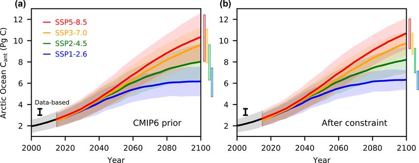
2226 J. Terhaar et al.: Future Arctic Ocean acidification in CMIP6 models
ated uncertainties (−29 % to −31 %) resulting in greater sep-
aration of the SSPs (Fig. 1).
3.2 Ocean acidification
3.2.1 Multi-model mean
Over the 21st century, ocean acidification leads to a reduction
in arag and calc (Fig. 3). Until around 2040, the reduction
Figure 1. Arctic Ocean Cant inventory over the 21st century. (a) of both saturation states averaged over the upper 1000 m is
Time series of multi-model mean Arctic Ocean Cant inventory over
independent of the SSP. From 2040 onwards, the rate of the
the 21st century for SSP1-2.6 (blue), SSP2-4.5 (green), SSP3-7.0
reduction depends on the pathway, and by 2100 basin-wide
(orange), and SSP5-8.5 (red) with the respective standard deviation
across the model ensemble (shading) (n = 12–14). The bars on the arag averaged over the upper 1000 m reaches 1.00 ± 0.06
right side of panels indicate the inter-model standard deviation in (SSP1-2.6), 0.82 ± 0.05 (SSP2-4.5), 0.66 ± 0.04 (SSP3-7.0),
the year 2100. (b) Time series of Arctic Ocean Cant inventory for and 0.59 ± 0.05 (SSP5-8.5), while calc reaches 1.56 ± 0.09
each scenario after the emergent constraint is applied. (SSP1-2.6), 1.29 ± 0.08 (SSP2-4.5), 1.06 ± 0.06 (SSP3-7.0),
and 0.92 ± 0.05 (SSP5-8.5).
The upper 1000 m of the Arctic Ocean is projected to be
C (inter-model standard deviation; Fig. 1a). Thus, the CMIP6 on average undersaturated with respect to aragonite by 2100
ESMs simulate an Arctic Ocean Cant inventory in 2005 that under all of the SSPs, with arag in SSP1-2.6 just below 1
is 36 % below the data-based estimate for the period from (0.995). Vertically, the entire water column will be undersat-
1765 to 2005 of 3.3 ± 0.3 Pg C (Terhaar et al., 2020b). urated with respect to aragonite in 2100 for all pathways but
Over the 21st century the Arctic Ocean Cant inventory in- SSP1-2.6 (Fig. 4). Under this low-emissions pathway, Arctic
creases depending on the SSP. Following the low-emission Ocean waters above 500 m are projected to remain supersat-
pathway SSP1-2.6 leads to a projected Arctic Ocean Cant urated with respect to aragonite, while those below 500 m
inventory in 2100 of 6.2 ± 1.3 Pg C. With increasing atmo- are projected to be undersaturated. For the more stable cal-
spheric Cant concentrations from SSP1-2.6 to SSP5-8.5, the cium carbonate polymorph calcite, basin-wide Arctic Ocean
projected Arctic Ocean Cant inventory in 2100 also increases, undersaturation is only projected under SSP5-8.5. Under this
resulting in 8.0 ± 1.7 for SSP2-4.5, 9.6 ± 1.6 for SSP3-7.0, high-emissions pathway, basin-wide undersaturation is pro-
and 10.3 ± 2.2 Pg C for SSP5-8.5. The relatively large un- jected for the water masses between 50 and 800 m.
certainties across the model ensemble (17–21 %) result in an Alongside declines in calcium carbonate saturation states,
overlap of the simulated Cant inventories in 2100 for SSP2- pH and pCO2 are also projected to change over the 21st
4.5, SSP3-7.0, and SSP5-8.5 within ±1 SD. century. Basin-wide averaged pH in the upper 1000 m de-
creases from 8.06 in 2002 to 7.88 ± 0.02 (SSP1-2.6), 7.79 ±
3.1.2 Constrained results 0.03 (SSP2-4.5), 7.68 ± 0.03 (SSP3-7.0), and 7.61 ± 0.03
(SSP5-8.5), while basin-wide averaged pCO2 in the upper
As was shown for RCP8.5 in the CMIP5 model ensemble 1000 m increases to 739 ± 38 (SSP1-2.6), 918 ± 75 (SSP2-
(Terhaar et al., 2020a), a linear relationship between maxi- 4.5), 1209±92 (SSP3-7.0), and 1428±124 µatm (SSP5-8.5).
mum sea surface density and the Arctic Ocean Cant inven- The lowest pH values and highest pCO2 values are projected
tory in 2100 is found across the CMIP6 model ensemble for to occur between 100 and 1000 m from the surface (Fig. 4).
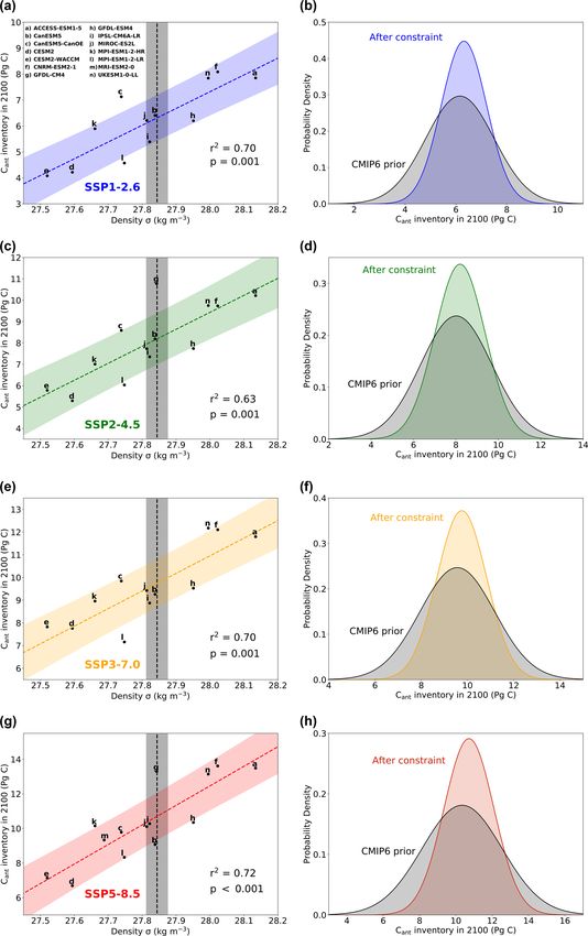
all four of the SSPs (r 2 = 0.63–0.72; Fig. 2a, c, e, and g).
By deriving a similar relationship for the projected Cant in- 3.2.2 Emergent constraints on acidification
ventory in all years from 2000 to 2100 and combining this
with observations of present-day sea surface density, the un- The emergent relationship between observed maximum sea
certainty of the projected Arctic Ocean Cant inventory can surface density and end-of-century Arctic Ocean acidifica-
be reduced throughout the 21st century (Fig. 1b). The emer- tion that was previously identified in CMIP5 models (Ter-
gent relationship is significant over all years from 2015 to haar et al., 2020a) does not exist anymore in the new CMIP6
2100 (p < 0.05) and the r 2 increases from 0.39 in 2014 to model generation (Fig. 5). Despite the emergent constraint
0.63–0.72 in 2100 depending on the scenario. In the year approach still functioning for projections of the Arctic Ocean
2100, this results in Arctic Ocean Cant inventory estimates of Cant inventory in CMIP6, this no longer translates into an
6.3 ± 0.9 (SSP1-2.6), 8.2 ± 1.2 (SSP2-4.5), 9.8 ± 1.1 (SSP3- emergent constraint for Arctic Ocean arag and calc . How-
7.0), and 10.7 ± 1.4 Pg C (SSP5-8.5) (Fig. 2b, d, f, and h). ever, if all changes in ocean biogeochemistry with the excep-
Thus, the emergent constraint is shown to slightly increase tion of alkalinity, which is kept constant at observed levels
the CMIP6 multi-model mean projected Cant inventory for from 2002 (Lauvset et al., 2016), are considered when esti-
each SSP (+2 % to +4 %) and substantially reduce associ- mating changes in arag and calc , emergent relationships
Biogeosciences, 18, 2221–2240, 2021 https://doi.org/10.5194/bg-18-2221-2021J. Terhaar et al.: Future Arctic Ocean acidification in CMIP6 models 2227 Figure 2. Emergent constraint on Arctic Ocean Cant inventory in 2100. Maximum Arctic Ocean sea surface density (95th percentile) and Arctic Ocean Cant inventory in 2100 for 12–14 ESMs for (a) SSP1-2.6 (blue), (c) SSP2-4.5 (green), (e) SSP3-7.0 (orange), and (g) SSP5- 8.5 (red). The ordinary least-squares regressions (dashed lines) and the ±1σ prediction intervals (shaded area) are shown for each SSP. Probability density functions before and after applying the emergent constraint for (b) SSP1-2.6, (d) SSP2-4.5, (f) SSP3-7.0, and (h) SSP5- 8.5. https://doi.org/10.5194/bg-18-2221-2021 Biogeosciences, 18, 2221–2240, 2021
2228                                                     J. Terhaar et al.: Future Arctic Ocean acidification in CMIP6 models

Figure 3. Basin-wide Arctic Ocean calcium carbonate saturation states over the 21st century. Time series of multi-model mean basin-wide
saturation states of aragonite from 2000 to 2014 (black) and from 2015 to 2100 for SSP1-2.6 (blue), SSP2-4.5 (green), SSP3-7.0 (orange),
and SSP5-8.5 (red) averaged (a) from 0 to 1000 m, (c) from 0 to 50 m, (e) from 50 to 500 m, and (g) from 500 to 1000 m with ±1 SD
(n = 12–14) shown as a shaded area. The differences when changing from historical simulations to the SSPs result from the different number
of ensemble members that are available for each simulation. (b, d, f, h) The same time series but for calcite.

are still found between maximum sea surface density and                inventory that was simulated by the previous model genera-
arag across all SSPs (r 2 = 0.54–0.73). When decreases in             tion (1.3 ± 0.7 Pg C) (Terhaar et al., 2020a).
alkalinity (AT ) are also taken into account, arag and calc             At the end of the 21st century, the unconstrained simulated
decrease further, and the emergent relationship disappears             Arctic Ocean Cant inventory under SSP5-8.5 is 37 % larger
(r 2 = 0.01–0.12).                                                     and the uncertainty is 19 % smaller than the unconstrained
                                                                       simulated Cant inventory in 2100 under RCP8.5 (7.5 ± 2.9 Pg
                                                                       C) (Terhaar et al., 2020a). After applying the constraint,
3.3    Comparison between CMIP5 and CMIP6                              the Arctic Ocean Cant inventory in 2100 under SSP5-8.5
                                                                       (10.7 ± 1.4 Pg C) is 19 % larger than the constrained Arc-
Compared to ESMs from CMIP5, the new generation of                     tic Ocean Cant inventory under RCP8.5 (9.0±1.6 Pg C). This
ESMs (CMIP6) has improved in simulating the maximum                    difference is of the same order of magnitude as the difference
Arctic Ocean sea surface density. Specifically, negative den-          in prescribed atmospheric CO2 concentration over the 21st
sity biases have been reduced, and the inter-model range               century, which is higher in SSP5-8.5 (CMIP6) than RCP8.5
in maximum sea surface density has substantially decreased             (CMIP5) (Meinshausen et al., 2011, 2019) and therefore re-
from 3.6 in CMIP5 (Terhaar et al., 2020a) to 0.9 kg m−3 in             sults in greater surface ocean acidification for approximately
CMIP6 (Fig. 2). As a result, the inter-model range of the              the same radiative forcing (Kwiatkowski et al., 2020).
Cant inventory in the CMIP6 model ensemble is also re-                    To compare the emergent constraint across scenarios with
duced (Fig. 2). Moreover, without the negative maximum-                different atmospheric CO2 concentrations, the simulated
sea-surface-density bias, the simulated multi-model mean               Arctic Ocean Cant inventory in 2100 for each scenario was
Arctic Ocean Cant inventory in 2005 is 61 % higher than the            rescaled to SSP5-8.5 using the mean atmospheric Cant con-

Biogeosciences, 18, 2221–2240, 2021                                                        https://doi.org/10.5194/bg-18-2221-2021
J. Terhaar et al.: Future Arctic Ocean acidification in CMIP6 models 2229
Figure 6. Arctic Ocean Cant inventory in 2100, rescaled to SSP5-
8.5 atmospheric Cant concentrations (see Methods), against maxi-
mum Arctic Ocean sea surface density (95th percentile) for SSP1-
2.6 (blue diamonds; r 2 = 0.70), SSP2-4.5 (green squares; r 2 =
0.63), SSP3-7.0 (orange triangles; r 2 = 0.70), SSP5-8.5 (red cir-
cles; r 2 = 0.72), and RCP8.5 (purple stars; r 2 = 0.74) (a) over the
entire density range and (b) over the density range from 27.5 to
Figure 4. Vertical profile of basin-wide Arctic Ocean calcium car- 28.3 kg m−3 . The simulated Arctic Ocean Cant inventory in 2100
bonate saturation states, pH, and pCO2 in 2100. Multi-model mean for each scenario (Fig. 2) was rescaled to SSP5-8.5 using the mean
vertical profiles of (a) aragonite and (b) calcite saturation states, atmospheric Cant concentration from 1850 to 2100 as a scaling fac-
(c) pH, and (d) pCO2 in 2100 for SSP1-2.6 (blue), SSP2-4.5 tor. Linear fits use all available models for each scenario (coloured
(green), SSP3-7.0 (orange), and SSP5-8.5 (red) averaged (a) with dashed lines). For RCP8.5 an additional fit is shown excluding the
±1 SD (n = 12–14) shown as a shaded area. Observed profiles in three models with density anomalies below 27.5 kg m−3 (b) (dotted
2002 from GLODAPv2 are shown in black (Lauvset et al., 2016). purple line; r 2 = 0.79).
ever, the slope in CMIP5 increases to 8.9 Pg C kg−1 m3 if
the three CMIP5 models with particularly low maximum
sea surface densities (< 27.5 kg m−3 ) are excluded (dotted
line in Fig. 6). The resulting constrained estimate for the
rescaled Arctic Ocean Cant inventory decreases from the
low-emission scenario to the high-emission scenario from
12.3 to 10.7 Pg C. When comparing the two high-emission
scenarios, the rescaled Arctic Ocean Cant inventories are
10.7 (SSP5-8.5) and 10.4 Pg C (RCP8.5). The latter re-
mains unchanged if the three CMIP5 models with particu-
larly low maximum sea surface densities (< 27.5 kg m−3 ) are
excluded.
4 Discussion
4.1 Arctic Ocean Cant inventory
Figure 5. The CMIP6 ensemble relationship between end-of-
century arag and the Cant inventory in the Arctic Ocean. Basin-
Across the CMIP6 model ensemble, the Arctic Ocean Cant
wide arag averaged over the upper 1000 m with (orange) and with- storage over the 21st century is highly related to maximum
out (blue) taking into account concurrent changes in alkalinity (AT ) sea surface densities (Fig. 2), which predominately occur in
against the Arctic Ocean Cant inventory in the year 2100 for (a) the Barents Sea (Midttun, 1985; Smedsrud et al., 2013; Ter-
SSP1-2.6, (a) SSP2-4.5, (c) SSP3-7.0, and (d) SSP5-8.5. haar et al., 2020a). The inter-model range in maximum sea
surface density in the Barents Sea is mainly explained by dif-
ferences in sea surface salinities (r 2 = 0.93), which are influ-
centration from 1850 to 2100 as a linear scaling factor enced by brine rejection (Midttun, 1985; Årthun et al., 2011)
(Fig. 6). The relationship remains robust (r 2 = 0.63–0.74) and the strength of inflowing, saltier Atlantic waters through
for all five analysed scenarios. The slope of the emergent re- the Barents Sea Opening (Fig. 7). Compared to CMIP5 mod-
lationship is however substantially steeper in CMIP6 (9.4– els, the reduced negative bias of simulated maximum sea sur-
12.6 Pg C kg−1 m3 ) than in CMIP5 (3.3 Pg C kg−1 m3 ). How- face densities (Fig. 6) indicates model improvement in sim-
https://doi.org/10.5194/bg-18-2221-2021 Biogeosciences, 18, 2221–2240, 20212230 J. Terhaar et al.: Future Arctic Ocean acidification in CMIP6 models
start in 1850, data-based estimates account for all Cant since
1765. This leads to an underestimation of the global ocean
Cant inventory by ESMs of around 30 % (Bronselaer et al.,
2017) and of around 20 % in the Arctic Ocean (Terhaar et al.,
2019b). Even if we increased the constrained Arctic Ocean
Cant inventory in 2005 by 20 %, an underestimation of around
Figure 7. Annual mean sea surface salinity in the Barents Sea and 16 % would remain compared to the data-based estimate.
its neighbouring waters from (a) the World Ocean Atlas 2018 and This underestimation of the data-based estimate suggests that
from the CMIP6 model with the (b) highest (UKESM1-0-LL) and all ESMs are missing additional pathways of Cant entry into
(c) lowest (CESM2-WACCM) maximum sea surface density and the Arctic Ocean, other than the principal pathway via the
salinity. The 0 ◦ C isotherm indicates approximately the extent of Barents Sea. Indeed, small-scale density flows along conti-
Atlantic waters (black solid line). nental slopes can be observed in different regions of the Arc-
tic Ocean (Rudels et al., 1994; Jones et al., 1995) but cannot
be simulated by the coarse resolution of most ESMs. Thus,
ulating the circulation of Atlantic and Arctic surface waters. the constrained estimates of the Arctic Ocean Cant inventory
Despite the reduced inter-model range, the robust relation- presented here are likely still a lower boundary.
ship between maximum sea surface density and Cant across Recent observation of dilution of AT and CT in surface wa-
model generations (Fig. 6) supports evidence that inflowing ters of the Amerasian Basin caused by freshening have led
Atlantic waters through the Barents Sea Opening and their to the hypothesis that continuous freshening might turn the
transformation into deep and intermediate waters via brine Arctic Ocean from a sink of Cant into a source over the 21st
rejection are the dominant process governing Arctic Ocean century (Woosley and Millero, 2020). However, observations
Cant increases (Midttun, 1985; Rudels et al., 1994, 2000; in the Eurasian basins, which receive more saline Atlantic
Jeansson et al., 2011; Smedsrud et al., 2013). The application water and less freshwater input, still show increases of Cant
of observational constraints to this emergent multi-model re- concentrations (Ulfsbo et al., 2018) over a depth of 1500 m in
lationship in order to constrain the projected Arctic Ocean the last 20 years. The CMIP5 and CMIP6 model ensembles
Cant inventory (Fig. 2) and focus efforts on model develop- both simulate continuous accumulation of Cant in the Arctic
ment therefore remains promising. Ocean under all SSPs (Fig. 1), suggesting that the subduction
However, the slope of the linear relationship between of Cant -rich Atlantic waters in the Barents Sea remains larger
maximum sea surface density and the Arctic Ocean Cant than any loss of Cant in surface waters over the 21st cen-
inventory over the 21st century in the CMIP5 model en- tury. Nevertheless, the reduction of the storage rate of Cant
semble (3.3 ± 0.6 Pg C kg−1 m3 , scaled to SSP5-8.5 atmo- under SSP5-8.5 (Fig. 1) in combination with constantly in-
spheric Cant concentrations) is 3–4 times less than that creasing atmospheric CO2 concentrations (Riahi et al., 2017)
in the CMIP6 model ensemble (12.6 ± 2.6 for SSP1-2.6, indicates that dilution may reduce the capacity of the Arc-
12.1 ± 2.8 for SSP2-4.5, 9.4 ± 1.9 for SSP3-7.0, and 11.3 ± tic Ocean to store further Cant as suggested by Woosley and
2.0 Pg C kg−1 m3 for SSP5-8.5) (Fig. 6). The reduced slope Millero (2020).
in the CMIP5 ensemble is mainly caused by three mod-
els with maximum surface density anomalies well be- 4.2 Arctic Ocean acidification
low 27.5 kg m−3 . When these three models are excluded,
the remaining CMIP5 models follow a slope of 8.9 ± 4.2.1 arag and calc , pH, and pCO2 in 2100
2.2 Pg C kg−1 m3 , in broad agreement with the CMIP6 model
ensemble (Fig. 6). This suggests that the linear emergent re- Even under the most optimistic scenario assessed (SSP1-
lationship does not hold below a certain value of maximum 2.6), the Arctic Ocean will become on average undersatu-
sea surface density below which the impact on deep-water rated with respect to aragonite, with possible consequences
formation and subsequent Cant storage in the Arctic Ocean for calcifying organisms (Comeau et al., 2010) and the food
is limited. However, as the two linear relationships happen to chain (Armstrong et al., 2005; Karnovsky et al., 2008). In
cross the observed maximum sea surface density at nearly the this scenario only water masses above 500 m remain super-
same location (Fig. 6), the constrained Cant inventory for the saturated this century. These findings are in good agreement
CMIP5 model ensemble remains almost entirely unchanged with idealized estimates of arag and calc that project the
when the three low-density models are excluded. future Cant inventory based on the transient time distribu-
Even without the low-density bias in the Barents Sea, the tion method and observed CFC-12 concentrations (Anderson
constrained Arctic Ocean Cant inventory in 2005 in CMIP6 et al., 2010; Terhaar et al., 2020b).
remains 36 % below the data-based estimate (Terhaar et al., In addition to widespread Arctic Ocean undersaturation
2020b). This underestimation is partly due to the different with respect to aragonite, water masses between 50 and
definition of Cant in data-based estimates and ESMs. While 800 m are even projected to become undersaturated with
the historical simulations in CMIP5 and CMIP6 typically respect to calcite by the end of the century under SSP5-
Biogeosciences, 18, 2221–2240, 2021 https://doi.org/10.5194/bg-18-2221-2021J. Terhaar et al.: Future Arctic Ocean acidification in CMIP6 models 2231 8.5. Calcite undersaturation in Arctic Ocean subsurface wa- ters will likely further enhance the pressure on the Arc- tic Ocean ecosystem as calcite-forming organisms, such as foraminifera (Davis et al., 2017) and coccolithophores (Kottmeier et al., 2016), experience potential impacts on growth and survival. Furthermore, the projected increases in pCO2 (Fig. 4c and d) alongside projected increases in its seasonal amplitude (McNeil and Sasse, 2016; Kwiatkowski and Orr, 2018) are likely to lead to hypercapnic conditions that might directly affect the growth and survival of Arctic fish (Frommel et al., 2012; Schmidt et al., 2017; Kunz et al., 2018) under high- emissions scenarios. 4.2.2 Driving processes of acidification The CMIP6 model ensemble shows astonishingly good agreement with respect to projections of Arctic Ocean acidi- Figure 8. CMIP6 basin-wide changes in alkalinity (AT ) averaged fication over the 21st century. Compared to the CMIP5 model over the upper 1000 m from 2002 to 2100 caused by freshwater dilu- ensemble, the uncertainties in projected arag averaged over tion (blue) and changes in biogeochemistry (green) against the Arc- the upper 1000 m in 2100 have been reduced from 0.13 to tic Ocean Cant inventory for (a) SSP1-2.6, (b) SSP2-4.5, (c) SSP3- 0.04–0.06, and those for calc from 0.21 to 0.05–0.09. 7.0, and (d) SSP5-8.5. AT anomalies were decomposed by calculat- The main reason for the reduced uncertainty appears to be ing the temporal evolution of salinity-corrected alkalinity following that the ESMs that have a lower maximum sea surface den- Lovenduski et al. (2007). sity and that thus take up less Cant in the Arctic Ocean over the 21st century (Fig. 2) are the same models that simulate a stronger reduction in AT (Fig. 8). To explain this nega- changes in AT in CMIP5 compared to CMIP6 might have tive correlation between Cant uptake and reductions in AT , been caused by an underestimation of Arctic Ocean freshen- we propose the following mechanism: over the 21st century, ing over the 21st century given that the CMIP5 models also melting of sea ice, land ice, and increased river runoff are underestimated historical Arctic Ocean freshening by around projected to freshen the Arctic Ocean (Koenigk et al., 2013; 50 % in the Arctic Ocean (Shu et al., 2018). In the CMIP6 Nummelin et al., 2016; Shu et al., 2018) and to reduce AT model ensemble this negative bias with respect to freshwater (Fig. 8) (Woosley and Millero, 2020). In the CMIP6 ensem- fluxes and subsequent dilution of AT appears to have been ble, this freshening and reduction of AT tends to be stronger reduced. This is probably a consequence of better represen- in models with lower sea surface salinities and densities; i.e. tation of riverine fluxes as well as increased model resolution the models that simulate less inflow of saline Atlantic wa- and hence improved circulation (Séférian et al., 2020). ters, such as CESM2-WACCM (Fig. 7), have lower Barents To estimate the likely impacts of CT increases and AT de- Sea surface salinity and density, weak deep-water formation, creases to Arctic Ocean acidification over the 21st century, and therefore less Cant storage (Fig. 2). In contrast, models one can assess their relative contributions to acidification in with a larger inflow of saline Atlantic water have stronger constrained estimates of end-of-century Cant (dotted line in deep-water formation, greater Cant storage, less freshening, Fig. 5). In SSP5-8.5 for example, increasing CT along with and a smaller reduction in AT . This compensation then re- changes in temperature and salinity reduce arag from 1.38 to sults in a similar simulated reduction of arag and calc over 0.75, while decreasing AT further reduces this to 0.59. Thus, the 21st century across all models in the CMIP6 ensemble, the future storage of Cant in the Arctic Ocean still remains the through either a reduction in AT or an increase in CT . Other main driver of Arctic Ocean acidification, with acidification possible drivers, such as changes in temperature and salinity, further enhanced by decreases in AT . are likely of minor importance given the relatively good cor- relation between the projected Cant inventory and basin-wide reduction of arag and calc over the 21st century when AT 5 Conclusions is not taken into account (r 2 = 0.54–0.73). In the CMIP5 model ensemble, this compensation effect Earth system models tend to have improved their perfor- did not exist, and projected saturation states and pH were mance in the Arctic Ocean from CMIP5 to CMIP6. The neg- mainly driven by the projected Cant storage in each model ative bias with respect to present-day maximum sea surface (Terhaar et al., 2020a), with changes in AT , temperature, density is substantially reduced in CMIP6, and the historical and salinity being of minor importance. The relatively small Cant inventory is closer to the data-based estimate (Terhaar https://doi.org/10.5194/bg-18-2221-2021 Biogeosciences, 18, 2221–2240, 2021
2232                                                   J. Terhaar et al.: Future Arctic Ocean acidification in CMIP6 models

et al., 2020b). Furthermore, the inter-model range of pro-         there is clearly no need for such constraints when models are
jected arag and calc and the Cant inventory have been re-        in broad agreement.
duced. Uncertainties in the future Cant inventory under four          Independent of the driving mechanism, the projected Arc-
shared socioeconomic pathways can be further reduced by            tic Ocean acidification over the 21st century has possibly
applying the previously identified emergent constraint be-         grave consequences for the wider Arctic Ocean ecosystem
tween present-day maximum Arctic Ocean sea surface den-            (Gattuso and Hansson, 2011; Riebesell et al., 2013; AMAP,
sity and the future Cant inventory (Terhaar et al., 2020a).        2018). Under all socioeconomic pathways, the upper 1000 m
   Hall et al. (2019) define “confirmed” emergent constraints      of the Arctic Ocean will be on average undersaturated with
as fulfilling the following criteria: (1) a plausible mechanism,   respect to aragonite. Thus, keystone species like the sea
(2) verification of that mechanism, and (3) out-of-sample          butterfly (aragonitic pteropod Limacina helicina) may lose
testing. The mechanism underpinning the relationship be-           most to all of their suitable habitat in the Arctic Ocean
tween maximum sea surface densities and the projected Cant         (Comeau et al., 2010). However, under the low-emissions
inventory in the Arctic Ocean is consistent with observations      pathway SSP1-2.6 aragonite undersaturation is projected to
and has been verified in an ocean-only model at different          be avoided in the upper 500 m of the water column, pro-
resolutions (Terhaar et al., 2020a). The testing of this emer-     viding a potential refuge. Under the high-emissions path-
gent constraint in the CMIP6 ensemble can be considered out        way SSP5-8.5, water masses between 50 and 800 m are addi-
of sampling, although the extent of model independence be-         tionally projected to become undersaturated with respect to
tween generations remains questionable (Knutti et al., 2013;       calcite. While isolated regions of the surface Arctic Ocean
Sanderson et al., 2015). Despite the overall emergent con-         that are strongly influenced by riverine inputs are already
straint on projected Arctic Ocean Cant being similar between       seasonally undersaturated with respect to calcite (Bates and
CMIP6 and CMIP5, the change in the multi-model emer-               Mathis, 2009), subsurface Arctic waters would be the first to
gent relationship indicates that further validation is required.   exhibit annually averaged and basin-wide calcite undersatu-
Specifically, it appears that the linear relationship between      ration over a depth of several hundred metres. Vertically mi-
maximum sea surface densities and the projected Cant inven-        grating organisms that form calcite shells and skeletons, such
tory breaks down in models with extremely low-biased sea           as coccolithophores (Kottmeier et al., 2016) and foraminifera
surface densities, highlighting a potential limitation to this     (Davis et al., 2017), may lose their natural refugia to which
emergent constraint that requires further assessment.              they migrate during the day (Berge et al., 2015). These hos-
   While the mechanisms underlying emergent constraints on         tile conditions for calcifying organisms will likely cause their
the future Arctic Ocean Cant inventory appear to be consistent     decline, with unknown consequences for the wider Arctic
between CMIP5 and CMIP6, this is not the case for the pre-         food web (Armstrong et al., 2005; Karnovsky et al., 2008)
viously identified emergent constraint on ocean acidification      and its iconic species (Jay et al., 2011; AMAP, 2018).
variables (arag and calc , pH, and pCO2 ). In the CMIP6
model ensemble, projected model uncertainties in arag and
calc , pH, and pCO2 are dramatically reduced compared to          Data availability. The Earth system model output used in this study
the uncertainties in CMIP5 and are driven not only by the          is available via the Earth System Grid Federation (https://esgf-node.
increase in Cant but also by a reduction in AT due to pan-         ipsl.upmc.fr/projects/esgf-ipsl/, last access: 31 March 2021). For
Arctic freshening. A weak inflow of saline Atlantic waters in      further information, please see Table 1. Observations from the
                                                                   World Ocean Atlas 2018 (https://www.nodc.noaa.gov/OC5/woa18/,
ESMs results not only in lighter surface waters and less Cant
                                                                   last access: 3 January 2020; Locarnini et al., 2018; Zweng et al.,
storage over the 21st century but also in a stronger reduc-
                                                                   2018) and GLODAPv2 (https://www.nodc.noaa.gov/ocads/oceans/
tion of alkalinity caused by a stronger freshening. A strong       GLODAPv2_2019/, Lauvset et al., 2016) are available via the Na-
Atlantic inflow, however, appears to limit freshening and re-      tional Oceanic and Atmospheric Administration.
ductions in alkalinity but results in greater Cant storage. Al-
though both Cant storage and alkalinity reductions contribute
considerably to Arctic Ocean acidification, our results sug-       Author contributions. The study was led by JT, who made the fig-
gest that Cant remains the dominant process. In the CMIP5          ures and wrote the initial manuscript. TB and LK provided help
model ensemble, the influence of freshening on emergent            for the analyses and interpretation of the results. OT processed the
constraints on acidification variables might have been of lim-     CMIP6 model data (download, regridding). All authors contributed
ited importance because (a) freshening was largely underesti-      to the final manuscript.
mated (Shu et al., 2018) and (b) differences in simulating the
inflow of Atlantic waters through the Barents Sea Opening
were considerably larger across the model ensemble (Terhaar        Competing interests. The authors declare that they have no conflict
et al., 2020a). Thus, the absence of an emergent constraint        of interest.
on projected Arctic acidification in CMIP6 could be viewed
as a consequence of successful model development. Indeed,

Biogeosciences, 18, 2221–2240, 2021                                                    https://doi.org/10.5194/bg-18-2221-2021
J. Terhaar et al.: Future Arctic Ocean acidification in CMIP6 models 2233
Disclaimer. The work reflects only the authors’ view; the European O. J., Daase, M., and Falk-Petersen, S.: In the dark: A re-
Commission and their executive agency are not responsible for any view of ecosystem processes during the Arctic polar night,
use that may be made of the information the work contains. overarching perspectives of contemporary and future ecosys-
tems in the Arctic Ocean, Prog. Oceanog., 139, 258–271,
https://doi.org/10.1016/j.pocean.2015.08.005, 2015.
Acknowledgements. We acknowledge the World Climate Research Boé, J., Hall, A., and Qu, X.: September sea-ice cover in the Arctic
Programme’s Working Group on Coupled Modelling, which is re- Ocean projected to vanish by 2100, Nat. Geosci., 2, 341–343,
sponsible for CMIP. For CMIP the US Department of Energy’s Pro- https://doi.org/10.1038/ngeo467, 2009.
gram for Climate Model Diagnosis and Intercomparison provided Boucher, O., Denvil, S., Caubel, A., and Foujols, M. A.: IPSL
coordinating support and led the development of software infras- IPSL-CM6A-LR model output prepared for CMIP6 CMIP,
tructure in partnership with the Global Organization for Earth Sys- Tech. Rep., Version 20180803, Earth System Grid Federation,
tem Science Portals. We also thank the IPSL modelling group for https://doi.org/10.22033/ESGF/CMIP6.1534, 2018a.
the software infrastructure, which facilitated CMIP6 analysis. Boucher, O., Denvil, S., Caubel, A., and Foujols, M. A.: IPSL
IPSL-CM6A-LR model output prepared for CMIP6 Scenari-
oMIP, Tech. Rep., Version20190119, Earth System Grid Federa-
Financial support. This research has been supported by the Hori- tion, https://doi.org/10.22033/ESGF/CMIP6.1532, 2018b.
zon 2020 (4C (grant no. 821003), CRESCENDO (grant no. Boucher, O., Servonnat, J., Albright, A. L., Aumont, O., Balkan-
641816), and COMFORT (grant no. 820989)), the Schweizerischer ski, Y., Bastrikov, V., Bekki, S., Bonnet, R., Bony, S., Bopp, L.,
Nationalfonds zur Förderung der Wissenschaftlichen Forschung Braconnot, P., Brockmann, P., Cadule, P., Caubel, A., Cheruy,
(grant no. PP00P2_170687), the Agence Nationale de la Recherche F., Codron, F., Cozic, A., Cugnet, D., D’Andrea, F., Davini,
(grant no. ANR-18-ERC2-0001-01), and the Norges Forskningsråd P., de Lavergne, C., Denvil, S., Deshayes, J., Devilliers, M.,
(grant no. 275268). Ducharne, A., Dufresne, J.-L., Dupont, E., Éthé, C., Fairhead, L.,
Falletti, L., Flavoni, S., Foujols, M.-A., Gardoll, S., Gastineau,
G., Ghattas, J., Grandpeix, J.-Y., Guenet, B., Guez, Lionel,
E., Guilyardi, E., Guimberteau, M., Hauglustaine, D., Hour-
Review statement. This paper was edited by Jean-Pierre Gattuso
din, F., Idelkadi, A., Joussaume, S., Kageyama, M., Khodri,
and reviewed by Scott C. Doney and Claudine Hauri.
M., Krinner, G., Lebas, N., Levavasseur, G., Lévy, C., Li, L.,
Lott, F., Lurton, T., Luyssaert, S., Madec, G., Madeleine, J.-
B., Maignan, F., Marchand, M., Marti, O., Mellul, L., Meur-
References desoif, Y., Mignot, J., Musat, I., Ottlé, C., Peylin, P., Planton,
Y., Polcher, J., Rio, C., Rochetin, N., Rousset, C., Sepulchre, P.,
Allen, M. R. and Ingram, W. J.: Constraints on future changes Sima, A., Swingedouw, D., Thiéblemont, R., Traore, A. K., Van-
in climate and the hydrologic cycle, Nature, 419, 228–232, coppenolle, M., Vial, J., Vialard, J., Viovy, N., and Vuichard,
https://doi.org/10.1038/nature01092, 2002. N.: Presentation and Evaluation of the IPSL-CM6A-LR Cli-
AMAP: AMAP Assessment 2018: Arctic Ocean Acidification, mate Model, J. Adv. Model. Earth Sy., 12, e2019MS002 010,
Tech. Rep., Arctic Monitoring and Assessment Programme https://doi.org/10.1029/2019MS002010, 2020.
(AMAP), Tromsø, Norway, 2018. Brient, F.: Reducing uncertainties in climate projections with
Anderson, L., Tanhua, T., Björk, G., Hjalmarsson, S., Jones, emergent constraints: Concepts, Examples and Prospects, Adv.
E., Jutterström, S., Rudels, B., Swift, J., and Wåhlstöm, Atmos. Sci., 37, 1–15, https://doi.org/10.1002/2016GL069465,
I.: Arctic ocean shelf–basin interaction: An active continen- 2020.
tal shelf CO2 pump and its impact on the degree of cal- Bronselaer, B., Winton, M., Russell, J., Sabine, C. L., and Khati-
cium carbonate solubility, Deep-Sea Res. Pt. I, 57, 869–879, wala, S.: Agreement of CMIP5 simulated and observed ocean an-
https://doi.org/10.1016/j.dsr.2010.03.012, 2010. thropogenic CO2 uptake, Geophys. Res. Lett., 44, 12298–12305,
Armstrong, J. L., Boldt, J. L., Cross, A. D., Moss, J. H., Davis, https://doi.org/10.1002/2017GL074435, 2017.
N. D., Myers, K. W., Walker, R. V., Beauchamp, D. A., and Hal- Brown, K. A., Holding, J. M., and Carmack, E. C.: Understanding
dorson, L. J.: Distribution, size, and interannual, seasonal and Regional and Seasonal Variability Is Key to Gaining a Pan-Arctic
diel food habits of northern Gulf of Alaska juvenile pink salmon, Perspective on Arctic Ocean Freshening, Front. Mar. Sci., 7, 606,
Oncorhynchus gorbuscha, Deep-Sea Res. Pt. II, 52, 247–265, https://doi.org/10.3389/fmars.2020.00606, 2020.
https://doi.org/10.1016/j.dsr2.2004.09.019, 2005. Brüchert, V., Bröder, L., Sawicka, J. E., Tesi, T., Joye, S. P., Sun, X.,
Bates, N. R. and Mathis, J. T.: The Arctic Ocean marine carbon Semiletov, I. P., and Samarkin, V. A.: Carbon mineralization in
cycle: evaluation of air-sea CO2 exchanges, ocean acidification Laptev and East Siberian sea shelf and slope sediment, Biogeo-
impacts and potential feedbacks, Biogeosciences, 6, 2433–2459, sciences, 15, 471–490, https://doi.org/10.5194/bg-15-471-2018,
https://doi.org/10.5194/bg-6-2433-2009, 2009. 2018.
Bates, N. R., Mathis, J. T., and Cooper, L. W.: Ocean acidification Caldwell, P. M., Bretherton, C. S., Zelinka, M. D., Klein,
and biologically induced seasonality of carbonate mineral satu- S. A., Santer, B. D., and Sanderson, B. M.: Statisti-
ration states in the western Arctic Ocean, J. Geophys. Res., 114, cal significance of climate sensitivity predictors obtained
C11007, https://doi.org/10.1029/2008JC004862, 2009. by data mining, Geophys. Res. Lett., 41, 1803–1808,
Berge, J., Renaud, P. E., Darnis, G., Cottier, F., Last, K., Gabrielsen, https://doi.org/10.1002/2014GL059205, 2014.
T. M., Johnsen, G., Seuthe, L., Weslawski, J. M., Leu, E.,
Moline, M., Nahrgang, J., Søreide, J. E., Varpe, Ø., Lønne,
https://doi.org/10.5194/bg-18-2221-2021 Biogeosciences, 18, 2221–2240, 2021You can also read