Characterization of the air-sea exchange mechanisms during a Mediterranean heavy precipitation event using realistic sea state modelling ...
←
→
Page content transcription
If your browser does not render page correctly, please read the page content below
Atmos. Chem. Phys., 20, 1675–1699, 2020
https://doi.org/10.5194/acp-20-1675-2020
© Author(s) 2020. This work is distributed under
the Creative Commons Attribution 4.0 License.

Characterization of the air–sea exchange mechanisms
during a Mediterranean heavy precipitation event using
realistic sea state modelling
César Sauvage1 , Cindy Lebeaupin Brossier1 , Marie-Noëlle Bouin1,2 , and Véronique Ducrocq1
1 CNRM,Université de Toulouse, Météo-France/CNRS, Toulouse, France
2 CNRS,
      Ifremer, IRD, UBO/Laboratoire d’Océanographie Physique et Spatiale (LOPS),
UMR 6523, IUEM, Plouzané, France

Correspondence: César Sauvage (cesar.sauvage@meteo.fr)

Received: 27 August 2019 – Discussion started: 2 September 2019
Revised: 10 December 2019 – Accepted: 3 January 2020 – Published: 11 February 2020

Abstract. This study investigates the mechanisms acting at         1   Introduction
the air–sea interface during a heavy precipitation event that
occurred between 12 and 14 October 2016 over the north-            The western Mediterranean region is regularly affected by
western Mediterranean area and led to large amounts of rain-       heavy precipitation events (HPEs) that are characterized by a
fall (up to 300 mm in 24 h) over the Hérault region (southern      large amount of rainfall over a small area in a very short time;
France). The study case was characterized by a very strong         these events can lead to flash flooding, causing severe dam-
( > 20 m s−1 ) easterly to south-easterly wind at low level that   age and, in some cases, casualties (e.g. Delrieu et al., 2005;
generated very rough seas (significant wave height of up to        Llasat et al., 2013). Usually such events are generated by
6 m) along the French Riviera and the Gulf of Lion. In order       quasi-stationary mesoscale convective systems (MCSs) that
to investigate the role of the waves on air–sea exchanges dur-     develop east of an upper-level trough and are enhanced by an
ing such extreme events, a set of numerical experiments was        unstable low-level jet advecting moist and warm air towards
designed using the Météo-France kilometre-scale AROME-             the Mediterranean coasts (Nuissier et al., 2011; Duffourg
France numerical weather prediction model – including              et al., 2016). Several mechanisms leading to the initiation of
the WASP (Wave-Age-dependant Stress Parametrization)               deep convection have been identified (Ducrocq et al., 2008,
sea surface turbulent flux parametrization – and the Wave-         2016); in particular, the forcing from mountainous coastal
Watch III wave model. Results from these sensitivity experi-       regions surrounding the Mediterranean Sea causes the unsta-
ments in the forced or coupled modes showed that taking the        ble low-level flow to lift and, thus, triggers deep convection.
waves generated by the model into account increases the sur-       Besides orographic lifting, deep convection can also be trig-
face roughness. Thus, the increase in the momentum flux in-        gered by low-level wind convergence and cold pools due to
duces a slowdown of the easterly low-level atmospheric flow        precipitation evaporation.
and a displacement of the convergence line at sea. Despite            The Mediterranean Sea, which is still warm in autumn,
strong winds and a young sea below the easterly flow, the          acts as a reservoir of moisture and heat that feeds the low-
turbulent heat fluxes upstream of the precipitating system are     level flow by up to 40 %–60 %, according to the study
not significantly modified. The forecast of the heaviest pre-      by Duffourg and Ducrocq (2011) of 10 HPEs over south-
cipitation is finally modified when the sea state is taken into    western France. Therefore, air–sea exchanges during these
account; notably, in terms of location, this modification is       episodes are key processes of such events. These exchanges,
slightly larger in the forced mode than in the coupled mode,       namely the sea surface turbulent heat, moisture and momen-
as the coupling interactively balances the wind sea, the stress    tum fluxes, can be modulated by the sea surface conditions,
and the wind.                                                      including the temperature (SST), sea state and wind. Indeed,
                                                                   previous studies have shown that fluctuations in the SST can

Published by Copernicus Publications on behalf of the European Geosciences Union.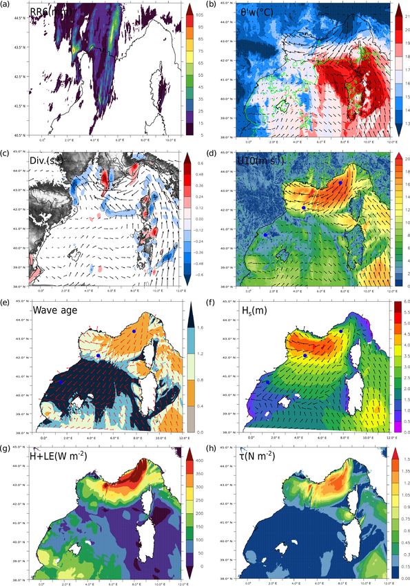
1676                 C. Sauvage et al.: Air–sea exchange mechanisms during a Mediterranean heavy precipitation event

induce variations in the atmospheric low-level dynamics and        including the surface wave effects significantly improved the
stability as well as in precipitation (e.g. Lebeaupin Brossier     simulated track as well as the intensity and the maximum
et al., 2006; Cassola et al., 2016; Stocchi and Davolio, 2017;     wind speed of the storm.
Meroni et al., 2018; Strajnar et al., 2019). How the sea sur-         The sea state evolution can be retrieved from numerical
face turbulent fluxes are formulated in the models also has a      wave model outputs and can then be used as a surface forc-
significant impact on the rainfall amounts simulated during        ing in atmospheric models. However, coupled atmosphere–
HPEs (Lebeaupin Brossier et al., 2008).                            wave systems allow one to take the feedback of the modi-
   The momentum transfer from air to ocean strongly de-            fied wind profile to the wind–wave generation into account.
pends on the sea state. In the case of wind-generated waves,       Previous studies have demonstrated the importance of wind–
the wave-induced stress represents a large fraction of the to-     wave coupling, showing significant effects on the represen-
tal stress that causes an enhancement of the drag airflow and,     tation of the atmospheric low-level dynamics (e.g. Janssen,
therefore, modifies the wind profile and the near-surface dy-      2004; Renault et al., 2012; Ricchi et al., 2016; Katsafados
namics (Janssen, 1989, 1991, 1992; Donelan, 1990). Anal-           et al., 2016; Wahle et al., 2017; Varlas et al., 2018). They
yses of in situ data highlighted the strong relationship be-       have also shown impacts on the drag coefficient over rough
tween the sea surface roughness length (z0 ) and the wave          sea and on the momentum flux resulting in a reduced sim-
age (Smith et al., 1992; Donelan et al., 1993; Drennan et al.,     ulated surface wind speed. Moreover, all of these studies
2003).                                                             have clearly reaffirmed the need for a better representation
   Nowadays, several bulk parameterizations of the sea sur-        of the sea state in the current understanding of air–sea ex-
face turbulent fluxes include this relationship between z0 and     changes. The present study investigates the impact of waves
the wave age. For example, the commonly used Coupled               on a Mediterranean HPE using a kilometric-scale coupled
Ocean–Atmosphere Response Experiment (COARE) 3.0 sea               atmosphere–wave system. The coupling involves the Wave-
surface turbulent parametrization (Fairall et al., 2003) en-       Watch III wave model and the AROME numerical weather
ables one to consider the sea state in the momentum flux           prediction model with a new flux parametrization (WASP)
parametrization – using either the formulation from Oost           that uses explicit wave parameters to compute the wave age
et al. (2002) or that from Taylor and Yelland (2001) – via         and, subsequently, the z0 and the momentum and heat fluxes.
the relationship between z0 and the Charnock coefficient. Us-      The heavy precipitation event studied here occurred from
ing the former formulation from Oost et al. (2002) in high-        12 to 14 October 2016 and had two main convective areas:
resolution numerical experiments of HPEs, Thévenot et al.          one over the sea and one that hit southern France (Hérault).
(2016) and Bouin et al. (2017) showed an impact on the lo-         Strong wind conditions and a very rough seas were observed
cation of precipitation when the sea state forcing is taken        during this event, making this case well suited for assess-
into account in the sea surface turbulent flux parametrization.    ing the influence of waves on the low-level atmosphere and
Nevertheless, these formulas are known to produce overly           heavy precipitation systems.
strong fluxes when strong winds (> 20 m s−1 ) are encoun-             A detailed description of the experimental protocol and of
tered (Pineau-Guillou et al., 2018).                               the flux parametrization is given in Sect. 2. The validation of
   Besides directly controlling the momentum flux, surface         the reference experiments against available atmospheric and
roughness also impacts the turbulent heat fluxes and the tur-      wave observations is carried out in Sect. 3. Then, in Sect. 4,
bulent structure and thickness of the atmospheric boundary         a description of the event, divided into separate phases, is
layer (Doyle, 1995, 2002). For example, an impact on the           given. Section 5 presents the results of the sensitivity analysis
thermodynamic structure and on the moisture transfer affect-       that was undertaken by comparing our different numerical
ing the evolution of a convective system has recently been         simulations. Finally, conclusions and discussions are given
shown by Varlas et al. (2018) using an air–wave coupled sys-       in Sect. 6.
tem over the Mediterranean region.
   In addition, under strong wind conditions, the intense
breaking of ocean waves occurs and generates sea spray. This       2     Numerical set-up
sea spray effect has a significant impact on the moisture and
heat transfer at the air–sea interface that has been highlighted   2.1    The atmospheric model
in several papers (e.g. Andreas, 1992; Andreas et al., 1995;
Kepert et al., 1999; Bao et al., 2000, 2011; Bianco et al.,        The non-hydrostatic AROME numerical weather prediction
2011).                                                             (NWP) model (Seity et al., 2011) is used in this study. The
   Based on this, recent studies have implemented different        AROME configuration used here is that operationally used
formulations in order to better account for the sea state and      at Météo-France with a 1.3 km horizontal resolution and a
the sea spray effect on the sea surface roughness and heat         domain centred over France, which covers our area of in-
and momentum fluxes during extreme events, such as Hurri-          terest – the north-western Mediterranean Sea (Fig. 1a). The
cane Arthur (Garg et al., 2018) or medicanes (Mediterranean        vertical grid has 90 hybrid η-levels with a first-level thick-
tropical-like cyclones; Rizza et al., 2018). They showed that      ness of almost 5 m. The time step is 50 s. In AROME,

Atmos. Chem. Phys., 20, 1675–1699, 2020                                             www.atmos-chem-phys.net/20/1675/2020/
C. Sauvage et al.: Air–sea exchange mechanisms during a Mediterranean heavy precipitation event                               1677

the advection scheme is semi-Lagrangian and the temporal          2.3     Atmosphere–wave coupling
scheme is semi-implicit. The 1.5-order turbulent kinetic en-
ergy (TKE) scheme from Cuxart et al. (2000) is used. Due to       2.3.1     Bulk iterative equations
its high resolution, the deep convection is explicitly solved
in AROME, whereas the shallow convection is solved with           The sea surface turbulent fluxes are calculated through the
the eddy diffusivity Kain–Fritsch (EDKF, Kain and Fritsch,        bulk formulae described as follows:
1990) parametrization. The ICE3 one-moment microphys-
                                                                  τ = ρCD 1U 2 ,                                                (1)
ical scheme (Pinty and Jabouille, 1998) is used to com-
pute the evolution of five hydrometeor species (rain, snow,       LE = ρLv CE 1U 1q,                                            (2)
graupel, cloud ice and cloud liquid water). The surface ex-       H = ρcpa CH 1U 1θ,                                            (3)
changes are computed by the SURFace EXternalisé (SUR-
FEX) surface model (Masson et al., 2013) that considers four      where ρ is the air density, cpa is the air heat capacity and Lv is
different surface types: land, towns, sea and inland waters       the vaporization heat constant. 1U , 1q and 1θ represent the
(lakes and rivers). Exchanges over land are computed using        air–sea gradients of velocity, specific humidity and potential
the ISBA (Interactions between Soil, Biosphere and Atmo-          temperature near the surface respectively. CD , CE and CH
sphere) parametrization (Noilhan and Planton, 1989). The          represent the transfer coefficients. Each transfer coefficient
formulation from Charnock (1955) is used for inland waters,       can be defined as follows:
whereas the Town Energy Balance (TEB) scheme is activated                   1/2 1/2
over urban surfaces (Masson, 2000). The treatment of the sea      CX = cx cd ,                                                  (4)
surface exchanges in AROME-SURFEX is detailed below
                                                                  where x is d for wind speed, θ for potential temperature and
(Sect. 2.3.1 and 2.3.2). Output fluxes are weight-averaged in-
                                                                  q for water vapour humidity. Therefore,
side each grid box according to the fraction of each respec-
tive tile, before being provided to the atmospheric model at                            1/2
                                                                   1/2                cxn
every time step.                                                  cx (ζ ) =            1/2
                                                                                                                                (5)
                                                                                      cxn
                                                                               1−      κ     ψx (ζ )
2.2   The wave model
                                                                  and
The wave model is WaveWatch III (hereafter WW3, ver-                            κ
                                                                   1/2
sion 5.16, The WAVEWATCH III Development Group,                   cxn =                ,                                        (6)
                                                                            ln(z/z0x )
2016; Tolman, 1992). The model domain covers the north-
western Mediterranean Sea at a 1/72◦ horizontal resolu-           where the subscript n refers to neutral (ζ = 0) stability, z
tion (Fig. 1b). The bathymetry is sourced from the NEMO-          refers to the reference height and ψx is an empirical func-
NWMED72 ocean model configuration described in Sauvage            tion describing the stability dependence of the mean profile;
et al. (2018b), which was originally built from the interpo-      κ is the von Karman constant.
lation of a 1/120◦ horizontal resolution topography with a           The sea surface roughness length z0 is defined by two
dedicated treatment for island, coastline and river mouth de-     terms: the Charnock’s relation (Charnock, 1955) and a vis-
lineation. The time step is 60 s.                                 cous contribution (Beljaars, 1994).
   The set of parameterizations from Ardhuin et al. (2010)
is used, as for most of the wave forecasting centres (Ard-                αch · u2∗ 0 · 11 · ν
huin et al., 2019). Thus, the swell dissipation is computed       z0 =             +           ,                                (7)
                                                                             g          u∗
with the Ardhuin et al. (2009) scheme, and the wind input
parametrization is adapted from Janssen (1991). Nonlinear         where ν is the kinematic viscosity of dry air, u∗ is the friction
wave–wave interactions are computed using the discrete in-        velocity and αch is the Charnock coefficient.
teraction approximation (DIA, Hasselmann et al., 1985). The
parametrization of the reflection by shorelines is described in   2.3.2     Wave impact on the Charnock coefficient
Ardhuin and Roland (2012). Moreover, the computation of
                                                                  One common method of coupling developing waves and
the depth-induced breaking is based on the algorithm from
                                                                  stress is to make the Charnock coefficient αch explicitly de-
Battjes and Janssen (1978), and the bottom friction formula-
                                                                  pendent on the sea state by computing it either in the wave
tion follows Ardhuin et al. (2003).
                                                                  model from the wave spectra (e.g. Janssen et al., 2001) or in
                                                                  the atmospheric model as a function of the wave age (Mahrt
                                                                  et al., 2001; Oost et al., 2002; Moon et al., 2004). Studies
                                                                  based on observations (e.g. Oost et al., 2002) express it as a
                                                                  power function:

                                                                  αch = A · χ −B ,                                              (8)

www.atmos-chem-phys.net/20/1675/2020/                                                  Atmos. Chem. Phys., 20, 1675–1699, 2020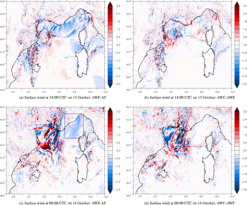
1678                    C. Sauvage et al.: Air–sea exchange mechanisms during a Mediterranean heavy precipitation event

Figure 1. Simulation domain: (a) AROME-France (topography, m) and (b) the WW3 domain illustrated with bathymetry (blue scale, m).
Black circles indicate the locations of the moored buoys, and red circles denote the locations of the surface stations (see Table 1). The satellite
track around 05:00 UTC on 12 October is shown in green, the satellite track around 18:00 UTC on 13 October is shown in yellow, the satellite
track around 05:00 UTC on 14 October is shown in magenta and the satellite track around 18:00 UTC on 14 October is shown in red and
orange – the orange track is for JASON-2 and the other tracks are for SARAL.

where coefficients A and B are either constant or depend                    ferred to the sea surface mainly sustains the wave develop-
on the surface wind speed, and the wave age χ is defined                    ment (through interaction with non-breaking waves) is be-
         c
as χ = Upa (where cp is the peak phase speed, and Ua is the                 tween 5 and 20 m s−1 . Above 20 m s−1 , the contribution of
near-surface wind). Sea state can mainly be defined using the               breaking waves to the wave stress is dominant and the wave
wave age. “Wind sea” corresponds to waves, generated by lo-                 age is not an appropriate parameter to represent the sea state
cal wind, that are still growing (wave age < 0.8) or in equi-               effect on the surface roughness. Below 5 m s−1 , under very
librium with the wind (wave age between 0.8 and 1.2) and                    weak wind conditions, the surface roughness is mainly con-
are aligned with the local wind. These waves (and only these                trolled by the viscous term (second term on the right-hand
waves) benefit from momentum transfer from the atmosphere                   side of Eq. 7). In order to reproduce these different mech-
to grow; thus, they are coupled to the wind. Conversely, swell              anisms as well as the decrease in the drag coefficient un-
(which does not depend on the momentum from the atmo-                       der very strong wind conditions, the Charnock parameter of
sphere) corresponds to waves generated by a remote or past                  the WASP parameterization is piecewise continuously de-
wind field and is characterized by a wave age above 1.2 or                  fined following Eq. (8), with the coefficients A and B be-
waves that are not aligned with the local wind.                             ing polynomial functions of the surface wind speed (see Ap-
   Assuming that the water depth is infinite (in practice, as               pendix A). Under weak to strong wind regimes where wind
soon as the depth is much larger than the dominant waves),                  stress observations are numerous and consistent with each
the phase speed of the waves can be expressed as                            other (i.e. until 23 m s−1 ), WASP has been fitted to datasets
                                                                            used to build the COARE 3.5 parameterization (Edson et al.,
       gTp
cp =       ,                                                       (9)      2013). The temperature and humidity roughness lengths z0T
       2π                                                                   and z0q (see Eq. 6), which define the corresponding neutral
where Tp is the peak period of the waves and g is the accel-                transfer coefficients, have been adjusted for the resulting sen-
eration of gravity.                                                         sible and latent heat fluxes to match the COARE 3.0 (Fairall
   Keeping the coefficients A and B constant with wind                      et al., 2003) parametrization for surface wind speeds up to
speed results in drag coefficient and wind stress values that               45 m s−1 . The stability functions ψx (Eq. 5) are a blend of
are too strong under strong wind conditions (a wind speed                   the Kansas-type functions (Businger et al., 1971) and a pro-
above 20 m s−1 ), as shown by Pineau-Guillou et al. (2018).                 file matching the asymptotic convective limit (Fairall et al.,
In order to tackle this, and to reproduce the saturation or the             1996).
decrease in the drag coefficient observed under strong to cy-                  Thus, WASP enables us to represent the Charnock parame-
clonic wind conditions (e.g. Powell et al., 2003), we take                  ter’s behaviour and its dependency on waves in a more phys-
advantage of a new parameterization called WASP (Wave-                      ical way. Moreover, it reproduces the observed decrease in
Age-dependant Stress Parametrization). This approach con-                   the drag coefficient due to very strong wind, which would
siders that the wind speed range where the wind stress trans-               not be possible using a wave-age-only Charnock parameter

Atmos. Chem. Phys., 20, 1675–1699, 2020                                                        www.atmos-chem-phys.net/20/1675/2020/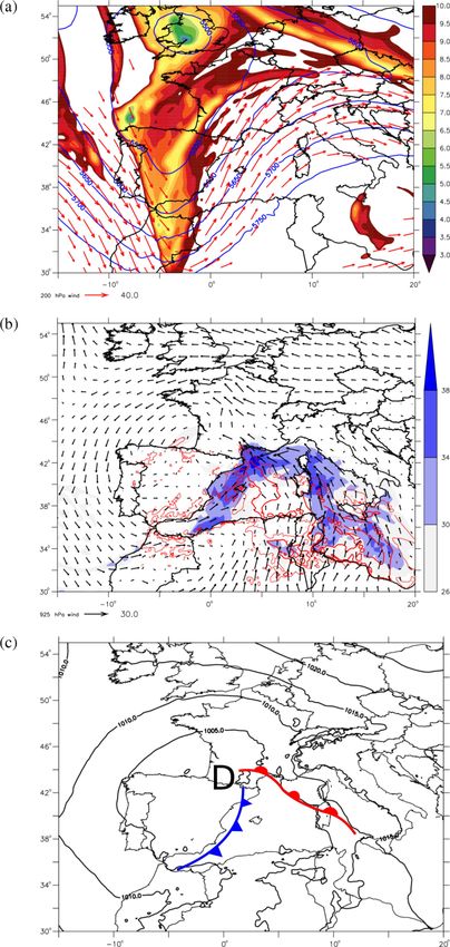
C. Sauvage et al.: Air–sea exchange mechanisms during a Mediterranean heavy precipitation event                            1679

as in Drennan et al. (2005). Therefore, WASP is more rele-         at 00:00 UTC from AROME operational analyses and that
vant for atmosphere–wave coupling and for high to very high        lasted 42 h. Hourly boundary conditions were sourced from
wind speeds.                                                       the ARPEGE (Action de Recherche Petite Echelle Grande
                                                                   Echelle, Courtier et al., 1991) operational forecasts except
2.3.3    Coupling                                                  for the SST, which came from the global daily analysis of
                                                                   the Mercator Océan International (1/12◦ resolution PSY4
The coupling is performed using the SURFEX-OASIS cou-              system, Lellouche et al., 2013). The first atmosphere-only
pling interface (Voldoire et al., 2017) that manages the ex-       (AY) simulation was carried out without any wave informa-
changes between the AROME and WW3 models. AROME-                   tion, meaning that χ was set as a function of the near-surface
SURFEX provides the two components of the near-surface             wind with Tp = 0.5 × Ua . The second atmosphere-only run
wind speed to WW3, whereas WW3 provides Tp (the peak               (AWF) was forced by the hourly wind sea Tp from the WY
period of the wind sea) to AROME-SURFEX. The OASIS                 simulation.
coupler (Craig et al., 2017) allows one to choose the coupling        Finally, a two-way coupled AROME-WW3 simulation
frequencies and the interpolation methods for the exchanged        (AWC) was undertaken following the description given in
fields.                                                            Sect. 2.3.3. The SST field and the atmospheric initial and
   Furthermore, as the AROME domain is larger than the             boundary conditions of AWC were the same as in the
WW3 domain (in particular, also covering a part of the At-         atmosphere-only simulations. Moreover, the wave boundary
lantic Ocean), there is no air–wave coupling for the ma-           conditions in AWC were the same as for WY. Wave initial
rine zones not covered by WW3 (i.e. for the grey zones in          conditions were sourced from restart files: first from WY for
Fig. 1a); thus, in these regions, χ is directly estimated in       the forecast starting at 00:00 UTC on 12 October, and then
WASP as a function of wind with Tp = 0.5 × Ua and, in turn,        from the previous AWC forecast run for the following days
                                                       cp
cp = gU  a
       4π . This can be found using the relation Tp = g × Ua ,
                                                                   (after 24 h). The coupling frequency was set to 1 h in both
where cp is approximately 5 for a typical nondimensional           directions. Each exchanged field was interpolated using a bi-
fetch and the gravity constant, g, is approximately 10.            linear method.

2.4     Set of simulations
                                                                   3     Validation of the experiments
In this study, three kinds of simulations were examined:
wave-only, atmosphere-only and wave–atmosphere coupled             3.1    Available observations
simulations. As the objective of this study is to better assess
the role of the waves on the dynamics (i.e. the impact on the      In order to validate the simulations, we collected several
momentum flux and surface wind) as well as the impact on           observations of the surface and near-surface in the north-
the sea surface turbulent heat fluxes, a common and fixed sea      western Mediterranean area (see Fig. 1b, which displays the
surface temperature (SST) is used in all the experiments and       observations over the WW3 domain).
no ocean coupling is introduced so that the wave effects on           Data from 14 moored buoys (listed in Table 1 and plot-
these fluxes are not masked.                                       ted in Fig. 1b), available either from the Copernicus Marine
   First a wave-only simulation (named WY) was run. For            Environment Monitoring Service (CMEMS, http://marine.
this simulation, WW3 ran from 5 to 15 October 2016 with            copernicus.eu/, last access: 3 Feruary 2020) database or from
the initial conditions (Hs , Tp ) set to zero and a near-surface   the HyMeX programme database (http://mistrals.sedoo.fr/
wind forcing sourced from AROME forecasts at an hourly             HyMeX/, last access: 3 Feruary 2020), were first used for
frequency (+1 to +24 h each day, see Sauvage et al., 2018a).       validation. These platforms measure a wide variety of near-
The period from 5 to 12 October served here as a spin-up           surface variables that may include sea temperature, salinity
period and will not be considered in the following. Bound-         and wave parameters, such as the significant wave height
ary conditions for the wave model consisted of eight spectral      (Hs ) and peak period (Tp ), as well as some atmospheric pa-
points distributed along the domain and provided by a WW3          rameters, such as the 2 m air temperature, relative humidity,
global 1/2◦ resolution simulation run at Ifremer (Rascle and       the 10 m wind speed, wind direction and gusts. In addition
Ardhuin, 2013). These points (each defined following 24 di-        to these buoys, six coastal surface weather stations from the
rections and 31 frequencies) were chosen as close to our do-       Météo-France network were used (mainly around the Gulf of
main border as possible from the output points available from      Lion and in Corsica) in order to complete the coverage over
the WW3 global simulation. They were then linearly interpo-        the area of interest with respect to atmospheric in situ data.
lated onto our grid (1/72◦ ) in the WW3 preprocessing rou-         Altimetric data from two satellites crossing the area during
tine.                                                              the event were used for the significant wave height valida-
   Atmosphere-only simulations were carried out with               tion. The first satellite was Jason-2 (OSTM/Jason-2 Products
AROME. Each AROME simulation was composed of fore-                 Handbook, 2008) from the joint CNES/NASA oceanogra-
cast runs that started every day (12, 13 and 14 October 2016)      phy mission Jason. The altimetric measurements used were

www.atmos-chem-phys.net/20/1675/2020/                                               Atmos. Chem. Phys., 20, 1675–1699, 2020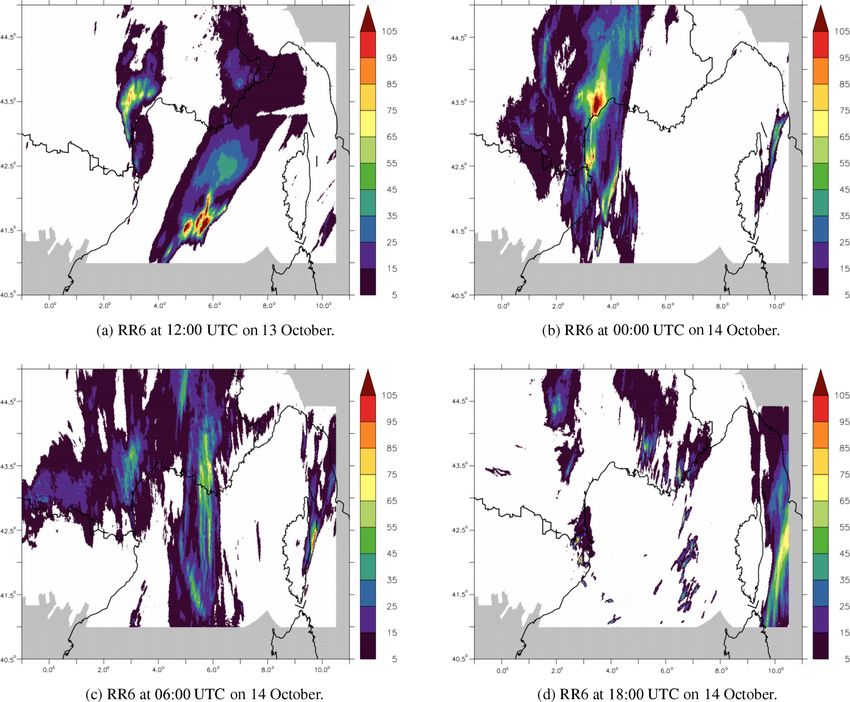
1680                  C. Sauvage et al.: Air–sea exchange mechanisms during a Mediterranean heavy precipitation event

Table 1. Names and locations of the moored buoys and surface stations (in italics) used for validation. The numbers given in front of the
names refer to Fig. 1b.

        Name                 Longitude    Latitude    Source           Name               Longitude    Latitude    Source
        1-Lion               4.7◦ E       42.1◦ N     Météo-France     11-Leucate         3.13◦ E      42.92◦ N    CMEMS
        2-Azur               7.8◦ E       43.4◦ N     Météo-France     12-MESURHO         4.87◦ E      43.32◦ N    CMEMS
        3-Tarragona          1.47◦ E      40.68◦ N    CMEMS            13-Le Planier      5.23◦ E      43.21◦ N    CMEMS
        4-Begur              3.65◦ E      41.92◦ N    CMEMS            14-Barcelone       2.2◦ E       41.32◦ N    CMEMS
        5-Valence            0.20◦ E      39.52◦ N    CMEMS            1-Leucate          3.06◦ E      42.92◦ N    Météo-France
        6-Dragonera          2.1◦ E       39.56◦ N    CMEMS            2-Sète             3.69◦ E      43.4◦ N     Météo-France
        7-Bahia de Palma     2.7◦ E       39.49◦ N    CMEMS            3-Hyères           6.15◦ E      43.1◦ N     Météo-France
        8-Canal de Ibiza     0.78◦ E      38.82◦ N    CMEMS            4-Martigues        5.05◦ E      43.33◦ N    Météo-France
        9-Banyuls-sur-mer    3.17◦ E      42.49◦ N    CMEMS            5-Bonifacio        9.18◦ W      41.37◦ N    Météo-France
        10-Sète              3.78◦ E      43.37◦ N    CMEMS            6-Ersa             9.36◦ W      43◦ N       Météo-France

the Geophysical Data Record (GDR) from the MLE4 (maxi-                 ferent regions, i.e. the Gulf of Lion and the Balearic Sea,
mum likelihood estimator) altimeters’ retracking algorithm             some differences can be highlighted. In the Gulf of Lion and
that were corrected following a buoy comparison method:                along the French Riviera, a correlation coefficient of 0.82
Hs _cor = 1.0149 × Hs + 0.0277. The second dataset was ob-             was found. Looking at the buoys located in the Balearic Sea,
tained from GDR data from the SARAL/AltiKa satellite                   i.e. where the wind was weaker, the simulation represents the
(SARAL/AltiKa Products handbook, 2013) that also uses the              wind speed value well but a low correlation (0.45) is found.
MLE4 altimeters’ retracking algorithm but simply removes                  By looking at the French western coastal buoys in more
erroneous Hs using a threshold relationship. Both satellites           detail, such as Leucate (Fig. 2) which is located on the most
combined gathered 292 measures of Hs during the period be-             western part of the Gulf of Lion, a large underestimation of
tween 12 and 14 October 2016.                                          the wind speed was found. The observed wind speed reached
   To validate the rainfall accumulation, the ANTILOPE                 values of between 18 and 20 m s−1 several times, whereas the
product from Météo-France was used (Laurantin, 2008). This             simulation only reached 15 m s−1 . In addition, at Sète, the
product merges rain gauges and radar data. This analysis was           wind intensity was in good agreement but decreased faster
complemented by the use of the Météo-France radar compos-              than observed (not shown). There is also a delay at the end
ite images over western Europe.                                        of the event between the simulation and observations, which
                                                                       is notable at the Lion buoy (Fig. 2) when a transition to a
3.2    Validation of AWF and WY                                        northerly wind occurred.
                                                                          The validation against in situ data for the 2 m air temper-
For the validation of our wave and atmospheric reference               ature (T2M) and relative humidity (RH) (Table 2) showed
simulations, WY and AWF respectively, the time series from             that AWF represented these two atmospheric parameters
12 to 14 October were built using the first 24 h of simula-            quite well with correlation coefficients of 0.68 and 0.78 re-
tion starting each day (Fig. 2). Observations and simulations          spectively, despite small overestimations (averaged biases of
were compared using the nearest grid point in space and time           0.26 ◦ C and 2.23 % respectively). These scores, along with
from the model (WW3 or AROME) to the observation grid                  the validation against low-level wind and wave parameters,
point. The bias, the root-mean-square error (RMSE) and the             gave us confidence in the use of AWF with respect to inves-
correlation were computed and are summarized in Table 2.               tigating the evolution of the turbulent fluxes at the air–sea
   During the entire event, the sea state appeared to be well          interface during the abovementioned HPE.
represented by WY with a correlation of 0.90 for Hs and Tp .
Looking at Fig. 2, Hs and Tp seemed to be underestimated
during the event. This was confirmed by a negatives bias of            4   Event description
−23 cm for Hs and −0.79 s for Tp as well as by the compari-
son of the simulated Hs against satellite data that showed an          The HPE studied occurred between the 13 and 14 Octo-
average bias of about −0.17 cm (Table 2). However, a good              ber 2016 over the north-western Mediterranean Sea. This
correlation of 0.78 was obtained with satellite data.                  event could be defined as a typical “Cyclonic Southerly”
   In AWF, the wind speed and direction were quite well rep-           (CS), following the four classifications of synoptic types
resented with correlations of 0.64 and 0.86 respectively (Ta-          from Nuissier et al. (2011). Indeed, the synoptic meteoro-
ble 2), although they were very slightly overestimated dur-            logical situation (Fig. 3) was characterized by a trough at al-
ing the event with an averaged bias of 0.04 m s−1 and 2◦ re-           titude extending from the British Islands to Spain and associ-
spectively. Looking at the wind speed correlation over dif-            ated with a lowering of the tropopause (Fig. 3a) that induced

Atmos. Chem. Phys., 20, 1675–1699, 2020                                                  www.atmos-chem-phys.net/20/1675/2020/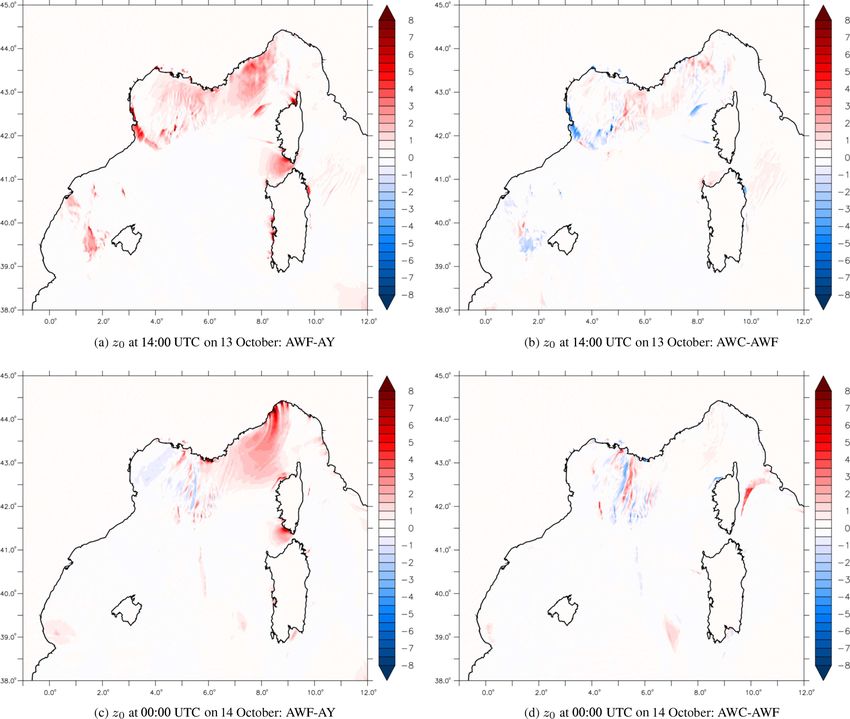
C. Sauvage et al.: Air–sea exchange mechanisms during a Mediterranean heavy precipitation event                                      1681

Table 2. Skill scores computed against surface stations and satellite data for the wave-only simulation (WY) and the coupled simulation
(AWC) for wave parameters (Hs , Tp ) and for the atmosphere-only simulations (AY and AWF) and coupled simulations (AWC) for atmo-
spheric parameters. WSP represents 10 m wind speed (m s−1 ), WDIR represents 10 m wind direction (◦ ), T2m represents 2 m air temperature
(◦ C) and RH2M represents 2 m relative humidity (%).

                                                          Moored buoys and surface stations
                          WY                             AY                              AWF                          AWC
  Parameter     Bias   RMSE     Correlation   Bias   RMSE     Correlation   Bias       RMSE    Correlation    Bias   RMSE    Correlation
  Hs          −0.23      0.53         0.90       –        –            –       –           –            –    −0.28    0.58         0.90
  Tp          −0.79      1.16         0.90       –        –            –       –           –            –    −1.27    1.64         0.88
  WSP             –         –            –    0.22     2.70         0.66    0.04        2.75         0.64     0.09    2.67         0.65
  WDIR            –         –            –    1.43    42.05         0.85     2.0       42.46         0.86     1.85   42.95         0.85
  T2M             –         –            –    0.39     1.25         0.70    0.45        1.32         0.66     0.44    1.32         0.66
  RH2M            –         –            –    2.19     8.84         0.79    2.89        9.66         0.76      3.0    9.97         0.76
                                                                      Satellites
  Hs           -0.17      0.4         0.78      –         –            –           –      –             –    −0.28     0.5         0.71

Figure 2. Evolution of Hs (m), Tp (s), wind speed (m s−1 ) and wind direction (◦ ) simulated with AWF–WY (green), AWC (red) and AY
(blue) against buoy observations (black triangles).

a south-westerly flow over south-eastern France. A cyclonic            cold and warm fronts (Fig. 3c), and the low-level flow also
circulation took place at low levels (Fig. 3b) with a high             shifted eastwards.
moisture content over the Gulf of Lion and a strong south-                The HPE was characterized by four periods that can be
easterly flow that originated from south-eastern Tunisia. Dur-         distinguished using observations over land and the refer-
ing the night and the following day, the trough moved east-            ence simulation (AWF) for the marine low-level conditions:
wards from the Bay of Biscay to the Gulf of Lion along with            (i) initiation stage, (ii) mature systems, (iii) north-eastward

www.atmos-chem-phys.net/20/1675/2020/                                                      Atmos. Chem. Phys., 20, 1675–1699, 2020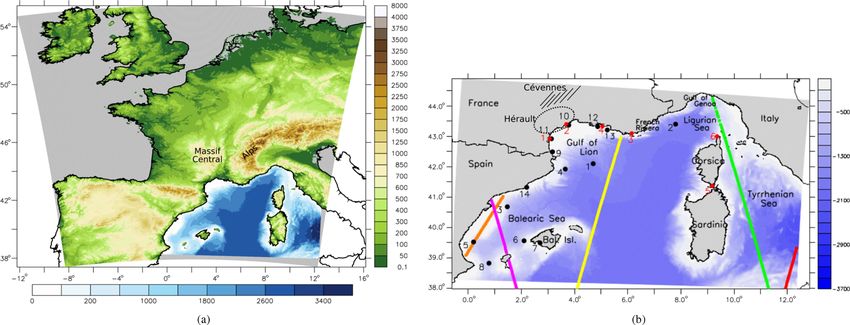
1682                   C. Sauvage et al.: Air–sea exchange mechanisms during a Mediterranean heavy precipitation event

                                                                         propagation and (iv) tramontane wind onset. In the follow-
                                                                         ing, a detailed description of the chronology of the event and
                                                                         the mechanisms involved is carried out. For this purpose, the
                                                                         42 h forecast starting at 00:00 UTC on 13 October 2016 from
                                                                         AWF was used along with observations.

                                                                         4.1   Chronology of the convective systems

                                                                         Phase I, from 03:00 to 18:00 UTC on 13 October 2016 (+3
                                                                         to +18 h in the simulation), was marked by the triggering
                                                                         of deep convection and the stationarity of the two main sys-
                                                                         tems. The first deep convective system was triggered in the
                                                                         Cévennes foothills, south of the Massif Central, (Figs. 1, 4a,
                                                                         5a), where the unstable rapid south-easterly marine flow en-
                                                                         countered orography (Fig. 5c). The second deep convection
                                                                         system was a MCS associated with large precipitation over
                                                                         the sea (Figs. 4a, 5a). It formed at the convergence between
                                                                         the warm south-easterly flow, associated with high CAPE
                                                                         values, and the colder and drier easterly flow from the Alps
                                                                         and Ligurian Sea (Fig. 5c, d). These two convective systems
                                                                         were well represented in the reference simulation (Figs. 4a,
                                                                         5a) in terms of location and rainfall amounts compared to
                                                                         observations. The simulated radar reflectivities also corre-
                                                                         sponded quite well to observations (not shown) except in
                                                                         north-eastern Spain where overly active convective systems
                                                                         were simulated.
                                                                            During Phase II, from 19:00 UTC on 13 October to
                                                                         03:00 UTC on 14 October (+19 to +27 h in the simula-
                                                                         tion), the precipitating system over the Hérault region re-
                                                                         mained stationary. Its intensity increased in the observations
                                                                         (Fig. 4b), whereas precipitation totals for the second system
                                                                         over the sea decreased. In AWF, the simulated precipitating
                                                                         system over the sea started to shift towards the east, while
                                                                         precipitation over the Hérault region decreased (Fig. 6a).
                                                                         The simulated cold front progressed eastwards earlier than in
                                                                         the observations; thus, the southern flow also started to shift
                                                                         (Fig. 6d) as did the convergence line over the sea (Fig. 6c).
                                                                            Phase III, from 04:00 to 10:00 UTC on 14 October (+28 to
                                                                         +34 h in the simulation), was marked by the north-eastward
                                                                         propagation of the system. As the western front was mov-
                                                                         ing eastwards, the system over the Hérault region shifted
                                                                         toward the French Riviera (Fig. 7c), leading to a local de-
                                                                         crease in the precipitation total (< 60 mm over the Hérault
                                                                         region, Fig. 4c). In the simulation, the system over the sea
Figure 3. Synoptic situation at 12:00 UTC on 13 October 2016 from        also moved eastwards, extending from west of Corsica to
the ARPEGE analysis (a) at high level: the coloured shading is the       the French Riviera, and there was a decrease in the rain-
height of the 2 PVU (potential vorticity units) isosurface (km), the     fall amounts (Fig. 7a). It appeared that the simulated east-
blue contours are the geopotential height (m) at 500 hPa and the red     ward propagation was earlier than observed. The southerly
arrows denote the wind above 20 m s−1 at 200 hPa. Synoptic situa-        flow was also consistently shifted and was located between
tion at 12:00 UTC on 13 October 2016 from the ARPEGE analysis
                                                                         Corsica–Sardinia and continental Italy (Fig. 7d) with a main
(b) at low level: the coloured shading is the integrating water vapour
                                                                         convergence area over the Ligurian Sea. At the same time, the
(kg m−2 ), the red contours are the convective available potential
energy (J kg−1 ) and the black arrows denote the wind at 925 hPa.        intensity of the inland system (over the Hérault region) was
Panel (c) shows the mean sea level pressure (black contours) and         overestimated compared with observations (Figs. 4c, 7a).
position of the cold (blue) and warm (red) fronts.                          The last phase (Phase IV), from 11:00 UTC on 14 Octo-
                                                                         ber (+35 h to the end of simulation, not shown), was charac-

Atmos. Chem. Phys., 20, 1675–1699, 2020                                                   www.atmos-chem-phys.net/20/1675/2020/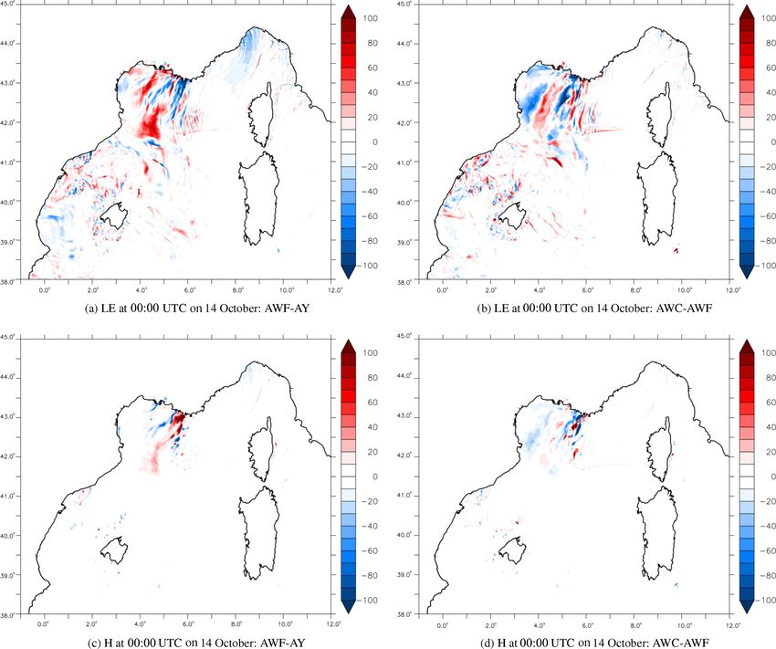
C. Sauvage et al.: Air–sea exchange mechanisms during a Mediterranean heavy precipitation event                           1683

Figure 4. The 6 h rainfall amounts (mm) from ANTILOPE observations.

terized by the end of the precipitation over France (Fig. 4d)           the event, first aligned with the south-easterly wind in
and the beginning of a new wind regime in the Gulf of Lion,             Phase I and then crossed, as wind and waves were op-
with a dry and cold north-westerly flow corresponding to the            posite.
regional tramontane wind regime. Thus, the warm southern
flow was limited to the south-east of the simulation domain           – The Lion buoy was located where the easterly wind was
and fed the precipitating system located from the northern              stronger during Phase I, generating a young wind sea
Sardinian region to continental Italy (Fig. 4d). For this pe-           with strong Hs . It evolved to a well-developed wind sea
riod, the simulation was in good agreement with observations            during Phase II and then to a swell as the fetch became
in term of rainfall locations and amounts.                              longer in this area.
                                                                      – The Azur buoy was located in the strong easterly wind
4.2   Evolution of the sea state                                        throughout the event. Characterized by a short fetch, a
                                                                        wind sea was continuously produced in this area.
Three different areas can be distinguished in our domain,
mainly represented by the three moored buoys (Fig. 1, Ta-           During Phase I, a strong easterly wind (between 15 and
ble 1).                                                           20 m s−1 ; Figs. 2, 5b) affected the Ligurian Sea, from the
                                                                  French Riviera to the Gulf of Lion. This created a wind
  – The Tarragona buoy, where the wind was weak, was sit-         sea, with young waves (see the Azur buoy in Figs. 5e and
    uated in a long fetch area. There was swell throughout        8) aligned with the wind and associated with moderate Hs

www.atmos-chem-phys.net/20/1675/2020/                                              Atmos. Chem. Phys., 20, 1675–1699, 2020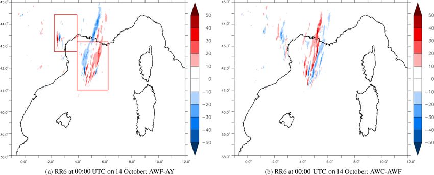
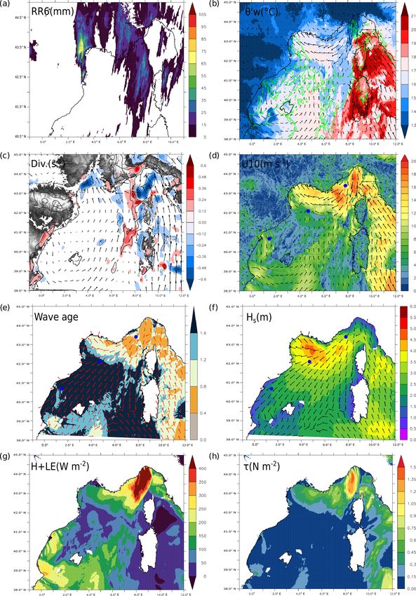
1684                   C. Sauvage et al.: Air–sea exchange mechanisms during a Mediterranean heavy precipitation event

Figure 5. (a) The 6 h rainfall amount (mm). (b) The pseudo-adiabatic potential temperature θw ’ (coloured shading, ◦ C) and wind (m s−1 ,
arrows) at 925 hPa with the CAPE over 750 J kg−1 shown using green contours. (c) The wind divergence (coloured shading, 10−3 s−1 ,
values between -0.12 and 0.12 are masked) at 950 hPa, where the black contours are the vertical velocity (Pa s−1 ) at 950 hPa and the black
arrows are the horizontal winds (m s−1 ). (d) The 10 m wind intensity and direction (m s−1 ). (e) The wave age and wave direction. (f) The
wave significant height (m) and wave direction. (g) The total turbulent heat fluxes (H , LE) (W m−2 ). (h) The wind stress (N m−2 ) simulated
by AWF at 12:00 UTC on 13 October. Blue dots in (d), (e) and (f) represent the Tarragona, Lion and Azur buoys (from west to east).

Atmos. Chem. Phys., 20, 1675–1699, 2020                                                    www.atmos-chem-phys.net/20/1675/2020/
C. Sauvage et al.: Air–sea exchange mechanisms during a Mediterranean heavy precipitation event            1685

Figure 6. Same as for Fig. 5 but at 00:00 UTC on 14 October.

www.atmos-chem-phys.net/20/1675/2020/                                    Atmos. Chem. Phys., 20, 1675–1699, 2020
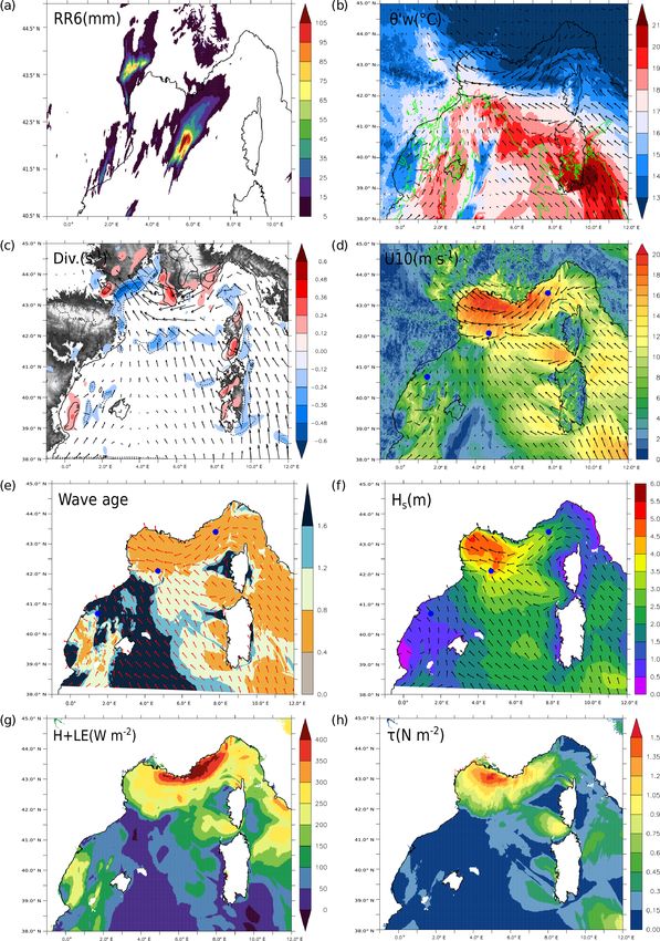
1686                  C. Sauvage et al.: Air–sea exchange mechanisms during a Mediterranean heavy precipitation event

Figure 7. Same as for Fig. 5 but at 06:00 UTC on 14 October.

Atmos. Chem. Phys., 20, 1675–1699, 2020                                      www.atmos-chem-phys.net/20/1675/2020/
C. Sauvage et al.: Air–sea exchange mechanisms during a Mediterranean heavy precipitation event                             1687

(< 3 m, Fig. 5f). In fact, the waves in this area were directly   (over 300 W m−2 , Fig. 5g). In addition, this region was char-
generated by the local wind throughout the event (Fig. 8)         acterized by the strongest humidity transport, due to the east-
with low wave age values (< 1) and a similar direction be-        erly flow, towards the Gulf of Lion as the air humidity in-
tween wind and waves. In the Gulf of Lion, a rough to             creased (over 94 %). Under a strong easterly wind, along the
very rough sea was observed (Hs ∼ 4–5 m) that was asso-           French Riviera, the difference between SST and T2M was up
ciated with a Tp of about 8 s (Fig. 2). Still, a weak wave age    to 4 ◦ C (5 ◦ C locally) and, thus, with high sensible heat flux
(Figs. 5e, 8) was found here due to strong winds. Thus, the       (H ) values (over 150 W m−2 , Fig. 5g). The warm (> 23 ◦ C)
waves in this area were mainly generated by the wind above.       and humid (over 85 %) southern flow did not produce large
   In the Balearic Sea high wave ages were simulated (> 1.2,      heat fluxes (Fig. 5g). It can be noticed that there was warm
Fig. 8) under a weak south-westerly flow (Fig. 2); this in-       and dry air masses in the Balearic Sea, but the weak south-
duced a weaker Hs , which corresponded to a moderate sea.         westerly wind blowing in this area limited evaporation and
The sea state in this area was consistent with a swell coming     heat fluxes. The momentum flux was the largest under the
from the south.                                                   strong easterly wind in the Gulf of Lion – reaching up to
   During Phase II, Tp reached a maximum (∼ 10 s observed)        1.5 N m−2 , whereas it reached up to 1.2 N m−2 locally un-
in the Gulf of Lion; Hs values were also highest in this re-      der the south-easterly flow (Fig. 5h). It remained lower than
gion (about 6 m), corresponding to a very rough sea which         0.3 N m−2 throughout the rest of the domain.
is rather exceptional in the Mediterranean Sea. This well-           As the system moved eastwards during Phase II, the rapid
developed wind sea (wave age between 0.8 and 1.2) was             low-level flow moved from the Gulf of Lion to the Ligurian
due to the continuous easterly wind that had been blowing         Sea. The evaporation kept increasing in this area, and the dry
since Phase I (Figs. 2, 6b). The intensity of the easterly flow   air in the Gulf of Genoa became almost saturated in the Gulf
decreased in the Gulf of Lion but increased in the Ligurian       of Lion. The largest values of the momentum flux were lo-
Sea (±2–3 m s−1 ; Figs. 2, 6b). In the Balearic Sea, the wave     cated along the French Riviera at this time (Fig. 6h). LE
ages were still high but the wave direction changed progres-      decreased by more than 50 W m−2 in the Gulf of Lion and
sively from easterly to north-easterly. This corresponded to      increased along the French Riviera and the Gulf of Genoa,
the swell coming from the Ligurian Sea, as a weak south           reaching more than 360 W m−2 (Fig. 6g). As the cold front
to north-westerly wind (< 10 m s−1 ) was blowing locally          was shifting, the low-level air mass in the Balearic became
(Figs. 2, 6b, e, 8).                                              drier and pushed the humid southerly flow to the east. The
   During Phase III, Hs started to decrease over the domain       highest values of H were also shifted in the Gulf of Genoa
(Figs. 2, 7f) and the observed Tp reached a maximum in the        and reached 200 W m−2 (Fig. 6g), whereas H significantly
Balearic Sea and in the western part of the Gulf of Lion,         decreased in the Gulf of Lion.
which was associated with swell (Figs. 2, 7e, 8). As the front       During Phase III, drier air (RH < 70 %) was located from
moved eastwards, a significant decrease in the easterly wind      the Balearic Sea to the coast of Sardinia. In the Gulf of Lion,
was observed (up to −7 m s−1 ; Figs. 2, 7b), whereas the wind     low-level air continued to get drier, whereas moist air was
speed was strongest in the Gulf of Genoa. Indeed, the wind in     now mainly located along the French Riviera and in the Gulf
the Gulf of Lion started to change direction with a transition    of Genoa (where precipitation occurred). Under precipita-
to a northerly wind (see Leucate, Sète and Lion in Fig. 2). As    tion, H increased to 250 W m−2 (Fig. 7g). LE significantly
in the Balearic Sea (Figs. 7e, 8), the wind changed direction     decreased by 100 W m−2 along the French Riviera but was
from north-westerly to westerly.                                  still highest in the Gulf of Genoa (Fig. 7g). A large decrease
   Finally, during Phase IV, Hs kept decreasing over the do-      (of 1 N m−2 ) was also noticed in the momentum flux along
main (< 3 m, Fig. 2). Tp significantly decreased in the Gulf      the French Riviera and maximum values were found in the
of Lion, whereas the highest values were still located in the     Gulf of Genoa (Fig. 7h).
Balearic Sea (Fig. 2). At both locations, the swell generated        During the last phase (Phase IV), with the large decrease
along the French Riviera was present (Fig. 8), while the east-    in the wind intensity and the precipitation now located over
erly wind significantly decreased (now < 14 m s−1 , Fig. 2).      Italy, RH decreased along the French Riviera and in the Gulf
The onset of a north-westerly wind (Tramontane) in the Gulf       of Genoa in association with a large decrease (of 150 W m2 )
of Lion was observed (Fig. 2), while a westerly wind was          in the heat fluxes. The momentum flux was lower than
blowing over the Balearic Sea.                                    0.3 N m−2 in the Gulf of Genoa at this time.
                                                                     A rapid analysis of the relationship between the heat fluxes
4.3   Air–sea interface                                           (H and LE) and atmospheric parameters (Ua , temperature
                                                                  gradient, humidity gradient) was carried out using scatter-
The latent heat flux (LE) was quite low over the domain, as       plots (not shown). It highlighted that the sensible heat flux
displayed by Fig. 5g. During Phase I, the cold and dry air        was more correlated with the temperature gradient at the air–
from the Alps became rapidly warmer and more humid as             sea interface (0.56), which was related to the cold air present
it flowed westwards over the sea. Evaporation started in this     in the easterly flow or below precipitation. Conversely, the la-
area and also marked the location of the largest LE values        tent heat flux was more correlated with the wind (0.49) than

www.atmos-chem-phys.net/20/1675/2020/                                              Atmos. Chem. Phys., 20, 1675–1699, 2020
1688 C. Sauvage et al.: Air–sea exchange mechanisms during a Mediterranean heavy precipitation event
Figure 8. Evolution of the wave age (blue) and direction (◦ ) of local wind (red) and waves (black) simulated with AWF (WY) during the
13 October run at three different moored buoys. Orange lines limit the four different phases (I, II, III and IV).
with the gradient of humidity (0.31). In summary, the maxi- and the effects of waves on the HPE in a continuous way
mum turbulent fluxes were associated with the easterly low- during these two phases, the sensitivity analysis was carried
level jet due to strong winds and large air–sea temperature out considering the 42 h of forecast starting at 00:00 UTC on
(moisture) gradients for heat fluxes. In the southerly flow, 13 October.
heat fluxes appeared more limited despite moderate wind.
This highlighted the role of the Ligurian easterly flow in ex- 5.1 Low-level flow
tracting heat and moisture from the sea and in providing them
to the MCSs. 5.1.1 Impact of the waves: AWF versus AY
Finally, looking at the different phases of the event, some
areas emerged as potential regions where the waves should In the following, AWF, which takes the sea state into account,
have an impact on the low-level flow. Indeed, during phases is compared to the atmosphere-only simulation, AY (see
I and II, an effect on the momentum flux was expected in ar- Sect. 2.4). Figure 9a and c present the difference in the sea
eas of strong easterly wind and of wind sea, especially over surface roughness length (z0 ) between AWF and AY. Dur-
the French Riviera and the Gulf of Lion in Phase I. These ing Phase I, an increase in z0 (from 2 × 10⁻³ to 4 × 10⁻³ m)
regions were also the places with the highest heat fluxes dur- in AWF was found (compared with AY) over the wind sea
ing the event and, thus, were more likely to be affected by under a strong easterly wind in the Gulf of Lion and along
the sea state. Therefore, the sensitivity to the impact of the the French Riviera. Throughout the rest of the domain, much
representation of sea state will be particularly investigated in smaller z0 differences were noticed (less than 2 × 10⁻⁴ m).
these areas in the following. These changes induced an increase in the drag coefficient Cd
of up to 0.8 × 10⁻³ and led to an increase in the momen-
tum flux of more than 0.1 N m2 . Finally, this increase in the
5 Sensitivity analysis momentum flux resulted in a decrease of more than 1 m s−1
in the 10m wind speed intensity of the strong easterly flow
In this section, the goal is to better understand the impact of over a large area between the Gulf of Lion and the French
the waves on the sea surface turbulent fluxes and to evaluate Riviera (Fig. 10a). During Phase II, along the French Riviera
the impact on the HPE forecast. We focused on phases I and and the Gulf of Genoa, characterized by the strong easterly
II, at 14:00 UTC on 13 October and 00:00 UTC on 14 Oc- wind and a young wind sea (Fig. 6b, e), z0 increased by more
tober 2016, respectively (corresponding to +14 and +24 h than 2×10⁻³ m and up to 1×10⁻² m in AWF compared with
of forecast respectively, starting at 00:00 UTC 13 October). AY (Fig. 9c). Knowing that z0 barely exceeds 3 × 10⁻³ m in
In order to examine the mechanisms at the air–sea interface AY, these differences correspond to an increase of more than
Atmos. Chem. Phys., 20, 1675–1699, 2020 www.atmos-chem-phys.net/20/1675/2020/C. Sauvage et al.: Air–sea exchange mechanisms during a Mediterranean heavy precipitation event 1689 Figure 9. z0 (10−3 m) differences at 14:00 UTC on 13 October (a, b) and at 00:00 UTC on 14 October (c, d) between AWF–AY (a, c) and AWC–AWF (b, d). 100 % of the values in AY. Under the convective system some space and time. Thus, the results confirmed the primary ef- difference dipoles were found. In the Gulf of Lion, a slight fect of the representation of sea state as notably highlighted increase in z0 was seen. While differences in z0 in Liguria by Thévenot et al. (2016) and Bouin et al. (2017): when the were observed from the beginning of the simulation, differ- sea state is taken into account, an increased surface rough- ences under the MCS and in the Gulf of Lion appeared to re- ness and wind stress are observed that slow down the up- sult from differences in the movement of the convective sys- stream low-level flow. tem over the sea, which were induced by the decrease in the In the two subareas delineated in Fig. 10c, it was found wind intensity during Phase I. Due to the same mechanisms that, on average, a slowdown of the 10 m wind speed was as in Phase I, the increase in z0 upstream of the MCS (i.e. obtained in both areas during the four phases. Specifically, along the French Riviera) directly impacted the Cd , which an averaged slowdown of 0.9 m s−1 was noticed in the Gulf increases in AWF by 0.2 × 10⁻³ to more than 1 × 10⁻³ lo- of Lion during the Phase I. This represented a decrease of cally. This led to an increase in the wind stress of between about 6 % of the average wind intensity in AWF. The same 0.1 and 0.3 N m2 in this area and resulted in a slowdown of result was found during Phase II along the French Riviera between 1 and 2 m s−1 the 10 m in the wind speed along the with an average decrease of 0.9 m s−1 (−7 %). Scores did French Riviera (Fig. 10c). Larger differences were found un- not appear to be change significantly between AWF and AY der the convective system but appeared inhomogeneous in (Table 2). However, a lower bias in the wind intensity was www.atmos-chem-phys.net/20/1675/2020/ Atmos. Chem. Phys., 20, 1675–1699, 2020
1690                  C. Sauvage et al.: Air–sea exchange mechanisms during a Mediterranean heavy precipitation event

Figure 10. Surface wind (m s−1 ) differences at 14:00 UTC on 13 October (a, b) and at 00:00 UTC on 14 October (c, d) between AWF–AY (a,
c) and AWC–AWF (b, d).

found (0.04 m s−1 in AWF compared with 0.22 m s−1 in AY)              waves. Differences in the sensible heat flux (Fig. 11c) were
and was actually mostly due to a large improvement at the             mainly located under the precipitation with very weak differ-
Azur buoy, where the bias was reduced from 0.42 m s−1 in              ences along the French Riviera.
AY to 0.08 m s−1 in AWF.
   Figure 11a and c present the heat flux (the latent and sen-        5.1.2   Impact of the coupled system: AWF versus AWC
sible fluxes respectively) differences between AWF and AY.
Along the French Riviera, where the latent heat flux was the          Figure 9b and d present the differences in z0 between AWF
strongest, a decrease was obtained in AWF during phases               and the atmosphere–wave coupled system AWC. During
I and II. However, this corresponded to a small decrease              Phase I, z0 in AWC increased by up to 2 × 10⁻³ m over
(5 W m−2 on average) that was equivalent to 2 % of the to-            the French Riviera and the eastern part of the Gulf of Lion
tal averaged latent flux. Relatively larger differences, both         (Fig. 9b). As a result, a slight decrease in the 10 m wind speed
positive and negative, were found under the convective sys-           intensity was found in this region, about 0.6 m s−1 (Fig. 10b).
tem. However, on average, these differences were small, rep-          During Phase II, smaller differences were obtained along the
resenting ±2 % (3 W m−2 ). They were very likely related to           French Riviera. This corresponded to a small increase in z0
differences in terms of the intensity of the convection within        in AWC of about 1 × 10⁻³ m under a strong easterly wind
the MCS and its location and were not a direct effect of the          (Fig. 9d). The 10 m wind speed was decreased in AWC by
                                                                      no more than 0.3 m s−1 (Fig. 10d). The smaller impact on

Atmos. Chem. Phys., 20, 1675–1699, 2020                                                 www.atmos-chem-phys.net/20/1675/2020/
C. Sauvage et al.: Air–sea exchange mechanisms during a Mediterranean heavy precipitation event 1691
Figure 11. (a, b) LE (W m−2 ) and (c, d) H (W m−2 ) differences at 00:00 UTC on 14 October between AWF–AY (a, c) and AWC–AWF (b,
d).
the low-level dynamics in AWC can be explained by the have been induced by the movement and the convective cell
feedback of the wind on the waves. Indeed, on average, it evolution of the MCS.
was found that Hs was decreased by 12 % and Tp by 7 % in Thus, on average, coupling only showed minor effects on
AWC during the event. As we already had an underestima- the dynamics and on the heat and moisture exchanges below
tion of the wave parameters in WY, this decrease in AWC in- the upstream low-level flow. One main explanation for this
duced larger biases (Table 2). Larger differences in the wind small effect might be that the waves used in AWF and AWC
intensity were also found under the convective system and were really close to each other in term of spatial and tempo-
downstream of it in the Gulf of Lion (Fig. 10d). However, ral resolution, both simulated using WW3. Locally, effects
these were not really consistent throughout the simulation on the dynamics can be significant; this is especially true in
and were mainly due to the movement of the system and the strong wind and wind sea areas, where we found a decrease
slowdown of the wind during Phase I. in the wind speed and in Hs and Tp .
Figure 11b and d illustrate the differences in the heat
fluxes. Very small variations were noticed for either LE or 5.2 Precipitation
H (less than 10 W m−2 ) along the French Riviera. As before,
the larger differences in the Gulf of Lion were more likely to The maximum peak rainfall amounts in 24 h simulated over
the Hérault region were 273 mm in AY, 278 mm in AWF and
271 mm in AWC and agree with the ANTILOPE maximum
www.atmos-chem-phys.net/20/1675/2020/ Atmos. Chem. Phys., 20, 1675–1699, 20201692 C. Sauvage et al.: Air–sea exchange mechanisms during a Mediterranean heavy precipitation event
value of 287 mm. Larger differences were found for the con- For this purpose, a set of high-resolution (1.3 km) numeri-
vective system over the sea, with a maximum peak rainfall cal simulations was realized using the AROME atmospheric
amount of 348 mm in 24 h in ANTILOPE but only 214 mm model and the WW3 wave model, both in stand-alone mode
in AY, 187 mm in AWF and 188 mm in AWC. Note, how- or in the two-way coupled atmosphere–wave mode. To de-
ever, that the ANTILOPE rainfall amount estimations over scribe the turbulent fluxes that control the sea surface ex-
the sea were not corrected with rain gauges and might con- changes, the innovative WASP parametrization was used, as
tain some inaccuracies due to the distance from the ground- it is specifically designed to be used in coupled mode with
based radars. a wave model and allows for the introduction of the depen-
Figure 12 presents the differences in the 6 h rainfall dency on waves by directly considering the peak period Tp in
amount between 18:00 UTC on 13 October and 00:00 UTC the calculation of the Charnock parameter as well as then in
on 14 October. On average, the total amount of rainfall in the the surface roughness length z0 .
subareas in Fig. 12a, corresponding to the MCS locations, Using observations and the reference simulation (AWF),
was about the same in all simulations. However, a displace- we highlighted that the event in question was characterized
ment of approximately 40 km eastwards of the precipitation by a convergence between a warm and moist southerly flow
over the sea was found in AWF compared with AY (Fig. 12a). with a dry and cold easterly flow, which triggered convection
This displacement was directly related to the decrease in the over the sea. A second convective system, south of France,
wind speed along the French Riviera (Fig. 10c) and, thus, to was initiated by an orographic uplift and was fed by the east-
the convergence line that was located further east. For the erly flow. Both systems produced a large amount of precipi-
convective system over the Hérault area, only a slight shift (a tation. Three characteristic regions emerged from the analy-
few kilometres) of the maximum peak was seen. Moreover, sis. First, the Balearic region was affected by weak wind and
in this area, the simulated precipitation amounts in AY and swell throughout the event. Next, the Gulf of Lion was ini-
AWF were both too far inland (Fig. 4b). A slight shift of few tially located where the easterly flow was highest, producing
kilometres westwards was obtained in AWC (Fig. 12b) when a young sea with high Hs and strong air–sea fluxes. As the
compared with AWF. system moved eastwards with the highest wind intensity, the
Thus, these differences in the precipitation forecasts high- sea state evolved from a well-developed sea to a swell in this
lighted the indirect impacts of taking the sea state into ac- region. Finally, the French Riviera, was affected by a strong
count: a modification of the position of the convergence line easterly wind throughout the event, generating a wind sea.
at sea related to the speed of the low-level easterly flow, fol- The heat fluxes were the most intense in this latter region.
lowed by a small modulation of the intensity of the associ- The simulation results were compared to various obser-
ated convection which was likely due to differences in term vations, including moored buoys for atmospheric and waves
of heat fluxes upstream over the Ligurian Sea. These differ- parameters (completed with Météo-France surface weather
ences, which concern the MCS at sea, then induced low-level stations along the coasts for atmospheric parameters), ANTI-
flow disturbances downstream in the Gulf of Lion, although LOPE for the validation of the rainfall accumulations and al-
with relatively little impact on the dynamics of the precipitat- timetric data from satellites for the completion of the valida-
ing system that affected the Hérault area. This demonstrated tion of wave parameters. On average, the simulations showed
that the mechanism involved in the formation of this inland good agreement with either atmospheric or waves observa-
system, i.e. the orographic uplift, and the reinforcement by tions. However, it can be noticed that both Hs and Tp tended
the convergence between the southerly flow and the large- to be underestimated by the model, whereas the atmospheric
scale front, were dominant features and appeared to be less parameters tended to be overestimated. Furthermore, the sim-
sensitive to the sea surface conditions (for the precipitating ulated convective system over the sea appeared to move east-
system in question). wards faster than the observed system.
A sensitivity analysis was then carried out to study the
impacts of waves and of the atmosphere–wave coupling. It
6 Conclusions showed large differences when the impact of the sea state
was taken into account in the surface turbulent fluxes. In-
Mediterranean HPEs are known to be violent events and are
deed, in AWF (compared with AY), under a strong easterly
quite often associated with strong wind conditions and, thus,
wind upstream of the convective system, the generated wind
a very rough sea state. This study investigated the role of the
sea significantly increased the sea surface roughness length
representation of the sea state during the HPE that occurred
(locally up to 1 × 10⁻² m) and the momentum flux, which
between the 12 and 14 October 2016 south of France. Thanks
resulted in a slowdown of the 10 m wind intensity of more
to sensitivities experiments, the strong air–sea interactions
than 1 m s−1 over a large area. This decrease was more im-
during the event were analysed and allowed us to evaluate the
portant than in the previous studies of Thévenot et al. (2016)
impact of the representation of the sea state in the forecasting
and Bouin et al. (2017) due to very rough sea conditions and
system.
a strong wind regime in our study. Furthermore, a decrease
in the latent heat flux was noticed along the French Riviera
Atmos. Chem. Phys., 20, 1675–1699, 2020 www.atmos-chem-phys.net/20/1675/2020/You can also read