A Dynamic Stress-Scape Framework to Evaluate Potential Effects of Multiple Environmental Stressors on Gulf of Alaska Juvenile Pacific Cod - Frontiers
←
→
Page content transcription
If your browser does not render page correctly, please read the page content below
METHODS
                                                                                                                                              published: 12 May 2021
                                                                                                                                     doi: 10.3389/fmars.2021.656088

                                            A Dynamic Stress-Scape Framework
                                            to Evaluate Potential Effects of
                                            Multiple Environmental Stressors on
                                            Gulf of Alaska Juvenile Pacific Cod
                                            Josiah Blaisdell 1* , Hillary L. Thalmann 2 , Willem Klajbor 3 , Yue Zhang 1 , Jessica A. Miller 2 ,
                                            Benjamin J. Laurel 4 and Maria T. Kavanaugh 3
                                            1
                                             School of Electrical Engineering and Computer Science, College of Engineering, Oregon State University, Corvallis, OR,
                                            United States, 2 Coastal Oregon Marine Experiment Station, Department of Fisheries and Wildlife, Oregon State University,
                                            Newport, OR, United States, 3 College of Earth, Ocean, and Atmospheric Sciences, Oregon State University, Corvallis, OR,
                                            United States, 4 National Oceanic and Atmospheric Administration, National Marine Fisheries Service, Alaska Fisheries
                                            Science Center, Hatfield Marine Science Center, Newport, OR, United States

                                            Quantifying the spatial and temporal footprint of multiple environmental stressors on
                                            marine fisheries is imperative to understanding the effects of changing ocean conditions
                           Edited by:
                                            on living marine resources. Pacific Cod (Gadus macrocephalus), an important marine
                Kelly Ortega-Cisneros,
University of Cape Town, South Africa       species in the Gulf of Alaska ecosystem, has declined dramatically in recent years,
                      Reviewed by:          likely in response to extreme environmental variability in the Gulf of Alaska related to
                    Matthew Siskey,         anomalous marine heatwave conditions in 2014–2016 and 2019. Here, we evaluate
          University of Washington,
                       United States        the effects of two potential environmental stressors, temperature variability and ocean
                         Caihong Fu,        acidification, on the growth of juvenile Pacific Cod in the Gulf of Alaska using a novel
Department of Fisheries and Oceans,
                                            machine-learning framework called “stress-scapes,” which applies the fundamentals
                             Canada
                                            of dynamic seascape classification to both environmental and biological data. Stress-
                  *Correspondence:
                      Josiah Blaisdell      scapes apply a probabilistic self-organizing map (prSOM) machine learning algorithm
            blaisdjo@oregonstate.edu        and Hierarchical Agglomerative Clustering (HAC) analysis to produce distinct, dynamic
                   Specialty section:
                                            patches of the ocean that share similar environmental variability and Pacific Cod growth
         This article was submitted to      characteristics, preserve the topology of the underlying data, and are robust to non-
                   Ocean Observation,       linear biological patterns. We then compare stress-scape output classes to Pacific
               a section of the journal
          Frontiers in Marine Science       Cod growth rates in the field using otolith increment analysis. Our work successfully
         Received: 20 January 2021          resolved five dynamic stress-scapes in the coastal Gulf of Alaska ecosystem from 2010
           Accepted: 12 April 2021          to 2016. We utilized stress-scapes to compare conditions during the 2014–2016 marine
           Published: 12 May 2021
                                            heatwave to cooler years immediately prior and found that the stress-scapes captured
                              Citation:
             Blaisdell J, Thalmann HL,
                                            distinct heatwave and non-heatwave classes, which highlighted high juvenile Pacific
         Klajbor W, Zhang Y, Miller JA,     Cod growth and anomalous environmental conditions during heatwave conditions.
 Laurel BJ and Kavanaugh MT (2021)          Dominant stress-scapes underestimated juvenile Pacific Cod growth across all study
 A Dynamic Stress-Scape Framework
          to Evaluate Potential Effects     years when compared to otolith-derived field growth rates, highlighting the potential for
  of Multiple Environmental Stressors       selective mortality or biological parameters currently missing in the stress-scape model
     on Gulf of Alaska Juvenile Pacific
      Cod. Front. Mar. Sci. 8:656088.
                                            as well as differences in potential growth predicted by the stress-scape and realized
    doi: 10.3389/fmars.2021.656088          growth observed in the field. A sensitivity analysis of the stress-scape classification

Frontiers in Marine Science | www.frontiersin.org                                 1                                              May 2021 | Volume 8 | Article 656088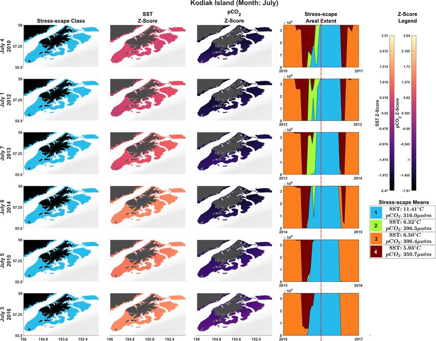
Blaisdell et al.                                                                                                                    Dynamic Stress-Scapes

                                            result shows that including growth rate data in stress-scape classification adjusts the
                                            training of the prSOM, enabling it to distinguish between regions where elevated sea
                                            surface temperature is negatively impacting growth rates. Classifications that rely solely
                                            on environmental data fail to distinguish these regions. With their incorporation of
                                            environmental and non-linear physiological variables across a wide spatio-temporal
                                            scale, stress-scapes show promise as an emerging methodology for evaluating the
                                            response of marine fisheries to changing ocean conditions in any dynamic marine
                                            system where sufficient data are available.
                                            Keywords: stress-scapes, Gulf of Alaska, machine learning, visualization, Pacific cod, multiple environmental
                                            stressors

INTRODUCTION                                                                      Ocean acidification is one such potential stressor and refers
                                                                                  to the gradual increase in hydrogen ions and consumption of
Environmental variability and associated trends induced by                        carbonate ions in marine systems in response to elevated levels
climate change can create unique and potentially stressful                        of anthropogenic carbon dioxide entering the ecosystem (e.g.,
conditions for marine fisheries that fluctuate through space                      Feely et al., 2004; Evans et al., 2014). The GOA, with the naturally
and time. Increasing water temperatures and ocean acidification                   lower concentrations of carbonate ions characteristic of high
related to changing ocean conditions have the potential to                        latitude marine habitats, is at higher risk for the effects of ocean
negatively impact individual fish – through direct and indirect                   acidification as additional losses of carbonate ions can lead to
effects – which can potentially impact fisheries by way of fishable               proportionally larger changes in seawater chemistry than would
biomass, annual stock productivity, and spatial shifts in the                     be expected in lower latitude systems (Fabry et al., 2009; Mathis
population outside of the traditional fishing areas (Holsman et al.,              et al., 2011). Additionally, the GOA and Kodiak Island regions are
2020; Laurel and Rogers, 2020). The Gulf of Alaska Pacific Cod                    known to have higher seasonal variability in natural surface pCO2
(Gadus macrocephalus) fishery is one example of a commercial                      levels (seasonal amplitudes of as much as 309.8 and 279.4 µatm,
fishery that is highly susceptible to changing ocean conditions.                  respectively) when compared to open ocean environments due
In recent years, Pacific Cod abundance has declined dramatically                  to upwelling conditions (Chen and Hu, 2019). Some interactions
in the Gulf of Alaska (GOA) ecosystem, leading to a fisheries                     between sea surface temperature and the carbonate system are
disaster declaration in 2018 and a closure of the federal fishery in              known – for example, carbon dioxide becomes less soluble in
2020 (Barbeaux et al., 2020). Quantifying the spatial and temporal                water as water temperature increases – but the full effects are not
footprint of modern environmental stressors on GOA Pacific Cod                    yet known in the context of physiological stress to living marine
is crucial for ensuring the accuracy of plans and forecasts for this              resources (Mathis et al., 2015).
valuable fishery.                                                                     Recent declines in Pacific Cod stocks are likely connected
    Decadal and long-term patterns influence the GOA’s thermal                    to changing thermal conditions in the GOA. Pacific Cod is a
variability due to warm-phase shifts of climatic phenomena and                    stenothermic species with peak hatch success occurring in 4–
background warming related to climate change. The GOA has                         5.5◦ C water (Laurel and Rogers, 2020) and optimal juvenile
also experienced two anomalous marine heatwave events in the                      growth occurring below 13◦ C in nursery habitats (Hurst et al.,
past decade. Between late 2013 and 2016, a marine heatwave                        2010). It is likely that Pacific Cod, like other stenothermic species,
occurred in the GOA that exceeded the magnitude and duration                      exhibit stage-specific responses to warming, with potential for
of any other heatwave on record in the region. This heatwave                      thermal bottlenecks between different life stages (Dahlke et al.,
event led to temperature anomalies greater than 2.5◦ C (Bond                      2020; Rogers et al., 2020). Early life stages may be particularly
et al., 2015; Di Lorenzo and Mantua, 2016) and unprecedented                      sensitive to changes in temperature due to higher metabolic rates
shifts in the region’s biological communities, including increases                in the embryonic, larval, and juvenile stages (e.g., Finn et al., 2002:
in harmful algal blooms, reductions in fishery recruitment, and                   Werner, 2002). Elevated temperatures in the GOA are associated
mass mortality of marine mammals and seabirds (Leising et al.,                    with high larval mortality of Pacific Cod (Doyle and Mier, 2016)
2015; Piatt et al., 2020; Suryan et al., 2021). In the summer of 2019,            and a larger size at nursery entry. During the 2014–2016 and the
the GOA was impacted by another marine heatwave, leading to                       2019 marine heatwaves, it is hypothesized that a loss of suitable
similarly extreme temperature anomalies (Amaya et al., 2020).                     spawning habitat during heatwave conditions contributed to
The increasing frequency and intensity of marine heatwaves in                     declines in Pacific Cod hatch success and consequent older life
the coming years are likely to coincide with challenges to marine                 stages (Laurel and Rogers, 2020).
fisheries’ long-term health (Oliver et al., 2018; Cornwall, 2019).                    Pacific Cod also appear to be moderately impacted by ocean
    In addition to thermal variability, there are several sources of              acidification in the GOA. Elevated levels of carbon dioxide in the
environmental variability that co-occur in the GOA and which                      water column during the first two weeks of the larval duration
have the potential to overlap, compound, or negate one another                    are associated with suppressed growth, although this trend has
in ways that are still not fully understood (Bopp et al., 2013).                  been shown to reverse as larvae grow (Hurst et al., 2019). By

Frontiers in Marine Science | www.frontiersin.org                             2                                         May 2021 | Volume 8 | Article 656088
Blaisdell et al.                                                                                                        Dynamic Stress-Scapes

the juvenile stage, effects of elevated carbon dioxide levels on         rely on data being identically distributed or independent (i.i.d).
growth largely disappear (Hurst et al., 2012). It is hypothesized        This feature is critical for classifying complex, potentially non-
that fishes are better able to withstand the effects of ocean            linear interactions like those found in data from spatio-temporal
acidification than calcifying marine invertebrates due to their          time series, which are not independent because the current year’s
high metabolism and ability to regulate their inter/intracellular        classification almost always depends on previous months, years,
acid-base balance (e.g., Melzner et al., 2009). However, elevated        and nearby regions.
levels of carbon dioxide could lead to several indirect impacts              Here, we introduce “stress-scapes” as a novel machine learning
on fishes including behavioral changes (e.g., Williams et al.,           framework to understand juvenile Pacific Cod’s response to
2019); changes in the biochemical structure of prey (e.g., Cripps        potential environmental stressors across the GOA ecosystem.
et al., 2016); and changes in the abundance of calcifying marine         Juvenile Pacific Cod was selected for this project due to
invertebrate prey (e.g., Lischka et al., 2011). Many of the direct       the availability of information and data related to the effects
and indirect impacts of ocean acidification on cod and other             of temperature and ocean acidification on early life stages.
marine finfish species are unknown, and the modest impacts               While there remain many unknown biological responses to
of ocean acidification observed in the laboratory may indeed             these stressors, both alone and in their potential interactive
be “significant” when compounded by other environmental                  effects, we incorporate the most recent available data on this
stressors or realized over longer time scales. Here, we do not           critical species for this proof-of-concept study. Stress-scapes
account for potential interaction between temperature and ocean          incorporate remotely sensed sea surface temperature (SST)
acidification as further studies are needed to better understand         data, pCO2 data, and estimated juvenile Pacific Cod specific
the interactive effects of these two variables on Pacific Cod            growth rate (SGR) into a prSOM algorithm to identify ocean
early life stages.                                                       conditions that may be stressful to juvenile Pacific Cod across
   Quantifying and visualizing environmental conditions in               a broad spatial and temporal scale. The juvenile Pacific Cod
space and time can be beneficial in understanding when and               stress-scape presented in this study is not intended as a
where the Pacific Cod fishery may be most influenced by                  comprehensive reconstruction of Pacific Cod growth history
changing ocean conditions in the GOA. By viewing the ocean               in response to environmental variability in the GOA, but
as a dynamic mosaic of physical and biogeochemical seascapes,            rather as a novel framework to visualize and classify potential
researchers, managers, and other end-users can efficiently               environmental stress on the species across space and time.
communicate information about environmental conditions in                In this way, the stress-scape framework is distinct from an
the ocean through space and time. This approach is known as              Individual-Based Model (IBM), which is a biophysical model that
dynamic seascape classification (Kavanaugh et al., 2014). Recent         describes fish growth, recruitment, and mortality as dependent
advances have allowed for the dynamic classification of ocean            on environmental factors (Hinckley et al., 1996; Hermann
regions based on multiple biophysical interactions observable            and Moore, 2009; Koenigstein et al., 2016). IBMs are often
by satellite remote sensing or marine ecosystem models (e.g.,            coupled with Regional Ocean Modeling Systems (ROMS) and
Kavanaugh et al., 2018). These dynamic classifications have              dispersal models to capture environmental conditions at depth
been used to predict biogeochemical processes (Kavanaugh                 and track the movement of fish in early life stages through
et al., 2014), phytoplankton structure and function (Kavanaugh           their environment (e.g., Stockhausen et al., 2019). An IBM for
et al., 2015; Montes et al., 2020), and individual species               Pacific Cod has already been developed for the GOA ecosystem
occurrences (Breece et al., 2016). The seascape ecology                  (Hinckley et al., 2019).
framework has potential utility for quantifying biological and               In our case study, we develop weekly stress-scapes from 2010
human responses to known environmental stressors, including              to 2016, including marine heatwave conditions in 2014–2016,
elevated temperature and ocean pCO2. By applying a dynamic               using existing juvenile Pacific Cod laboratory growth models
seascape framework in marine resource management contexts,               and remotely sensed environmental data. These stress-scapes
Klajbor (2020) established possible novel relationships between          are then evaluated spatiotemporally to determine how well they
dynamic ocean management principles and socioeconomic                    capture changing conditions both seasonally and interannually,
vulnerability in fishing communities.                                    including during the marine heatwave event. We then evaluate
   Large, biophysical time series like those used in a seascape          the sensitivity of the stress-scape model to the Pacific Cod
ecology approach have been classified in space and time                  SGR input variable to determine the importance of this variable
simultaneously using a probabilistic self-organizing map                 in influencing the model’s classification. Finally, we compare
(prSOM) machine learning algorithm (Kavanaugh et al., 2014,              the stress-scape model output to otolith-derived growth data
2016, 2018). The prSOM combines two statistical algorithms,              from juvenile Pacific Cod collected from Kodiak Island, AK to
K-Means and expectation-maximization, and a machine                      comment on the success of the model in capturing processes
learning algorithm called the Self-Organizing Map (Kohonen,              occurring in the field.
1990; Richardson et al., 2003) to approximate the multivariate
distribution of data as a mixture of Gaussians and uniform
distributions (Anouar et al., 1998; Lebbah et al., 2015). The            MATERIALS AND METHODS
prSOM algorithm has utility in capturing biological metrics,
such as Pacific Cod growth, in addition to environmental metrics         Environmental Data
because it is robust to non-linear relationships between variables       Sea surface temperature and sea-surface carbonate chemistry
and is topology-preserving. Also, the prSOM algorithm does not           data (pCO2 ) were collated for the GOA ecosystem between the

Frontiers in Marine Science | www.frontiersin.org                    3                                      May 2021 | Volume 8 | Article 656088
Blaisdell et al.                                                                                                          Dynamic Stress-Scapes

years 2010–2016 (see Supplementary Material: Appendix A for              The spatio-temporal z-scores were used to train the prSOM to
spatial extent of environmental data). Environmental data were           compute stress-scape classes across the GOA from 2010 to 2016
selected from publicly available modeled, in situ, and remotely          (Gregor et al., 2019); hence, the stress-scape classes represent
sensed products. The data’s temporal range was selected to               regions that similarly deviate from the spatio-temporal mean.
include dates before, during, and after the 2014–2016 marine
heatwave event. Sea surface temperature data were subset from            Juvenile Pacific Cod Growth Data
the National Oceanic and Atmospheric Administration (NOAA)               Juvenile Pacific Cod temperature-dependent growth data were
Optimum Reynolds Interpolation SST V2 product provided by                obtained from two existing experimental studies: Laurel et al.
the OAR/ESRL PSL, Boulder, Colorado, United States (Reynolds             (2016) and Hurst et al. (2010). These studies were all conducted
et al., 2002). The product is developed using a combination              in the laboratory using age-0 juveniles collected from the GOA
of in situ and remotely sensed data, producing weekly means              population. Similar growth data related to variable pCO2 are
on a one-degree grid. Associated variance related to each                currently unavailable for age-0 juvenile Pacific Cod [although see
point was also downloaded and used to calculate total error              Hurst et al. (2019) for earlier life stage responses]. As a proxy, we
related to the stress-scape classification. Sea-surface carbonate        used the pCO2 growth response of age-0 juvenile Walleye Pollock
chemistry data were subset from the NOAA National Center                 (Gadus chalcogrammus) based on experimental work from Hurst
for Environmental Information CSIR-ML6 v2019a Global Sea-                et al. (2012). While response to ocean acidification is variable
Surface pCO2 product. A smoothed mean monthly pCO2                       among marine finfish, Walleye Pollock are congeners of Pacific
product was selected from their ensemble mean product that is            Cod and share a similar growth response at the age-0 juvenile
calculated using a combination of 6 machine learning techniques.         stage (Laurel et al., 2016).
The smoothed product differs from their raw product, as a                   A weight-based growth model was used instead of a length-
3 × 3 × 3 convolution is applied to the data through time,               based growth model throughout this stress-scape analysis to
latitude, and longitude (Gregor et al., 2019). Mean monthly              better align with potential future bioenergetic applications of the
values ranged from 262.6 to 469.4 µatm in the study domain.              stress-scape to fish bioenergetics. Therefore, a specific growth rate
    Only the environmental data from the known spatial and               (SGR) model was used to approximate the percent change of fish
temporal ranges of Pacific Cod were included in the subsequent           wet weight over time. SGR were calculated from the formula:
machine learning training and stress-scape visualization,
                                                                                                 SGR = 100 eg − 1

ensuring that the selected data and resulting stress-scapes were
relevant to juvenile Pacific Cod distribution. Age-0 juvenile            where g is the instantaneous growth coefficient obtained from the
Pacific Cod are distributed in shallow, nearshore habitats,              equation:
typically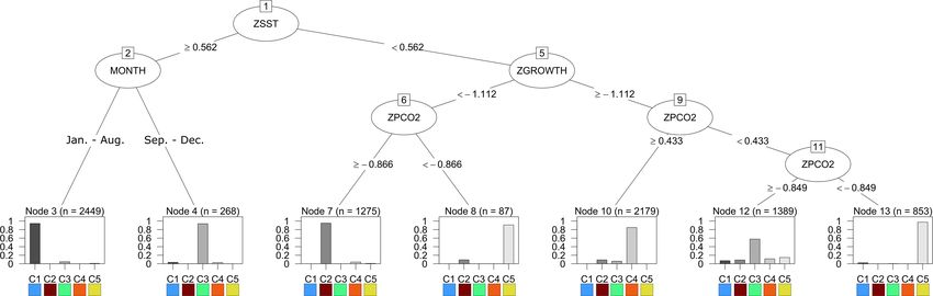
Blaisdell et al.                                                                                                            Dynamic Stress-Scapes

percent change in growth that would be expected under elevated             quality of each cluster and then reporting the average quality
pCO2 conditions. Growth under high pCO2 conditions was                     over all the clusters for increasing number of clusters. An optimal
represented by the equation:                                               number of clusters can be determined from the silhouette method
                                                                           by choosing a number K for which the quality of the clusters
             SGR = 0.061 + 0.297Temp − 0.013Temp2                          is greater than the quality of the K-1 and K + 1 clusters. The
                                                                           Gap Statistic works by computing the HAC algorithm for an
Classification of Stress-Scapes                                            increasing number of clusters. For each number of clusters, from
Stress-scapes were classified using remotely sensed observations           1 to 10, we computed the inter-cluster sum of square error, the
of SST; partial pressure of CO2 (pCO2 ) as an indicator of                 average quality of the clusters, and the gap statistic using the
the carbonate system; and the specific growth rate (SGR) of                clustGap() function in R.
juvenile Pacific Cod. The prSOM approximates the multivariate                 In order to evaluate the effects of anomalous heatwave
distribution of SST, pCO2 and SGR through space and time.                  conditions on the stress-scape classification results, classification
The prSOM was configured with 225 neurons in a 15 × 15                     results from 2010 to 2013 were compared to classifications during
neuron map. Previous efforts in the North Pacific found that               a known anomaly, the marine heatwave event of 2014–2016,
this configuration resulted in sufficiently large number of data           to more normal ocean conditions preceding the heatwave. In
points (e.g., >500) per node (Kavanaugh et al., 2014). The                 comparing the classification results, we identified a dominant
prSOM algorithm executed 50 epochs in order to give the prSOM              stress-scape and examined the qualities of the dominant stress-
enough time to converge. We applied Hierarchical Agglomerative             scape using a decision tree and a table to records the frequency
Clustering (HAC) to the 225 neurons grouping them into five                and the environmental characteristics of the stress-scapes.
individual stress-scapes (e.g., Saraceno et al., 2006; Hales et al.,       Further details describing our implementation of the prSOM are
2012; Kavanaugh et al., 2018).                                             provided in Supplementary Material: Appendix C.
    The SST, pCO2 , and SGR maps of the GOA were interpolated
using bilinear interpolation from 14 × 40 grid points to a                 Sensitivity Analysis
780 × 2340 image to classify stress-scape class boundaries in              We trained a second, bivariate prSOM to compare the results of
the remotely sensed data. The interpolated image was copied                the stress-scape to a classification that did not include juvenile
to the Graphics Processing Unit (GPU) memory and classified                Pacific Cod SGR. This bivariate classification allowed us to
according to the trained neurons’ weight vectors and variances             evaluate the sensitivity of the trivariate stress-scape framework
by identifying the stress-scape class most likely to generate              to the additional information gained by including the juvenile
each interpolated value in the GOA. Our unique prSOM                       Pacific Cod SGR variable in the training process. To account for
implementation classified the GOA in parallel using the GPU.               the reduced variance in the bivariate prSOM, we used the Gap
Parallel classification is an important distinction because many           Statistic to estimate 4 classes in the bivariate prSOM. We applied
visualization methods rely on processing done on the Central               Hierarchical Agglomerative clustering until the 225 neurons
Processing Unit (CPU), but the amount of data we needed                    were merged into 4 distinct stress-scape classes. We focused our
to classify made classification on the CPU impractical. Any                comparison efforts on the coastal regions near Kodiak Island.
consumer-grade GPU released in the past decade can classify
the entire GOA in a small number of clock cycles (∼1–100                   Pacific Cod Field Growth
clock cycles) by taking advantage of massively parallel processing.        Otolith structural analysis of juvenile Pacific Cod collected
In contrast, even with a parallel CPU implementation, the                  from Kodiak Island nurseries is being completed as part of a
number of clock cycles will range from 300,000 to 1.7 million              related study (Thalmann et al., unpublished data). Therefore,
clock cycles on most modern processors. There are 365 time                 after developing the lab-based model for juvenile Pacific Cod
slices, so the classification must be done 365 times; hence the            SGR, training the prSOM algorithm, and generating the mosaic
speedup is substantial.                                                    of stress-scapes across the coastal GOA, we estimated otolith-
    We selected 5 stress-scape classes from the HAC using the Gap          based SGR from these field-collected juveniles to compare with
Statistic (Tibshirani et al., 2001) which suggested 5 classes with 2       our stress-scape classifications of growth observed in nearshore
well separated classes and 3 less separated classes. Choosing an           Kodiak Island nursery habitat. This comparison aimed not to
optimal number of stress-scapes is difficult as there is no single         provide a comprehensive analysis of otolith data but rather to
metric that can select an ideal number of clusters with certainty,         identify a relationship between temporal patterns in the otolith-
and often, the statistically significant number of clusters does           based growth rates and temporal patterns in the stress-scapes.
not agree with domain expert analysis. For our implementation,             Juvenile Pacific Cod were collected in annual summer beach
we compared results from three different methods of clustering             seine surveys on Kodiak Island in 2010 and 2012–2016 through
evaluation: the elbow method, the silhouette method, and the               the NOAA Alaska Fisheries Science Center Fisheries Behavioral
Gap Statistic (see Supplementary Material: Appendix C). The                Ecology program. Samples were not available in 2011. Pacific Cod
elbow method works by estimating the amount of variance in the             were collected from two shallow (
Blaisdell et al. Dynamic Stress-Scapes
length, mm). Samples were then frozen (−20◦ C) and returned mm per day was examined for each year and compared to a mm/d
to Hatfield Marine Science Center in Newport, OR for post- laboratory growth model obtained from the same studies (Hurst
processing. During post-processing, standard length (mm) and et al., 2010; Laurel et al., 2016) as the laboratory SGR model used
wet weight (g) were measured, and otoliths were removed for in the stress-scape analysis.
analysis (Table 1). To estimate juvenile wet weight 8- and 16-d prior to capture,
Otolith structural analysis was used to generate growth we developed a second log-linear model with standard length
estimates for field-collected juveniles collected at Kodiak Island. and year as independent variables and wet weight as a dependent
Otoliths are calcium carbonate structures in the inner ear of variable (Multiple Linear Regression; R2 adj . = 0.96; P < 0.0001;
teleost fishes that can be used to determine age and growth of Supplementary Material: Appendix D). Wet weight from 8-
an individual (Pannella, 1971; Campana and Thorrold, 2001). and 16-d prior to capture was then determined using a second
Otolith size and body size are highly correlated in Pacific Cod proportional back-calculation model using estimated standard
(DiMaria et al., 2010; Miller et al., 2016), and daily formation length from 8- and 16-d prior to capture. Juvenile Pacific Cod
of otolith increments has been validated for Pacific Cod at 10◦ C SGR in the field was calculated in the same manner as the
up to 120 days post-hatch (Narimatsij et al., 2007). Sagittal laboratory SGR model described above from Hurst et al. (2010)
otoliths were mounted on glass slides using thermoplastic resin and Laurel et al. (2016). We utilized weight-based SGR calculated
and polished to expose the core in the transverse plane using from otoliths rather than length-based growth estimates for
Wetordry paper (800–2000 grit), Buehler lapping film (3–30 comparison to the stress-scape.
micron grit), and alumina slurry (0.3 micron). Polished otoliths To compare otolith-generated SGR estimates from the 8-
were imaged at 100× and 400× magnification using a Leica and 16- day periods prior to capture with the stress-scape, we
DM1000 compound microscope and a Levenhuk M1000 digital determined the dominant stress-scape class for coastal Kodiak
camera. Final otolith radius and otolith radius from 8 and 16 days Island at an 8-day resolution in July for each year between
prior to capture were quantified using increment analysis. Daily 2010 and 2016. Mean SGR from the dominant stress-scape
increments for these two 8-day growth periods (representing class was then compared to otolith-generated SGR for that year
three weeks of nursery residence at the same 8-day resolution using a paired t-test. Otolith-generated growth estimates for each
as the stress-scape model) were counted and measured using year were additionally compared to the temperature-dependent
ImagePro Premier software. Each otolith was interpreted three laboratory growth model using a paired t-test. We also compared
times with greater than 80% similarity in mean increment width otolith-derived growth rates in heatwave conditions in 2014–
between reads, and reads were averaged in order to compare 2016 to more normal conditions in 2010–2013 using a 1-way
otolith-generated estimates of growth to the stress-scape. analysis of variance.
First, we estimated fish length and mass at 8-d and 16-d
prior to capture based on otolith increment analysis, and then
estimated growth in length and mass over these two 8-d periods RESULTS
for comparison with the 8-d prSOM output. Otolith radius
measurements and fish standard length were log-transformed Stress-Scape Analysis
to meet parametric assumptions, and a log-linear model with Utilizing the prSOM and HAC, we resolved 5 unique stress-
otolith radius, year, and their interaction as independent scapes across the GOA that quantified the spatio-temporal
variables and standard length as a dependent variable was footprint of changing ocean conditions and the modeled specific
developed (Multiple Linear Regression; R2 adj . = 0.85; P < 0.0001; growth rate (SGR) of juvenile Pacific Cod. Table 2 describes
Supplementary Material: Appendix D). Using this relationship, the means and standard deviations for the SST, pCO2 , and
we developed a proportional back-calculation model to estimate SGR values of each of the resolved classes. Stress-scape classes
fish size 8- and 16-d prior to capture using the measured otolith were determined and distinguished semantically through a
radius from 8- and 16-d prior to capture (Francis, 1990; Campana decision-tree of z-scores for each input variable, including the
and Jones, 1992). Length-based growth of juvenile Pacific Cod in characteristics of each decision mode, which effectively describes
TABLE 1 | Annual sample sizes, average fish size, mean July ocean temperature, mean July pCO2 levels, and ocean conditions for juvenile Pacific Cod captured
annually in July 2010 and 2012–2016 from Kodiak Island, AK.
Year Sample size (n) Fish size (SL; mm) July temperature (◦ C) July pCO2 (µatm) Ocean conditions
2010 23 43.35 ± 0.82 10.07 ± 0.15 288.31 Normal
2012 17 41.47 ± 1.17 10.04 ± 0.32 291.00 Normal
2013 19 50.00 ± 1.43 11.64 ± 0.40 295.02 Normal
2014 19 51.79 ± 1.53 12.52 ± 0.23 287.90 Heatwave
2015 9 47.67 ± 1.29 11.69 ± 0.21 300.08 Heatwave
2016 20 62.40 ± 1.16 12.85 ± 0.25 313.57 Heatwave
Samples were not collected in 2011. All samples were collected through the NOAA Alaska Fisheries Science Center (AFSC) as part of the Fisheries Behavioral
Ecology Program.
Frontiers in Marine Science | www.frontiersin.org 6 May 2021 | Volume 8 | Article 656088Blaisdell et al. Dynamic Stress-Scapes
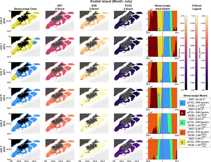
TABLE 2 | Mean values for each of the 5 resolved stress-scapes. for the sensitivity analysis. By excluding the SGR variable, the
dominant stress-scape for coastal Kodiak Island was reclassified
SST (◦ C) SGR % WW
Day pCO2 (µatm) Count Color
to a new stress-scape class 1 (blue), which identifies a mean
Mean Std Mean Std Mean Std SST of 10.42 ± 2.48◦ C and mean pCO2 concentration of
359.4 ± 33.66 µatm across all years of analysis. Stress-scape
Class 1 10.42 2.48 1.4 0.16 359.4 33.66 2895 class 1 of the bivariate model corresponds to stress-scape class
Class 2 6.25 2.38 1.04 0.28 340.3 39.99 1856 3 of the trivariate-model. Figure 4 shows the dominant yearly
Class 3 9.34 2.62 1.34 0.19 346.9 37.12 1515 classes for the bivariate prSOM sensitivity analysis near coastal
Class 4 6.36 2.14 1.06 0.24 370.4 38.18 2403 Kodiak Island during the first week of July 2010 and 2012–
Class 5 7.85 2.25 1.22 0.23 339.1 36.41 1331 2016 and should be evaluated using Table 3. Stress-scape class
Means and standard deviations are included for SST, SGR measured in percent wet 1 is distinguished from the other three classes with its higher-
weight per day (%WW/day), and pCO2 concentration values along with a count than-average SST and near average pCO2 concentrations. The
of the number of remotely sensed data points belonging to each class and their
corresponding classification color. The stress-scapes were classified based on the
bivariate prSOM groups the two higher temperature classes of
provided environmental data and the decision tree outlined in Figure 1. the trivariate dynamic stress-scape together because it lacks the
SGR variable necessary for distinguishing between these classes.
In addition, the bivariate prSOM is unable to distinguish between
how the classes were sorted (Figure 1). Stress-scape classes 2, 3, heatwave conditions and more normal ocean conditions in the
4, and 5 (maroon, green, orange, and yellow) were distinguished GOA, with stress-scape class 1 dominant across all six years
by their respective growth rate input variables when they were of the analysis.
decided by node 5. This highlights the non-linear relationship
between SST and SGR. Class 1 (blue) was primarily distinguished Juvenile Nursery Growth
by differences in SST and pCO2 .
The dynamic stress-scape underestimated the observed juvenile
The stress-scape analysis identified distinct classes that
Pacific Cod SGR in its classification schema for coastal Kodiak
corresponded to heatwave conditions in 2014–2016 compared
Island by 39–187% across all six years of the analysis (Figure 5).
to more normal ocean conditions in 2010–2013 for both
Mean July SGR from the dominant stress-scape for coastal
coastal Kodiak Island (Figure 2) and the larger GOA coastal
Kodiak Island differed significantly from otolith-derived SGR
ecosystem (Figure 3). Animated versions of these figures with
for both the last 8 days of growth and the penultimate 8 days
corresponding ribbon plots that show how the stress-scapes shift
of growth (paired t-test; last 8 days: t5 = 6.72; P = 0.0011;
and progress through time can be found in Supplementary
penultimate 8 days: t5 = 6.94; P = 0.0009). Otolith-derived
Material: Appendix E, Supplementary Videos 1, 2. At both the
SGR were between 10 and 105% higher than the laboratory
Kodiak and regional scales, seasonal and interannual patterns
growth model across all six years for both the last 8 days of
emerge in the incidence of each of the classes. Classes 2 and 5
growth and the penultimate 8 days of growth (paired t-test; last
contract over time, supplanted by expansions (in space and time)
8 days: t5 = 4.69; P = 0.0053; penultimate 8 days: t5 = 5.39;
of classes 1 and 4. Class 2 is the low SST class that seems to be
P = 0.0029). In contrast, otolith-derived mm/d growth were
replaced by high pCO2 in class 4. Class 5, the pre-heatwave late
between 13% and 79% lower than the laboratory growth model
spring-early summer class, is replaced by class 3, characterized by
for both the last 8 days of growth and the penultimate 8 days
high SST, during heatwave years. Class 3 starts appearing earlier
of growth (paired t-test; last 8 days: t5 = 6.54; P = 0.0012;
and persisting each year during the heatwave.
penultimate 8 days: t5 = 5.71; P = 0.0023). Across all years,
In July, stress-scape class 5 (yellow) dominated the areas
field estimated growth rates were similar between heatwave
around Kodiak Island in 2010 and 2012, whereas stress-scape
conditions in 2014–2016 compared to more normal ocean
class 3 (green) expands both around Kodiak and within the
conditions in 2010–2013 (1-way ANOVA; F1 ,102 = 0.75; P = 0.39),
greater GOA area during heatwave conditions in 2014, 2015,
highlighting the difference in potential SGR predicted by the
and 2016. In 2013, stress-scape class 3 and stress-scape class
prSOM and the realized SGR observed in the field during
5 were both present throughout the coastal GOA. Stress-
heatwave conditions.
scape class 3 was characterized by above average temperatures
(10.42 ± 2.48◦ C), higher pCO2 , concentrations (359.4 ± 33.66
µatm), and high juvenile Pacific Cod SGR (1.40 ± 0.16% Wet
DISCUSSION
weight/day). In contrast, stress-scape class 5 was characterized
by near average temperatures (7.85 ± 2.25◦ C), lower pCO2 The application of seascape ecology methods to the evaluation
concentrations (339.1 ± 36.41 µatm), and near average SGR of potential environmental stressors across a wide spatio-
(1.22 ± 0.23% Wet weight/day). temporal scale on juvenile GOA Pacific Cod represents a
new approach to visualize and synthesize the effects of
Sensitivity Analysis extreme environmental variability on marine fisheries. Five
The bivariate prSOM, trained on SST and pCO2 but excluding dynamic stress-scapes were resolved from 2010 to 2016 that
SGR, resolved four stress-scape classes for the coastal GOA. correspond to unique environmental conditions and growth
Table 3 describes the means and standard deviations for the responses of juvenile Pacific Cod. Stress-scape identity and
SST and pCO2 values of each of the resolved classes used spatial extent changed as a function of time, capturing unique
Frontiers in Marine Science | www.frontiersin.org 7 May 2021 | Volume 8 | Article 656088Blaisdell et al. Dynamic Stress-Scapes FIGURE 1 | The results of the decision tree trained on the output of stress-scape classification using 5-stress-scapes and 4 variables: SST z-score (ZSST), juvenile Pacific Cod SGR z-score (ZGROWTH) measured in percent wet weight per day (%WW/day), pCO2 concentration (µatm) z-score (ZPCO2), and the month of the remotely sensed observation (MONTH). Each node of the decision tree represents a decision about the variable labeling the vertex and is labeled with a number. The root node represents a decision about the monthly z-score of SST. If the pixel’s SST is greater than.562 standard deviations above the mean SST value across the entire GOA from 2010 to 2016, the left branch is taken; otherwise, the right branch is taken. Note that by including SGR (ZGROWTH) as a classification variable we can make biologically relevant interpretations of the stress-scape classes that are classified by the right branch of node 1. The bar graph provides the percent of each class that is classified by each leaf node of the tree. FIGURE 2 | Dominant yearly stress-scape classes for coastal Kodiak Island during the first week of July 2010 and 2012–2016. Heatwave conditions are present in 2014–2016. Column 1 highlights the dominant stress-scape classes for coastal Kodiak Island. Column 2 is the z-score for SST; Column 3 is the z-score for SGR, and Column 4 is the z-score for pCO2 . The red line marks the time shown in the figure across all years. Dark purple z-scores are below average and yellow z-scores are above average for that variable. An animated version of this figure can be found in Supplementary Material: Appendix E and Supplementary Video 1. conditions and responses during the 2014–2016 marine heatwave during heatwave years that did not dominate prior to heatwave compared to the previous cooler conditions. Stress-scapes years. This dominant stress-scape corresponds to observed captured non-linear biological responses to the environment: elevated growth rates from the otolith data from Kodiak when SGR was included as a variable (in addition to SST Island. Even though SGR is a function of SST, including fish and pCO2 ) there was a single stress-scape that dominated growth as a variable in the stress-scape captures patterns of Frontiers in Marine Science | www.frontiersin.org 8 May 2021 | Volume 8 | Article 656088
Blaisdell et al. Dynamic Stress-Scapes
FIGURE 3 | Ribbon plot showing total Stress-scape class area per time slice. Each column represents a single slice through time of the entire GOA. A stress-scape
dominates in time if it persists along the x-axis. For example, in 2016, stress-scape class 1 was spatiotemporally dominant. From 2014 to 2016 stress-scape classes
1 and 4 dominate for a longer period than in 2010–2013. Classes 1 and 4 are coincident with the anomalous elevated growth rates seen in the otoliths data.
A seasonal and interannual pattern emerges in the incidence of each of the classes: The spatiotemporal footprint of classes 2 and 5 contract over time, supplanted
and are replaced by expansions of classes 1 and 4. Class 2, a low SST class, that seems to be replaced by high pCO2 class 4. Class 5, the pre-heatwave summer
class, is replaced by the high SST class 3, which starts appearing earlier and persisting each year during the heatwave. This ribbon plot can be viewed as a video
alongside a map of the GOA in Supplementary Material: Appendix E and Supplementary Videos 1, 2.
growth that are comparable to those derived from otoliths GOA during marine heatwave conditions. Pacific Cod, like
in situ. many stenothermic fish species, are likely to experience life
Output from the stress-scape visualization indicated that stage-specific thermal bottlenecks, especially in the embryonic
juvenile Pacific Cod experienced moderately higher potential and adult spawner stages where the fish may be particularly
growth during heatwave years compared to more normal vulnerable to environmental variability (Dahlke et al., 2020).
environmental conditions. Accelerated growth is a common It has been shown that Pacific Cod hatch success is strongly
bioenergetic response of teleost fishes to warmer ocean correlated with temperature, with hatch success most optimal
conditions, with increased temperatures contributing to at temperatures between 3 and 6◦ C (Laurel and Rogers, 2020).
increased metabolism and faster growth as long as caloric and During the 2014–2016 marine heatwave, optimal spawning
oxygen requirements are adequately met, until an upper limit habitat was restricted to shallower regions and earlier times
above which growth will begin to decline (e.g., Beauchamp, of the year, and this decline in suitable spawning habitat may
2009; Thalmann et al., 2020). These results suggest that warmer have led to widespread reductions in reproductive output.
temperatures during the juvenile life stage led to faster growth Those individuals that survived the thermal bottleneck at the
than would be expected during normal ocean conditions. embryonic life stage may have experienced higher growth rates
However, in contrast with these observed potential growth during the larval and juvenile life stages in warmer conditions,
rates, Pacific Cod abundance was anomalously low in the especially if prey was available and “matched” in time and space
(Laurel et al., 2021). Additionally, juvenile Pacific Cod collected
in Kodiak nurseries were two to four months old by July and
the product of selective mortality. In poor survival years, such
TABLE 3 | Mean values for each of the 4 resolved stress-scapes that were as 2015, slower growing or smaller fish can experience higher
classified to test the significance of the growth rate variable.
rates of mortality, leaving only the faster growing fish in the
SST (◦ C) pCO2 (µatm) Count Color population (Litvak and Leggett, 1992; Sogard, 1997). Thus, the
results from the stress-scape visualization likely do not capture
Mean Std Mean Std the full impact of the 2014–2016 marine heatwave on Pacific
Cod simply because it captures only a snapshot of the entire
Class 1 11.41 1.84 316.0 19.02 3836
Pacific Cod life history, but the approach highlights the spatial
Class 2 6.32 1.34 296.3 16.79 557
and temporal extent of anomalous and potentially stressful
Class 3 6.50 1.96 396.4 17.25 3939
conditions. With the addition of information on prey quantity
Class 4 5.93 1.93 350.7 16.79 1668
and quality and pCO2 and temperature data throughout the
Means and standard deviations are included for SST and pCO2 concentrations as water column, a more comprehensive exploration of the effects
well as the number of remotely sensed data belonging to each class (count) and
corresponding classification color for each of the 4 resolved classes for the bivariate
of the heatwave throughout the life history of Pacific Cod, and
prSOM sensitivity analysis. potentially other species, would be possible.
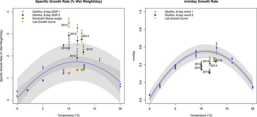
Frontiers in Marine Science | www.frontiersin.org 9 May 2021 | Volume 8 | Article 656088Blaisdell et al. Dynamic Stress-Scapes FIGURE 4 | Dominant yearly classes for the bivariate prSOM sensitivity analysis near coastal Kodiak Island during the first week of July 2010 and 2012–2016. Normal ocean conditions are present in 2010–2013, and heatwave conditions are present in 2014–2016. Column 1 highlights the dominant stress-scape classes for coastal Kodiak Island. Column 2 is the z-score for SST, and Column 3 is the z-score for pCO2 . The final column gives the areal extent of each stress-scape class. The red line indicates the time slice of the areal extent (see Supplementary Material: Appendix E and Supplementary Videos 1, 2). FIGURE 5 | Comparison of juvenile Pacific Cod SGR (left panel;% wet weight/day) and mm/day growth rate (right panel) from individuals collected from Kodiak Island, AK in July 2010 and 2012–2016. Final 8 days of otolith growth prior to capture are represented by dark green triangles, and penultimate 8 days of otolith growth are represented by light green triangles. Laboratory models are represented by the blue growth curve and blue circles. Specific growth rate from the dominant stress-scapes in July near Kodiak Island are represented by gold diamonds. Error bars represent standard error. Gray polygons represent confidence and prediction intervals of the laboratory growth model. Frontiers in Marine Science | www.frontiersin.org 10 May 2021 | Volume 8 | Article 656088
Blaisdell et al.                                                                                                            Dynamic Stress-Scapes

    Otolith-derived SGR rates for field-collected juvenile Pacific          the effects of ocean acidification in the presence of elevated
Cod were between 39 and 187% higher than those predicted by                 water temperatures due to a heightened stress response (Harvey
the dominant stress-scape class for coastal Kodiak Island across            et al., 2013; Kroeker et al., 2013, 2014). However, fishes tend to
most years of the analysis. This pattern highlights a potential             be less sensitive than marine invertebrates to increased carbon
underestimation of the stress-scape machine learning algorithm              dioxide in the water column even in the face of elevated
in predicting juvenile Pacific Cod growth in the field. The most            temperature conditions due to their increased metabolism (e.g.,
parsimonious explanation for this result is that the temperature            Enzor et al., 2017), highly developed acid/base regulatory systems
data used in the model did not accurately reflect shallow nursery           (e.g., Melzner et al., 2009), and potential for energy reallocation
conditions that often exceed 15◦ C in summer around Kodiak                  (e.g., Laubenstein et al., 2018). Studies examining the effects
Island (Laurel et al., 2012). However, the laboratory model for             of elevated carbon dioxide concentrations on the early life
SGR underestimated otolith-derived SGR across most years,                   stages of Alaskan gadids (including Walleye Pollock, a congener
while the laboratory model for mm/d growth overestimated                    of Pacific Cod that shares a similar growth response at the
otolith-derived growth. Growth in mass and growth in length                 juvenile stage), show limited impacts to growth response (Hurst
are related but can reflect differences in energy allocation. For           et al., 2012, 2019). Therefore, we expect interactive effects of
example, there is some evidence that seasonality can influence              temperature and ocean acidification on SGR are likely minimal
fish growth in the field, with fish adding more length earlier              for juvenile Pacific Cod.
in the season when conditions are favorable for feeding, and                   While previous dynamic classifications of the ocean include
then adding more mass later in the season to better prepare                 lower trophic level responses to environmental forcing (e.g., chl-
for winter conditions (e.g., Hurst and Conover, 2003; Hurst,                a or carbon; Kavanaugh et al., 2014, 2018), the incorporation
2007). Field growth may also exceed laboratory-based growth                 of fish physiology represents a notable revision and test of
models due to a number of in situ processes, including higher               non-linear responses of higher trophic levels. Furthermore,
food quality in the field (e.g., Mazur et al., 2007), favorable             our sensitivity analyses suggests that exclusion of biological
conditions in nearshore nursery habitat (e.g., Beck et al., 2001;           responses results in an overly simple classification model. The
Hinckley et al., 2019), and the effects of seasonality on growth            bivariate prSOM (without growth rate) exhibited fewer output
rates, with juveniles feeding more vigorously in summer months              stress-scape classes compared to the full model and grouped
to prepare for winter (e.g., Schwalme and Chouinard, 1999).                 several output classes together. In addition, the bivariate prSOM
In 2014, 2015, and 2012, two heatwave influenced years and                  was unable to distinguish between heatwave conditions in
a cool ocean year, respectively, juvenile Pacific Cod exhibited             2014–2016 and more normal conditions in 2010–2013, with
SGR in the field that were modestly higher than predicted from              the dominant class remaining the same across all six years.
the laboratory temperature-dependent growth rate model. We                  Due to the quadratic relationship of Pacific Cod growth to
note that the 2012 cohort of Pacific Cod was the strongest on               ocean temperature (Hurst et al., 2010; Laurel et al., 2016),
record in the GOA since 1977, and growth was likely elevated in             output classes in the full dynamic stress-scape model were
response to particularly favorable ocean conditions in that year            able to successfully distinguish between similar growth rates
and the production of multiple cohorts of juveniles (Hinckley               that occurred in response to two different temperature ranges
et al., 2019). In the unfavorable ocean conditions occurring                by classifying them into two separate output classes (classes 1
during the marine heatwave event in 2014 and 2015, only                     & 2). By including the biologically relevant growth response
the fastest growing individuals were likely to survive to the               into the stress-scape, we could distinguish temperatures that
juvenile life history stage, inflating the observed growth response         were high enough to negatively impact growth rate from
of the survivors (e.g., Ricker, 1969; Litvak and Leggett, 1992;             temperatures that were conducive to ideal growth. The utility of
Moss et al., 2005). The variability between observed growth                 dynamic stress-scapes in capturing non-linear growth patterns
rates in the field and classified growth rates in the stress-scape          could be expanded to include more complex biological patterns
suggests that future iterations of the stress-scape may benefit             as indicators of changing ocean conditions, such as those
from added parameters related to selective mortality, foraging              associated with prey quality and quantity (e.g., Daly et al., 2017),
conditions, and additional environmental parameters related to              predation (e.g., Fennie et al., 2020), or metabolic rate (e.g.,
ocean conditions.                                                           Chung et al., 2019).
    In this analysis, we assume that the effects of temperature and            Machine learning models show promise in classifying marine
pCO2 on Pacific Cod growth are additive. We do not account                  heatwave events because they can generalize to regions of the
for potential interaction between these two environmental                   ocean where there is limited data by being trained on more
variables as further studies are needed to elucidate the interactive        data-rich regions with similar conditions and then using the
effects between warming and ocean acidification on the growth               model to detect heatwave conditions. While there are several
of Pacific Cod early life stages. We acknowledge that the                   recent, well-received approaches to classifying marine heatwave
potential for interactive effects between temperature and pCO2              events (e.g., Hobday et al., 2016, 2018; Oliver et al., 2018),
on juvenile Pacific Cod growth may increase uncertainty in                  many of these approaches exclude biological response in their
stress-scape classification and contribute to the deviation between         classification schema for marine heatwaves. Our dynamic
Pacific Cod growth observed in the field compared to growth                 stress-scape classification of the GOA, which uses sea-surface
classified by the stress-scape. In general, early life stages of            measurements, successfully distinguished between marine
marine organisms tend to exhibit an increased sensitivity to                heatwave conditions in 2014–2016 and more historically normal

Frontiers in Marine Science | www.frontiersin.org                      11                                       May 2021 | Volume 8 | Article 656088
Blaisdell et al. Dynamic Stress-Scapes
ocean conditions in 2010–2013. In general, stress-scape classes is used at each iteration, but the distribution is uniform. The
that corresponded to heatwave conditions exhibited higher IBM/ROMS models could be used to estimate the probability
SST, moderate pCO2 concentrations, and elevated juvenile of a juvenile Pacific Cod encountering potentially stressful
Pacific Cod SGR. Stress-scapes that corresponded to more conditions at each ocean pixel. This distribution could be
normal ocean conditions exhibited moderate SST, lower pCO2 used to inform the sampling method at each epoch of the
concentrations, and moderate SGR. Dynamic stress-scapes prSOM so that the training data is more likely to represent
effectively present the biological footprint of remotely sensed the environmental context of the juvenile Pacific Cod. Our
oceanographic data by characterizing spatio-temporal changes stress-scape framework is not intended as a substitute for an
in the modeled SGR of juvenile Pacific Cod. The stress-scape IBM, and it does not offer a comprehensive reconstruction
framework shows promise in for merging spatio-temporal data of juvenile Pacific Cod growth history in the GOA (but see
and biological models to understand how heatwave conditions Hinckley et al. (2019) for an IBM currently in place for GOA
across a wide spatial and temporal range might affect living Pacific Cod). Rather, the stress-scape represents a new way to
marine resources. visualize changes in both environmental conditions and Pacific
Our methods are not without limitations. The prSOM Cod growing conditions before and during a marine heatwave
algorithm was chosen for this analysis because its topology event. Pacific Cod otoliths are used in the context of this study
preserving nature and its sensitivity to non-linear data. to support and serve as a point of comparison to the stress-
However, the prSOM implementation does not use k-fold scape classification of SST, pCO2 , and laboratory-derived juvenile
cross validation to avoid overfitting, which would improve the Pacific Cod SGR.
classification results. Future efforts would include t-distributed In summary, stress-scapes offer three new and novel features
stochastic neighbor embedding (t-SNE; Maatan and Hinton, relevant to the fields of marine resource management, ocean
2008), which provides a well-defined “optimal solution,” ecology and fisheries science. First, stress-scapes are based
lends itself to visualization of higher dimensional data (e.g., on both remotely sensed data and models that approximate
>3) and thus inclusion of additional in juvenile Pacific biological response to remotely sensed environmental data.
Cod fitness variables. Additionally, HAC can have issues Second, machine learning models can generalize to regions of
when the geometry of the data is not flat (as is the case ocean where there is limited data by being trained on data
with the relationship between sea-surface temperature and that share similar conditions. Third, stress-scapes use machine
growth rate). The DBSCAN (Ester et al., 1996) and OPTICS learning algorithms that train on spatially relevant data, in this
(Ankerst et al., 1999) algorithms could replace Hierarchical case based on temperature-growth models to approximate the
Agglomerative Clustering and be used in conjunction with growth rate of juvenile Pacific Cod. This produces an output
a prSOM or t-SNE machine learning algorithm to provide that is potentially relevant for management in multiple fields
a better stress-scape classification that distinguishes regions and at multiple spatial and temporal scales. Environmentally, the
where the temperature is warm enough to constrain growth stress-scapes are useful metrics that can benefit ecosystem-based
from regions where the temperature is conducive to optimal and dynamic approaches to management of marine resources
growth. Our visual results are a preliminary effort to introduce (Kavanaugh et al., 2016). From a management perspective, the
a visual system. In future work we will consider incorporating biological relevance of the stress-scapes can be used to trace or
immersive visualization techniques for visual exploration even forecast potentially stressful conditions for a focus species.
of the ocean and coordinated multi-view visualization on Downstream effects on socioeconomic conditions of resource
the different types and sources of data for decision making. users could also be identified by aligning the occurrence and
Efforts to expand on visualization within the fisheries longevity of stress-scape classes in space and time with economic
community suggest interest in developing fast, scalable and indicators and extraction data. The process is extremely flexible
explorative tools for fisheries scientists to understand the and can handle large amounts of many types of time series data,
relationship between ocean variables, marine resources, and furthering its utility.
the algorithms used to process data from these two domains
(Hermann and Moore, 2009).
Finally, our temperature-dependent growth model does not DATA AVAILABILITY STATEMENT
incorporate factors like prey quality, prey quantity, ocean
currents, or ocean conditions at depth. Individual Based The raw data supporting the conclusions of this article will be
Modeling (IBM) and Regional Ocean Modeling Systems (ROMS) made available by the authors, without undue reservation.
incorporate many of these factors and can be used to generate
a spatial footprint of fish dispersal (Stockhausen et al., 2019).
Information on the dominant dispersal pathways of Pacific Cod ETHICS STATEMENT
early life stages from an IBM/ROMS model could be paired
with the stress-scapes by developing the duration of residence Ethical review and approval was not required for the animal
in each stress-scape. On a related note, IBM/ROMS models study because the field work was conducted solely by NOAA’s
could be used to improve the data sampling used to train the Alaska Fisheries Science Center Laboratory in Newport, Oregon.
prSOM. Currently, remotely sensed data are sampled uniformly Animal tissue, in this case otoliths, was provided to OSU several
at random at each epoch, where a different random sample years after collection. This research was carried out in accordance
Frontiers in Marine Science | www.frontiersin.org 12 May 2021 | Volume 8 | Article 656088You can also read