Diapycnal mixing across the photic zone of the NE Atlantic
←
→
Page content transcription
If your browser does not render page correctly, please read the page content below
Ocean Sci., 17, 301–318, 2021
https://doi.org/10.5194/os-17-301-2021
© Author(s) 2021. This work is distributed under
the Creative Commons Attribution 4.0 License.

Diapycnal mixing across the photic zone of the NE Atlantic
Hans van Haren, Corina P. D. Brussaard, Loes J. A. Gerringa, Mathijs H. van Manen, Rob Middag, and
Ruud Groenewegen
Royal Netherlands Institute for Sea Research (NIOZ), P.O. Box 59, 1790 AB Den Burg, the Netherlands

Correspondence: Hans van Haren (hans.van.haren@nioz.nl)

Received: 17 July 2020 – Discussion started: 3 August 2020
Revised: 8 January 2021 – Accepted: 12 January 2021 – Published: 17 February 2021

Abstract. Variable physical conditions such as vertical tur-      1   Introduction
bulent exchange, internal wave, and mesoscale eddy action
affect the availability of light and nutrients for phytoplank-    The physical environment is important for ocean life, includ-
ton (unicellular algae) growth. It is hypothesized that changes   ing variations therein. For example, the sun stores heat in
in ocean temperature may affect ocean vertical density strat-     the ocean with a stable vertical density stratification as re-
ification, which may hamper vertical exchange. In order           sult. Generally, stratification hampers vertical turbulent ex-
to quantify variations in physical conditions in the north-       change because of the required work against (reduced) grav-
east Atlantic Ocean, we sampled a latitudinal transect along      ity before turbulence can take effect. It thus hampers a sup-
17 ± 5◦ W between 30 and 63◦ N in summer. A shipborne             ply of nutrients via a turbulent flux from deeper waters to the
conductivity–temperature–depth (CTD) instrumented pack-           photic zone. However, stratification supports internal waves,
age was used with a custom-made modification of the pump          which (i) may move near-floating particles like phytoplank-
inlet to minimize detrimental effects of ship motions on its      ton (unicellular algae) up and down towards and away from
data. Thorpe-scale analysis was used to establish turbulence      the surface and (ii) may induce enhanced turbulence via ver-
values for the upper 500 m from three to six profiles ob-         tical current differences (shear) resulting in internal waves
tained in a short CTD yo-yo, 3 to 5 h after local sunrise.        breaking (Denman and Gargett, 1983). Such changes in the
From south to north, average temperature decreased together       physical environment are expected to affect the availability
with stratification while turbulence values weakly increased      of phytoplankton growth factors such as light and nutrients.
or remained constant. Vertical turbulent nutrient fluxes did         Climate models predict that global warming will reduce
not vary significantly with stratification and latitude. This     vertical mixing in the oceans (e.g. Sarmiento et al., 2004).
apparent lack of correspondence between turbulent mixing          Mathematical models on system stability suggest that re-
and temperature is likely due to internal waves breaking (in-     duced mixing may generate chaos behaviour in phytoplank-
creased stratification can support more internal waves), act-     ton production, thereby enhancing variability in carbon ex-
ing as a potential feedback mechanism. As this feedback           port into the ocean interior (Huisman et al., 2006). However,
mechanism mediates potential physical environment changes         none of these models include potential feedback systems like
in temperature, global surface ocean warming may not affect       internal wave action or mesoscale eddy activity. From obser-
the vertical nutrient fluxes to a large degree. We urge mod-      vations in the relatively shallow North Sea it is known that
ellers to test this deduction as it could imply that the future   the strong seasonal temperature stratification is marginally
summer phytoplankton productivity in stratified oligotrophic      stable, as it supports internal waves and shear to such extent
waters would experience little alterations in nutrient input      that sufficient nutrients are replenished from below to sustain
from deeper waters.                                               the late-summer phytoplankton bloom in the euphotic zone
                                                                  that became depleted of nutrients after the spring bloom (van
                                                                  Haren et al., 1999). This challenges the current paradigm in
                                                                  climate models.

Published by Copernicus Publications on behalf of the European Geosciences Union.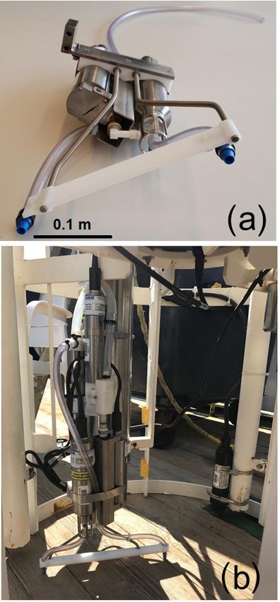
302                                         H. van Haren et al.: Diapycnal mixing across the photic zone of the NE Atlantic

   In this paper, the objective is to resolve the effect of ver-
tical stratification and turbulent mixing on nutrient supply to
the euphotic zone of the open ocean. For this purpose, up-
per 500 m ocean shipborne conductivity–temperature–depth
(CTD) observations were made in association with those on
dissolved inorganic nutrients during a survey along a tran-
sect in the NE Atlantic Ocean from midlatitudes (30◦ ) to
high (63◦ ) latitudes in summer. Throughout the survey, me-
teorological and sea-state conditions were favourable for ad-
equate sampling and wind speeds varied little between 5 and
10 m s−1 , independent of locations. All CTD observations
were made far from lateral, continental boundaries and at
least 1000 m vertically away from bottom topography (i.e.
far from internal-tide sources). The NE Atlantic is charac-
terized by abundant (sub-)mesoscale eddies especially in the
upper ocean (Charria et al., 2017) that influence local plank-
ton communities (Hernández-Hernández et al., 2020). The
area also shows continuous abundant internal wave activity
away from topographic sources and sinks, with the semidi-
urnal tide as a main source from below and atmospherically
induced inertial motions from above (e.g. van Haren, 2005,
2007). However, the sampled upper 500 m zone transect is
not known to demonstrate outstanding internal wave source
variations. Previous observations (van Haren, 2005) and Hi-
biya et al. (2007) have shown that a diurnal critical latitude
                                                                    Figure 1. Bathymetry map of the northeast Atlantic Ocean based
enhancement of near-inertial internal waves due to subhar-          on the 9.1 ETOPO-1 version of satellite altimetry-derived data by
monic instability only occurs sharply between 25 and 30◦ N.         Smith and Sandwell (1997). The numbered circles indicate the CTD
The present observations are all made poleward of this range.       stations, at station 17 (x) no turbulence parameter and only nutri-
Likewise, the Henyey et al. (1986) model on latitudinal vari-       ent sampling were done. At stations 1 and 2 no DFe samples were
ation in internal wave energy and turbulent mixing (Gregg           taken; at station 18 no nutrient samples were taken. Depth contours
et al., 2003) predicts changes by a maximum factor of 1.8 be-       are at 2500 and 5000 m.
tween 30 and 63◦ , but this value is relatively small compared
with errors, typically a factor of 2 to 3, in turbulence dissi-
pation rate observations. Likewise, from the equal summer-          to north. The present observations go deeper to 500 m, also
time meteorological conditions little variation is expected in      across the non-seasonal more permanent stratification. More-
the generation of upper-ocean near-inertial internal waves.         over, coinciding measurements were made of the distribu-
Naturally, other processes like interaction between internal        tions of macro-nutrients and dissolved iron. This allows ver-
waves and mesoscale phenomena may be important locally,             tical turbulent nutrient fluxes to be computed. It leads to a
but these are expected to occur in a similar fashion across         hypothesis concerning a physical feedback mechanism that
the sampled ocean far away from boundaries. Thus, the sam-          may control changes in stratification.
pled dataset is considered adequate for a discussion on the
variability of turbulence, stratification, and vertical turbulent
nutrient fluxes with latitude.                                      2   Materials and methods
   The present research complements research based on
photic zone (upper 100 m) observations obtained along the           Between 22 July and 16 August 2017, observations were
same transect using a slowly descending turbulence mi-              made from the R/V Pelagia in the northeast Atlantic Ocean at
crostructure profiler next to CTD sampling 8 years earlier          stations along a transect from Iceland, starting around 60◦ N,
(Jurado et al., 2012). Their data demonstrated a negligibly         to the Canary Islands, ending at 30◦ N (Fig. 1). The tran-
weak increase in turbulence values with significant decreases       sect was roughly in meridional direction, with stations along
in stratification going north. However, no nutrient data were       17 ± 5◦ W, all in the same time zone (UTC−1: local time
presented and no turbulent nutrient fluxes could be com-            LT). Full water-depth Rosette bottle water sampling was per-
puted. In another summertime study (Mojica et al., 2016),           formed at most stations.
macro-nutrient concentrations indicated oligotrophic condi-            Samples for dissolved inorganic macro-nutrients were fil-
tions along the same latitudinal transect but the vertical gra-     tered through 0.2 µm Acrodisc filter and stored frozen in
dients for the upper 200 m showed an increase from south            a high-density polyethylene pony vial (nitrate, nitrite, and

Ocean Sci., 17, 301–318, 2021                                                            https://doi.org/10.5194/os-17-301-2021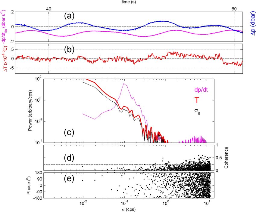
H. van Haren et al.: Diapycnal mixing across the photic zone of the NE Atlantic                                               303

phosphate) or at 4 ◦ C (silicate) until analysis. Nutrients were   2.1   Instrumentation and modification
analysed under temperature-controlled conditions using a
QuAAtro gas segmented continuous flow analyser. All mea-           Calibrated SeaBird 911plus CTD instruments were used. The
surements were calibrated with standards diluted in low-           CTD data were sampled at a rate of 24 Hz, whilst lowering
nutrient seawater in the salinity range of the stations to en-     the instrumental package at an average speed of 0.9 m s−1 .
sure that analysis remained within the same ionic strength.        The yo-yo CTD data were processed using the standard pro-
Phosphate (PO4 ) and nitrate plus nitrite (NOx ) were mea-         cedures incorporated in the SBE software, including correc-
sured according to Murphy and Riley (1962) and Grasshoff           tions for cell thermal mass (Lueck, 1990) using the param-
et al. (1983), respectively. Silicate was analysed using the       eter setting of Mensah et al. (2009), sensor time alignment
procedure of Strickland and Parsons (1968).                        and vertical bin averaging over 0.33 m. All other analyses
   Absolute and relative precision were regularly determined       were performed using Conservative Temperature (2), Ab-
for reasonably high concentrations in an in-house standard.        solute Salinity SA , and potential density anomalies σθ , with
For phosphate, the SD was 0.028 µM (N = 30) for a concen-          1000 kg m−3 subtracted from total density and referenced to
tration of 0.9 µM; hence the relative precision was 3.1 %. For     the surface for pressure corrections as only vertical profiles
nitrate, the values were 0.14 µM (N = 30) for a concentration      shallower than 600 m were analysed, using the Gibbs Sea-
of 14.0 µM, so that the relative precision was 1.0 %. For sili-    Water software (IOC, SCOR, IAPSO, 2010).
cate, the values were 0.09 µM (N = 15) for a concentration of         Observations were made with the yo-yo CTD instrument
21.0 µM, so that the relative precision was 0.4 %. The detec-      upright rather than horizontal in a lead-weighted frame with-
tion limits were 0.007, 0.012, and 0.008 µM, for phosphate,        out water samplers to minimize artificial turbulent over-
nitrate, and silicate, respectively.                               turning. Variable speeds of the flow passing the tempera-
   For dissolved iron samples, the ultraclean “pristine” sam-      ture and conductivity sensors will cause artificial temper-
pling system for trace metals was used (Rijkenberg et al.,         ature and thus apparent turbulent overturning, noticeable
2015). All bottles used for storage of reagents and sam-           in near-homogeneous waters such as those found near the
ples were cleaned according to an intensive three-step clean-      surface during nighttime convection. To eliminate variable
ing protocol described by Middag et al. (2009). Dissolved          flow speeds, a custom-made assembly with pump in- and
iron concentrations were measured shipboard using a flow-          outlet tubes and tube ends of exactly the same diameter
injection–chemiluminescence method with preconcentration           was mounted on the CTD instrument as described in van
on iminodiacetic acid resin as described by De Baar et al.         Haren and Laan (2016). This reduces frictional temperature
(2008) and modified by Klunder et al. (2011). In order to          effects of typically ± 0.5 mK due to fluctuations in pump
validate the accuracy of the system, standard reference sea-       speed of ± 0.5 m s−1 when standard SBE tubing is used (Ap-
water (SAFe) was measured regularly in triplicate (Johnson         pendix A). The effective removal of the artificial temperature
et al., 1997).                                                     effects using the custom-made assembly is demonstrated in
   At 19 out of 32 stations a yo-yo consisting of three to         Fig. 2, in which surface wave action via ship motion is visible
six casts, totaling 88 casts, of electronic CTD profiles was       in the CTD–pressure record but not in its temperature varia-
done to monitor the temperature–salinity variability and to        tions record. For example, at station 32 the CTD instrument
establish turbulent mixing values from 5 to 500 m below the        was lowered in moderate sea-state conditions with maximum
ocean surface. For the yo-yos a separate CTD instrument was        surface waves of 2 m crest trough. The surface waves are
used from the CTD ultraclean sampling system. The yo-yo            recorded by pressure variations as a result of ship motions
casts were made consecutively and took between 1 and 2 h           (Fig. 2a). In the upper 35 m near the surface, the waters were
per station. They were mostly obtained in the morning: at 10       partially unstable and partially near-homogeneous, with tem-
stations between 06:00 and 08:00 LT, at 8 stations between         perature variations well within ± 0.5 mK and high-frequency
08:00 and 10:00 LT, and at 1 station around noon. As the ob-       variations O(0.1) mK (Fig. 2b). The 1T variations did not
servations were made in summer, the latitudinal difference         vary with the surface wave periodicity of about 10 s. No cor-
in sunrise was 1.5 h between the northernmost (earlier sun-        relation was found between data in Fig. 2b and a. This effec-
rise) and southernmost stations. This difference is taken into     tive removal of ship motion in CTD temperature data is con-
account and sampling times are referenced to time after lo-        firmed for the entire 500 m depth range in average spectral
cal sunrise. It is assumed that the stations sampled just after    information (Fig. 2c–e). In the power spectra, the pressure
sunrise reflect the upper-ocean conditions of (late-) nighttime    gradient dp/dt ∼ CTD velocity shows a clear peak around
cooling convection so that vertical near-homogeneity was at        0.1 cps, short for cycles per second, which corresponds to a
a maximum and near-surface stratification at a minimum,            period of 10 s. Such a peak is absent in both spectra of tem-
while the late morning and afternoon stations reflected day-       perature T and density anomaly referenced to the surface σθ .
time stratifying near-surface conditions due to the stabilizing    The correlation between dp/dt and T is not significantly dif-
solar insolation.                                                  ferent from zero (Fig. 2d and e). With conventional tubing
                                                                   and tube ends, the surface wave variations would show up
                                                                   in such 1T graph (van Haren and Laan, 2016). Without the

https://doi.org/10.5194/os-17-301-2021                                                           Ocean Sci., 17, 301–318, 2021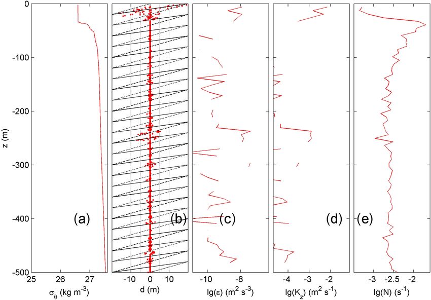
304                                           H. van Haren et al.: Diapycnal mixing across the photic zone of the NE Atlantic

Figure 2. Test of effective removal of ship motions in CTD data after pump in- and outlet modification. Nearly raw 24 Hz sampled downcast
data obtained from northern station 32 (cast 9). Short example time series for the 20 m depth range [10, 30] m. (a) Detrended pressure (blue)
and its (negative signed) first time derivative −dp/dt, 2 dbar smoothed (purple). (b) Detrended temperature. (c) Moderately smoothed (∼ 30
degrees of freedom; dof) spectra of data from the 5 to 500 m depth range. (d) Moderately smoothed (40 dof) coherence between dp/dt and T
from (c), with dashed line indicating the 95 % significance level. (e) Corresponding phase difference.

effects of ship motions, considerably less corrections need to           value LT = rms(d) computed over certain vertical scales (see
be applied for turbulence calculations (see below).                      below):

                                                                         ε = 0.64L2T N 3    [m2 s−3 ],                                   (1)
2.2   Ocean turbulence calculation
                                                                         where N = {−g/ρ(dσθ (zs )/dz)}1/2 denotes the buoyancy
Turbulence is quantified using the analysis method by Thorpe             frequency (∼ square root of stratification as is clear from
(1977) on potential density inversions of less dense water               the equation) computed from the reordered profile. Here,
below a layer of denser water in a vertical (z) profile. Such            g is the acceleration of gravity and ρ = 1027 kg m−3 de-
inversions are interpreted as turbulent overturns of mechan-             notes the reference density. We like to note, following pre-
ical energy mixing. Vertical turbulent kinetic energy dissi-             vious warnings by, e.g., Gill (1982) and King et al. (2012),
pation rate (ε) is a measure of the amount of kinetic en-                that our definition of N is a practical one, which should
ergy put in a system for turbulent mixing. It is proportional            not be used for data from deeper waters. For deeper wa-
to the magnitude of turbulent diapycnal flux (of potential               ters, density should be referenced to a local pressure refer-
density) |Kz dσθ /dz|. In practice it is determined by calcu-            ence level, which effectively implies the use of the exact def-
lating overturning scales with magnitude |d|, just like tur-             inition for buoyancy frequency as formulated by, e.g., Gill
bulent eddy diffusivity (Kz ). The vertical potential density            (1982): {−g/ρ(dρ/dz + gρ/cs2 )}1/2 , where cs is the speed of
stratification is indicated by dσθ /dz. The turbulent over-              sound reflecting pressure–compressibility effects. Our “sur-
turning scales are obtained after reordering the measured                face waters” N computed over reordered profiles only neg-
profile σθ (z), which may contain inversions, into a stable              ligibly deviates from above exact N and corresponds to N
monotonic profile σθ (zs ) without inversions (Thorpe, 1977).            computed from raw profiles over a typical vertical length
After comparing raw and reordered profiles, displacements                scale of 1z = 100 m. This 1z represents the scales of large
d = min(|z − zs |) · sgn(z − zs ) are calculated that generate the       internal waves that are supported by the density stratification
stable profile. Then, using root-mean-square displacement                and of the largest turbulent overturns.

Ocean Sci., 17, 301–318, 2021                                                                  https://doi.org/10.5194/os-17-301-2021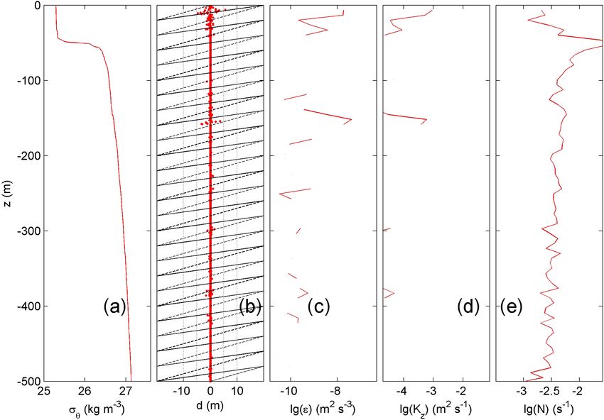
H. van Haren et al.: Diapycnal mixing across the photic zone of the NE Atlantic                                               305

   The numerical constant of 0.64 in Eq. (1) follows from         3     Results
empirically relating the overturning scale magnitude with the
Ozmidov scale LO of the largest possible turbulent over-          3.1    Physical parameters
turn in a stratified flow: (LO /LT ) = 0.8 (Dillon, 1982) this
is a mean coefficient value from many realizations. Using         An early morning vertical profile of density anomaly in
Kz = 0εN −2 and a mean mixing efficiency coefficient of           the upper 500 m at a northern station (Fig. 3a) is charac-
0 = 0.2 for the conversion of kinetic into potential energy for   terized by a near-homogeneous layer of about 15 to 40 m,
ocean observations that are suitably averaged over all rele-      which is above a layer of relatively strong stratification and
vant turbulent overturning scales of the mix of shear, current-   a smooth moderate stratification deeper below. In the near-
difference-driven and convective, buoyancy-driven overturn-       homogeneous upper layer, in this example z > −30 m, rel-
ing in large Reynolds number flow conditions (e.g. Osborn,        atively large turbulent overturn displacements can be found
1980; Oakey, 1982; Ferron et al., 1998; Gregg et al., 2018),      of d = ± 20 m (Fig. 3b): so-called large density inversions.
we find                                                           In this paper we conventionally define “mixed layer depth”
                                                                  as the depth at which the temperature difference with re-
Kz = 0.128L2T N[m2 s−1 ].                                  (2)    spect to the surface is 0.5 ◦ C (Jurado et al., 2012). We
                                                                  note that this actually more represents the “mixing layer
   This parametrization is also valid for the upper ocean, as     depth” and the reordered profile shows non-zero stratifica-
has been shown extensively by Oakey (1982) and recently           tion. If the mixed-layer-depth definition had been apply-
confirmed by Gregg et al. (2018). The inference is that the       ing a temperature difference of, e.g., 0.001 ◦ C on the re-
upper ocean may be weakly stratified at times, but stratifi-      ordered profile, its value would have averaged about 5 m,
cation and turbulence vary considerably with time and space.      much less than using the present and more common, conven-
Sufficient averaging collapses coefficients to the mean values    tional definition applying a temperature difference of 0.5 ◦ C.
given above. This is confirmed in recent numerical modelling      We thus present turbulence results for this commonly defined
by Portwood et al. (2019).                                        “mixed layer” with caution, whilst observing their consis-
   As Kz is a mechanical turbulence coefficient, it is not        tency with the results from deeper down, as presented be-
property-dependent like a molecular diffusion coefficient         low. For −200 < z < −30 m, large turbulent overturns are
that is about 100-fold different for temperature compared to      few and far between. Turbulence dissipation rate (Fig. 3c)
salinity. Kz is thus the same for all turbulent transport cal-    and eddy diffusivity (Fig. 3d) are characterized by relatively
culations no matter what gradient of what property. For ex-       small displacement sizes of less than 5 m. For z < −200 m,
ample, the vertical downgradient turbulent flux of dissolved      displacement values weakly increase with depth, together
iron transporting from iron-rich deeper waters upwards into       with stratification (∼ N 2 ; Fig. 3e). Between −30 < z < 0 m,
the euphotic zone is computed as −Kz d(DFe)/dz.                   turbulence dissipation rate values between our minimum de-
   According to Thorpe (1977), results from Eqs. (1) and (2)      tectable level 10−11 and > 10−8 m2 s−3 are similar to those
are only useful after averaging over the size of a turbulent      found by others, using microstructure profilers (e.g. Oakey,
overturn instead of using single displacements. Here, rms-        1982; Gregg, 1989), lowered acoustic Doppler current pro-
displacement values LT are not determined over individual         filer, or CTD Thorpe-scale analysis (e.g. Ferron et al., 1998;
overturns, as in Dillon (1982), but over 7 m vertical intervals   Walter et al., 2005; Kunze et al., 2006). Here, eddy diffu-
(equivalent to about 200 raw data samples) that just exceed       sivities are found between our minimum detectable 2 × 10⁻⁵
average LO . This avoids the complex distinction of smaller       and 3 × 10⁻³ m2 s−1 , and these values compare with previ-
overturns in larger ones and allows the use of a single length    ous near-surface results (Denman and Gargett, 1983). The
scale of averaging. As a criterion for determining overturns      relatively small |d| < 5 m displacements (Fig. 3b) are gen-
we only used those data of which the absolute value of dif-       uine turbulent overturns, and they resemble “Rankine vor-
ference with the local reordered value exceeds a threshold        tices”, a common model of cyclones (van Haren and Gosti-
of 7 × 10⁻⁵ kg m−3 , which comes from SDs of the potential        aux, 2014), as may be best visible in this example in the large
density profiles in near-homogeneous layers over 1 m inter-       turbulent overturn near the surface. The occasional erratic ap-
vals and which corresponds to noise-variational amplitudes        pearance in individual profiles, sometimes still visible in the
of 1.4 × 10⁻⁴ kg m−3 in raw data (e.g. Galbraith and Kel-         10-profile means, reflects smaller overturns in larger ones.
ley, 1996; Stansfield et al., 2001; Gargett and Garner, 2008).       A mid-morning profile at a southern station shows differ-
Vertically averaged turbulence values, short for averaged ε       ent characteristics (Fig. 4), although 500 m vertically aver-
and Kz values from Eqs. (1) and (2), can be calculated to         aged turbulence values are similar to within 10 % of those
within an error of a factor of 2 to 3, approximately. As will     of the northern station. This 10 % variation is well within
be demonstrated below, this is considerably less spread in        the error bounds of about a factor of 2. At this southern sta-
values than the natural turbulence values variability over typ-   tion, the near-surface layer is stably stratifying (Fig. 4a) and
ically 4 orders of magnitude at a given position and depth in     displays few overturning displacements (Fig. 4b), while the
the ocean (e.g. Gregg, 1989).                                     interior demonstrates rarer but occasional intense turbulent

https://doi.org/10.5194/os-17-301-2021                                                          Ocean Sci., 17, 301–318, 2021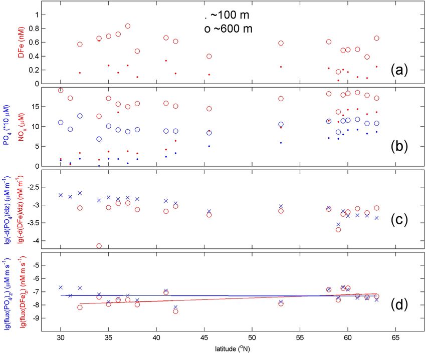
306                                            H. van Haren et al.: Diapycnal mixing across the photic zone of the NE Atlantic

Figure 3. Upper 500 m of turbulence characteristics computed from downcast density anomaly data applying a threshold of 7 × 10⁻⁵ kg m−3 .
Northern station 29, cast 2. (a) Unordered, “raw” profile of density anomaly referenced to the surface. (b) Overturn displacements following
reordering of the profiles in (a). Slopes 1/2 (solid lines) and 1 (dashed lines) are indicated. (c) Logarithm of dissipation rate computed from
the profiles in (a), rms calculated over 7 m intervals. We use the mathematics expression “lg” for the 10-base logarithm, as given in the ISO
80000 specification. (d) As (c), but for eddy diffusivity. (e) Logarithm of buoyancy frequency computed after reordering the profiles of (a).

Figure 4. As Fig. 3, but for a southern station. Upper 500 m of turbulence characteristics computed from downcast density anomaly data
applying a threshold of 7 × 10⁻⁵ kg m−3 . Southern station 3, cast 4. (a) Unordered, “raw” profile of density anomaly referenced to the
surface. (b) Overturn displacements following reordering of the profiles in (a). Slopes 1/2 (solid lines) and 1 (dashed lines) are indicated.
(c) Logarithm of dissipation rate computed from the profiles in (a), rms calculated over 7 m intervals. (d) As (c), but for eddy diffusivity.
(e) Logarithm of buoyancy frequency computed after reordering the profiles of (a).

Ocean Sci., 17, 301–318, 2021                                                                   https://doi.org/10.5194/os-17-301-2021
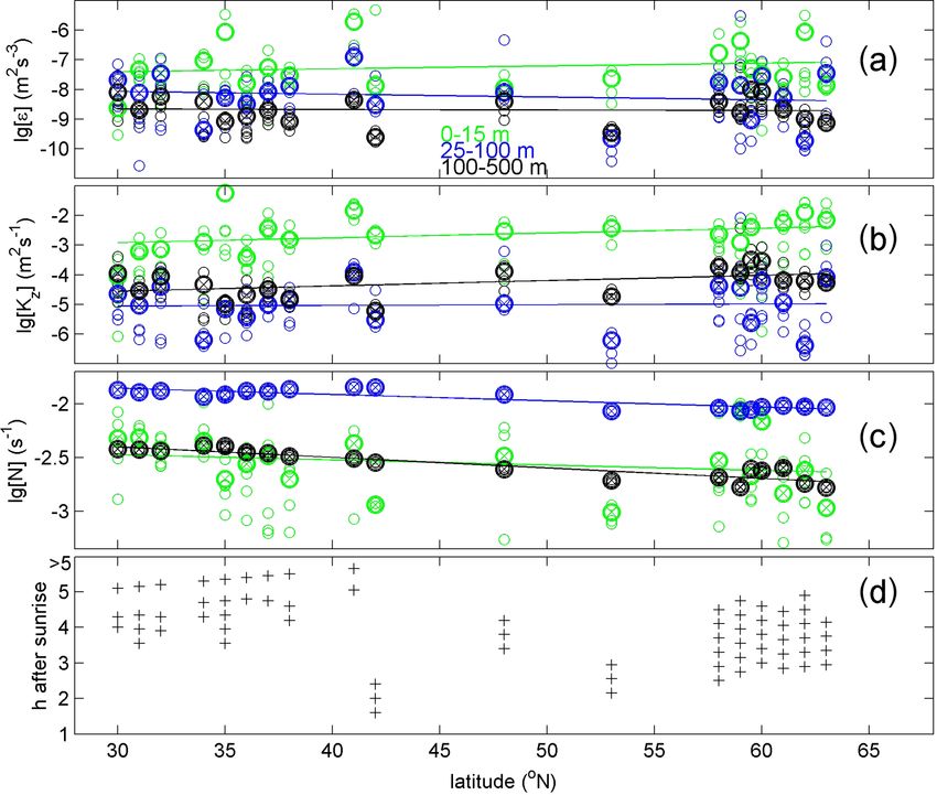
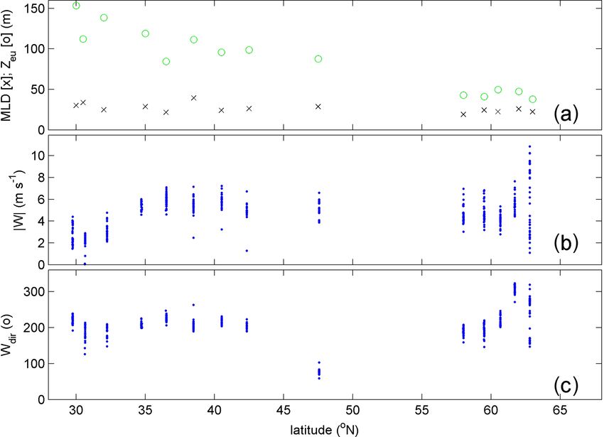
H. van Haren et al.: Diapycnal mixing across the photic zone of the NE Atlantic                                                  307

overturning (at z = −160 m in Fig. 4), presumably due to in-            Between −500 < z < −100 m, no clear significant trend
ternal wave breaking. At greater depths, stratification (∼ N 2 ;     with latitude is visible in the turbulence values (Fig. 5a
Fig. 4e) weakly decreases, together with ε (Fig. 4c) and Kz          and b), although [Kz ] weakly increases with increasing lati-
(Fig. 4d).                                                           tude at all levels between −500 < z < 0 m, while buoyancy
   Latitudinal overviews are given in Fig. 5 for (1) aver-           frequency significantly decreases (Fig. 5c). The data from
age values over the upper z > −15 m, which covers the di-            well-stratified waters deeper down thus show the same lat-
urnal mainly convective turbulent mixing range from the              itudinal trend as the observations from the near-surface lay-
surface and under the cautionary note that these waters are          ers, even though the latter are less well determined because of
weakly, but measurably stratified, (2) average values between        the weak stratification. Our turbulence values from CTD data
−100 < z < −25 m, which covers the seasonal strong stratifi-         also confirm previous results by Jurado et al. (2012), who
cation, and (3) average values between −500 < z < −100 m,            made microstructure profiler observations from the upper
which covers the more permanent moderate stratification.             z > −100 m along the same transect. Their results showed
Noting that all panels have a vertical axis representing a log-      turbulence values remain unchanged over 30◦ latitude or in-
arithmic scale, variations over nearly 4 orders of magnitude         crease by at most 1 order of magnitude, depending on depth
in turbulence dissipation rate (Fig. 5a) and eddy diffusiv-          level. Their mixed layer (z > ∼ −25 m) turbulence values are
ity (Fig. 5b) are observed between casts at the same station.        similar to our z > −15 m values and 0.5 to 1 order of magni-
This variation in magnitude is typically found in near-surface       tude larger than the present deeper observations. The slight
open-ocean turbulence microstructure profiles (e.g. Oakey,           discrepancy in values averaged over z > −25 m may point to
1982). Still, considerable variability over about 2 orders of        either (i) a low bias due to too strict a criterion of accepting
magnitude is observed between the averages from the differ-          density variations for reordering applied here or (ii) a high
ent stations. This variation in station and vertical averages far    bias of the ∼ 10 m largest overturns having similar veloc-
exceeds the instrumental error bounds of a factor of 2 (0.3 on       ity scales (of about 0.05 m s−1 ) as their 0.1 m s−1 slowly de-
a log scale) and thus reveals local variability. The turbulence      scending SCAMP (Self Contained Autonomous Microstruc-
processes occur “intermittently”.                                    ture Profiler). At greater depths (−500 < z < −100 m), it is
   The observed variability over 2 orders of magnitude be-           seen in the present observations that the spread in turbulence
tween yo-yo casts at a single station may be due to active           values over 4 orders of magnitude at a particular station is
convective overturning during early morning in the near-             also large. This spread in values suggests that dominant tur-
homogeneous upper layer or due to internal wave break-               bulence processes show similar intermittency in weakly (at
ing and sub-mesoscale variability deeper down. Despite the           high latitudes N ≈ 10−2.5 s−1 ) and moderately (at midlati-
large variability at stations, trends are visible between sta-       tudes N ≈ 10−2.2 s−1 ) stratified waters, respectively, for the
tions in the upper 100 m over the 33◦ latitudinal range going        given resolution of the instrumentation.
poleward: buoyancy frequency (∼ square root of stratifica-              Mean values of N are larger by 0.5 orders of mag-
tion) steadily decreases significantly (p value < 0.05) given        nitude in the seasonal pycnocline (found in the range
the spread of values at given stations, with the notion that         −100 < z < −25 m) than those near the surface and in the
near-surface (−15 < z < 0 m) values show the same latitudi-          more permanent stratification below (Fig. 5). Such local ver-
nal trend as deeper down values across a larger spread of            tical variations in N have the same range of variation as ob-
values, while turbulence values vary insignificantly with lat-       served horizontally across latitudes [30, 63]◦ per depth level.
itude as they remain the same or weakly increase by about
0.5 orders of magnitude (about a factor of 3). At a given            3.2   Nutrient distributions and fluxes
depth range, turbulence dissipation rates roughly follow a
log-normal distribution with SDs well exceeding 0.5 orders           Vertical profiles of macro-nutrients generally resemble those
of magnitude. The comparison of latitudinal variations with          of density anomaly in the upper z > −500 m (Fig. 6). In the
the (log-normal) distribution is declared insignificant with         south, low macro-nutrient values are generally distributed
p > 0.05 when the mean values are found within 2 SDs (see            over a somewhat larger near-surface mixed layer. The mixed
Appendix B). This is not only performed for turbulence dis-          layer depth, at which temperature differed by 0.5 ◦ C from
sipation rate but also for other quantities. The trends suggest      the surface (Jurado et al., 2012), varies between about 20
only marginally larger turbulence going poleward, which is           and 30 m on the southern end of the transect and weakly
possibly due to larger cooling from above and larger internal        becomes shallower with latitude (Fig. 7a). This weak trend
wave breaking deeper down. It is noted that the results are          may be expected from the summertime wind conditions that
somewhat biased by the sampling scheme, which changed                also barely vary with latitude (Fig. 7b and c). In contrast,
from 3 to 4 h after sunrise sampling at high latitudes to 4 to       the euphotic zone, defined as the depth of the 0.1 % irradi-
5 h after sunrise sampling at lower latitudes; see the sampling      ance penetration level (Mojica et al., 2015), demonstrates
hours after local sunrise in (Fig. 5d). Its effect is difficult to   a clear latitudinal trend decreasing from about 150 to 50 m
quantify but should not show up in turbulence values from            (Fig. 7a). For z < −100 m below the seasonal stratification,
deeper down (−500 < z < −100 m).                                     vertical gradients of macro-nutrients are large (Fig. 6b–d).

https://doi.org/10.5194/os-17-301-2021                                                             Ocean Sci., 17, 301–318, 2021
308                                            H. van Haren et al.: Diapycnal mixing across the photic zone of the NE Atlantic

Figure 5. Summer 2017 latitudinal transect along 17 ± 5◦ W of turbulence values for upper 15 m averages (green) and averages between
−100 < z < −25 m (blue, seasonal pycnocline) and −500 < z < −100 m (black, more permanent pycnocline) from short yo-yos of three
to six CTD casts. Values are given per cast (o) and station average (heavy circle with x; the size corresponds to ± the standard error for
turbulence parameters). (a) Logarithm of dissipation rate. (b) Logarithm of diffusivity. (c) Logarithm of buoyancy frequency (the small
symbols have the size of ± the standard error). (d) Hour of sampling after sunrise.

Figure 6. Upper 500 m profiles for stations at three latitudes. (a) Density anomaly referenced to the surface, including profiles from Figs. 3a
and 4a. (b) Nitrate plus nitrite. (c) Phosphate. (d) Silicate. (e) Dissolved iron.

Ocean Sci., 17, 301–318, 2021                                                                   https://doi.org/10.5194/os-17-301-2021
H. van Haren et al.: Diapycnal mixing across the photic zone of the NE Atlantic 309
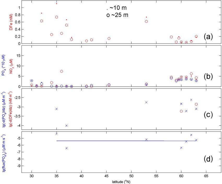
Figure 7. Latitudinal transect of near-surface layers and wind conditions measured at stations during the observational survey. (a) Mixed
layer depth (x) and euphotic zone (o). (b) Wind speed. (c) Wind direction.
Macro-nutrient values become approximately independent of ambiguously or statistically independently varying with lati-
latitude at depths below z < −500 m. Dissolved iron profiles tude (Fig. 9d). Likewise, the vertical turbulent fluxes of dis-
differ from macro-nutrient profiles, notably in the upper layer solved iron and phosphate are marginally constant with lat-
near the surface (Fig. 6a). At some southern stations, dis- itude across the more permanent stratification deeper down
solved iron and to a lesser extent also phosphate have rela- (Fig. 10). Nitrate fluxes show the same latitudinal trend, with
tively high concentrations closest to the surface. These near- values around 10−6 mmol m−2 s−1 . Overall, the vertical tur-
surface concentration increases suggest atmospheric sources, bulent nutrient fluxes across the seasonal and more perma-
most likely Saharan dust deposition (e.g. Rijkenberg et al., nent stratification resemble those of the physical vertical tur-
2012). bulent mass flux, which is equivalent to the distribution of
As a function of latitude in the near-surface mixed layer turbulence dissipation rate and which is latitude invariant
(Fig. 8), the vertical turbulent fluxes of phosphate (represent- (Fig. 5a).
ing the macro-nutrients, for graphical reasons; see the simi-
larity in profiles in Fig. 6b–d) are found to be constant or in-
significantly (p > 0.05) increasing (Fig. 8d). Here, the mean 4 Discussion
eddy diffusivity values for the near-surface layer as presented
in Fig. 5 are used for computing the fluxes. It is noted that in Practically, the upright positioning of the CTD instrument
this layer turbulent overturning (Figs. 3b and 4b) is larger while using an adaptation consisting of a custom-made
and nutrients are mainly depleted (Fig. 6), except when re- equal-surface inlet worked well to minimize ship-motion ef-
plenished from atmospheric sources, in which case gradi- fects on variable flow-imposed temperature variations. This
ents reverse sign as in most DFe profiles. Hereby, lateral improved calculated turbulence values from CTD observa-
diffusion is not considered important. Nonetheless, macro- tions in general and in near-homogeneous layers in partic-
nutrients are seen to increase significantly towards higher lat- ular. The indirect comparison with turbulence values de-
itudes (Fig. 8b). We note that the vertical gradients in Fig. 8c, termined from previous microstructure profiler observations
in which only downgradient values are plotted, are very weak along the same transect (Jurado et al., 2012) confirms the
in general within the SD of measurements. The results in same trends, although occasionally turbulence values were
Fig. 8d are thus merely indicative, but they are consistent lower (to 1 order of magnitude in the present study). This
with the results from deeper down presented below. difference in values may be due to the time lapse of 8 years
More importantly, the significant vertical turbulent fluxes between the observations, but more likely it is due to inac-
of nutrients across the seasonal pycnocline (Fig. 9) are found curacies in one or both methods. It is noted that any ocean
turbulence observations cannot be made better than to within
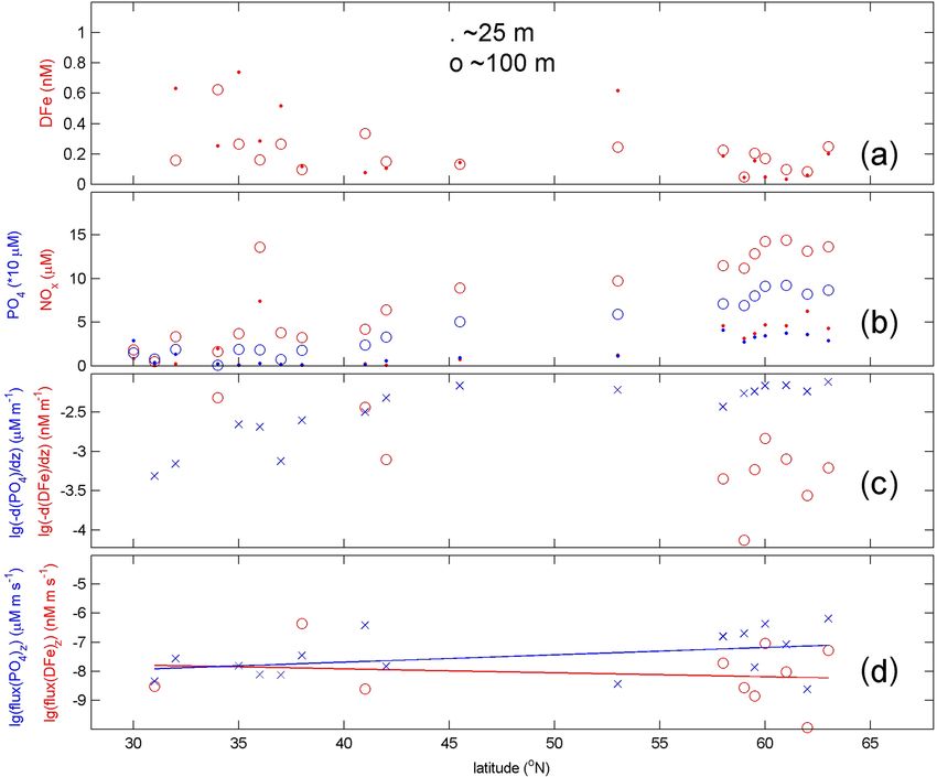
https://doi.org/10.5194/os-17-301-2021 Ocean Sci., 17, 301–318, 2021310 H. van Haren et al.: Diapycnal mixing across the photic zone of the NE Atlantic Figure 8. Latitudinal transect of near-surface nutrient concentrations. (a) Dissolved iron measured at depths indicated. Missing values reflect that not all depths were sampled. (b) Nitrate plus nitrite (red) and phosphate (blue, scale times 10) measured at depths indicated in (a). (c) Logarithm of (very weak within SDs of measurements) vertical gradients of dissolved iron in (a) (o, red) and phosphate in (b) (x, blue). Only downgradient values are shown, which excludes several PO4 - and nearly all DFe-gradient values due to near-surface increased values (cf. Fig. 6e, 32◦ N profile). (d) Upward vertical turbulent fluxes of phosphate concentration gradients in (c). Using average surface Kz from Fig. 5b, valid for depth average (here, ∼ 17 m) of depths in (a). a factor of 2 (Neil Oakey, personal communication, 1991). In future research may perform a more extensive comparison that respect, the standard CTD instrument with the adapta- between Thorpe-scale analysis data and deeper microstruc- tion presented here is a cheaper solution than additional mi- ture profiler data. crostructure profiler observations. Although the general un- While our turbulence values are roughly similar to those derstanding, mainly amongst modellers, is that the Thorpe of others transecting the NE Atlantic over the entire water length method overestimates diffusivity (e.g. Scotti, 2015; depth (Walter et al., 2005; Kunze et al., 2006), the focus in Mater et al., 2015), this view is not shared amongst ocean the present paper is on the upper 500 m because of its im- observers (e.g. Gregg et al., 2018). In the large parame- portance for upper-ocean marine biology. Our study demon- ter space of the high Reynolds number environment of the strates a significant decrease in stratification with increasing ocean, turbulence properties vary constantly, with an inter- latitude and decreasing temperature that, however, does not mingling of convection and shear-induced turbulence at var- lead to significant variation in turbulence values and vertical ious levels. Given sufficient averaging and adequate mean turbulent fluxes. Our direct estimates of the turbulent flux of value parametrization, the Thorpe length method is not ob- nitrate into the euphotic zone are 1 to 2 orders of magnitude served to overestimate diffusivity. This property of adequate less than the previously estimated rate of nitrate uptake for and sufficient averaging yields similar mean parameter val- the summer period. Our turbulent flux of nitrate values are ues in recent modelling results estimating a mixing coeffi- of the same order of magnitude as reported by others (Cyr cient near the classical bound of 0.2 in stationary flows for a et al., 2015, and references therein). In particular, the Mar- wide range of conditions (Portwood et al., 2019). It is noted tin et al. (2010) study in the northeast Atlantic Ocean (at that diffusivity always requires knowledge of stratification to 49◦ N, 16◦ W) reported similar vertical nutrient fluxes dur- obtain a turbulent flux, and it is better to consider turbulence ing summer, which provides confidence in the methods used. dissipation rate for intercomparison purposes. Nevertheless, The same authors reported that the vertical nitrate flux into Ocean Sci., 17, 301–318, 2021 https://doi.org/10.5194/os-17-301-2021
H. van Haren et al.: Diapycnal mixing across the photic zone of the NE Atlantic                                                     311

Figure 9. As Fig. 8, but for −100 < z < −25 m, with fluxes for ∼ 62 m in (d).

the euphotic zone was much lower than the rate of nitrate               despite the relatively slow turbulence compared to surface
update at the time. To determine these nitrate uptake rates,            wave breaking. Depending on the gradient of a substance like
they spiked water samples with a minimum of 0.5 µM nitrate,             nutrients or matter, the relatively slow turbulence may not
representing ∼ 10 % of the ambient nitrate concentration. In            necessarily provide weak fluxes −Kz d(substance)/dz into
our study area, the ambient nitrate concentrations in the eu-           the photic zone. In the central North Sea, a relatively low
photic zone were much lower (see also Mojica et al., 2015),             mean value of Kz = 2 × 10⁻⁵ m2 s−1 , comparable to values
implying a higher relative importance of nitrate input to the           over the seasonal pycnocline here, was found sufficient to
overall uptake demand. Still, primary productivity in the olig-         supply nutrients across the strong summer pycnocline to sus-
otrophic euphotic zone, as well as in the high-latitude At-             tain the entire late-summer phytoplankton bloom in near-
lantic, is mainly fuelled by recycling (e.g. Gaul et al., 1999;         surface waters and to warm up the near-bottom waters by
Achterberg et al., 2020), and the supply of new nutrients by            some 3 ◦ C over the period of seasonal stratification (van
turbulent fluxes, however small, provides a welcome addi-               Haren et al., 1999). There, the turbulent exchange was driven
tion. Besides nutrient input resulting from vertical turbulent          by a combination of tidal currents modified by the stratifica-
fluxes, there is a role for latitudinal differences through the         tion and shear by inertial motions driven by the Coriolis force
supply of nutrients by deep mixing events and, depending                (inertial shear) and internal wave breaking. Such drivers are
on the location, also potential upwelling and lateral transport         also known to occur in the open ocean, although to an un-
events.                                                                 known extent.
   We suggest that internal waves may drive the feedback                   The here observed (lack of) latitudinal trends of ε, Kz , and
mechanism, participating in the subtle balance between                  N yield approximately the same information as the vertical
destabilizing shear and stable (re)stratification. Molecular            trends in these parameters at all stations. In the vertical for
diffusivity of heat is about 10−7 m2 s−1 in seawater and                z < −200 m, turbulence values of ε and Kz weakly vary with
nearly always smaller than turbulent diffusivity in the ocean.          stratification. This is perhaps unexpected and contrary to the
The average values of Kz during our study were typically                common belief of stratification hampering vertical turbulent
100 to 1000 times larger than molecular diffusivity, which              exchange of matter including nutrients. It is less surprising
implies that turbulent diapycnal mixing drives vertical fluxes          when considering that increasing stratification is able to sup-

https://doi.org/10.5194/os-17-301-2021                                                                Ocean Sci., 17, 301–318, 2021
312                                          H. van Haren et al.: Diapycnal mixing across the photic zone of the NE Atlantic

Figure 10. As Fig. 8, but for −600 (few nutrients sampled at 500) < z < −100 m, with fluxes for ∼ 350 m in (d).

port larger shear. Known sources of destabilizing shear in-            )mesoscale activities are energetically very different across
clude near-inertial internal waves of which the vertical length        the midlatitudes. If internal tide sources had dominated our
scale is relatively small compared to other internal waves, in-        observations, clear differences in turbulence dissipation rates
cluding internal tides (LeBlond and Mysak, 1978).                      would have been found at our station near 48◦ N (near the
   The dominance of inertial shear over shear by internal tidal        Porcupine Bank), for example, compared with those at other
motions (internal tide shear), together with larger energy in          stations.
the internal tidal waves, has been observed in the open ocean,            Summarizing, our study infers that vertical nutrient fluxes
e.g. in the Irminger Sea around 60◦ N (van Haren, 2007). The           did not vary significantly with latitude and stratification. This
frequent atmospheric disturbances in that area generate iner-          suggests that predicted changes in the physical environment
tial motions and dominant inertial shear. Internal tides have          due to global ocean warming have little effect on vertical tur-
larger amplitudes, but due to much larger length scales they           bulent exchange. Supposing that enhanced warming leads to
generate weaker shear than inertial motions. Small-scale in-           more stable stratification, more internal waves can be sup-
ternal waves near the buoyancy frequency are abundant and              ported (LeBlond and Mysak, 1978), which upon breaking
may break sparsely in the ocean interior outside regions of to-        can maintain the extent of vertical turbulent exchange and
pographic influence. However, larger destabilizing shear re-           thereby, for example, vertical nutrient fluxes. We thus hy-
quires larger stable stratification to attain a subtle balance of      pothesize that, from a physical environment perspective, in
“constant” marginal stability (van Haren et al., 1999). Not            stratified oligotrophic waters the nutrient input from deeper
only storms but all geostrophic adjustments, such as frontal           waters and corresponding summer phytoplankton productiv-
collapse, may generate inertial wave shear also at low lat-            ity and growth are not expected to change (much) with future
itudes (Alford and Gregg, 2001), so that overall latitudinal           global warming. We invite future observations and numerical
dependence may be negligible. If shear-induced turbulence              modelling to further investigate this suggestion and associ-
in the upper ocean is dominant, it may thus be latitudinally           ated feedback mechanisms such as internal wave breaking.
independent (shallow observations by Jurado et al., 2012;
deeper observations in present study). There are no indica-
tions that the overall open-ocean internal wave field and (sub-

Ocean Sci., 17, 301–318, 2021                                                                https://doi.org/10.5194/os-17-301-2021
H. van Haren et al.: Diapycnal mixing across the photic zone of the NE Atlantic                                                  313

Appendix A: Modification of CTD pump tubing to
minimize hydrodynamic ram effects

The unique pump system on SeaBird Electronics (SBE)
CTD instruments, foremost on their high-precision full ocean
depth shipborne and cable-lowered SBE911, minimizes the
effects of flow variations (and inversions) past its T–C sen-
sors (SeaBird, 2012). This reduction in flow variation is im-
portant because the T sensor has a slower response than the C
sensor. As data from the latter are highly temperature depen-
dent, besides being pressure dependent, the precise matching
of all three sensors is crucial for establishing proper salinity
and density measurements, especially across rapid changes
in any of the parameters. As flow past the T sensor causes
higher measurement values due to friction at the sensor tip,
flow fluctuations are to be avoided as they create artificial T
variations of about 1 mK s m−1 (Larson and Pedersen, 1996).
   However, while the pump itself is one thing, its tubing
needs careful mounting as well, with the in- and outlet at
the same depth level (Sea-Bird, 2012). This is to prevent ram
pressure P = ρU 2 , for density ρ and flow speed U . Unfor-
tunately, the SBE manual shows tubing of different diam-
eters, for in- and outlet. Different diameter tubing leads to
velocity fluctuations of ± 0.5 m s−1 past the T sensor, as was
concluded from a simple experiment by van Haren and Laan
(2016). The flow speed variations induce temperature varia-
tions of ± 0.5 mK and are mainly detectable in weakly strati-
fied waters such as in the deep ocean but also near the surface
as observed in the present data. Using tubes of the same di-
ameter opening counteracted most of the effect, but only if
the surface of the tube opening is perpendicular to the main
CT motion as in a vertically mounted CTD instrument. If it is
parallel to the main motion as in a horizontally mounted CTD
instrument, the effect was found to be adverse. The make-
shift onboard experiment in van Haren and Laan (2016) has
now been cast into a better design (Fig. A1), of which the
first results are presented in this paper.

                                                                   Figure A1. SBE911 CTD pump in- and outlet modification follow-
                                                                   ing the findings in van Haren and Laan (2016). (a) The T and C sen-
                                                                   sors clamped together with a structure holding in- and outlet pump
                                                                   tubing of exactly the same diameter, separated at 0.3 m distance in
                                                                   the horizontal plane. (b) The modification of (a) mounted in the
                                                                   CTD frame.

https://doi.org/10.5194/os-17-301-2021                                                             Ocean Sci., 17, 301–318, 2021
314 H. van Haren et al.: Diapycnal mixing across the photic zone of the NE Atlantic
Appendix B: PDFs of vertically averaged dissipation When we compare the mean and SDs of the distributions
rate in comparison with latitudinal trends with the extreme values of the latitudinal trends as computed
for Fig. 5a it is seen that the extreme values are not found
Ocean turbulence dissipation rate generally tends to a nearly outside 1 SD from the mean value for any of the three depth
log-normal distribution (e.g. Pearson and Fox-Kemper, levels. In fact, for deeper stratified waters the extreme values
2018), so that the probability density function (PDF) of the of the trends are found very close to the mean value. It is
logarithm of ε values is normally distributed and can be de- concluded that the mean dissipation rate does not show a sig-
scribed by the first two moments, the mean, and its SD. It nificant trend with latitude, at all depth levels. The same exer-
is seen in Fig. B1 that the overall distribution of all present cise yields extreme buoyancy frequency values lying outside
data indeed approaches log-normality, despite the relatively 1 SD from the mean values for well-stratified waters, from
large length scale used in the computations (cf. Yamazaki and which we conclude that stratification significantly decreases
Lueck, 1990). When the data are split into the three depth lev- with latitude. This is inferable from Fig. 5c by investigating
els as in Fig. 5a, it is seen that ε in the upper z > −15 m layer the spread of mean values around the trend line.
is not log-normally distributed due to a few outlying high val-
ues confirming an ocean state dominated by a few turbulence
bursts (Moum and Rippeth, 2009), whereas ε in the deeper
more stratified layers is nearly log-normally distributed.
Ocean Sci., 17, 301–318, 2021 https://doi.org/10.5194/os-17-301-2021H. van Haren et al.: Diapycnal mixing across the photic zone of the NE Atlantic 315 Figure B1. Probability density functions of logarithm of the vertically averaged dissipation rate in comparison with latitudinal trend extreme values. (a) Distribution as a function of latitude for all data. (b) As (a), but for the upper 15 m averages only. The mean value is given by the vertical purple line, with the horizontal line indicating ± 1 SD. The vertical light-blue lines indicate the best-fit value of the trend for 30 and 63◦ N. (c) As (b), but for averages between −100 < z < −25 m. (d) As (c), but for averages between −500 < z < −100 m. https://doi.org/10.5194/os-17-301-2021 Ocean Sci., 17, 301–318, 2021
316                                            H. van Haren et al.: Diapycnal mixing across the photic zone of the NE Atlantic

Code availability. The data are available at                           Denman, K. L. and Gargett, A. E.: Time and space scales of verti-
https://doi.org/10.25850/nioz/7b.b.lb (van Haren et al., 2021). We        cal mixing and advection of phytoplankton in the upper ocean,
use chemical analyses and SeaBird 911 CTD SBEdataprocessing-              Limnol. Oceanogr., 28, 801–815, 1983.
Win32 software; the plots are made in Matlab 2014b. We do not          Dillon, T. M.: Vertical overturns: A comparison of Thorpe and
use a numerical model.                                                    Ozmidov length scales, J. Geophys. Res., 87, 9601–9613, 1982.
                                                                       Ferron, B., Mercier, H., Speer, K., Gargett, A., and Polzin, K.:
                                                                          Mixing in the Romanche Fracture Zone, J. Phys. Oceanogr., 28,
Data availability. Data are available under                               1929–1945, 1998.
https://doi.org/10.25850/nioz/7b.b.lb (van Haren et al., 2021).        Galbraith, P. S. and Kelley, D. E.: Identifying overturns in CTD pro-
                                                                          files, J. Atmos. Ocean. Tech., 13, 688–702, 1996.
                                                                       Gargett, A. and Garner, T.: Determining Thorpe scales from ship-
Author contributions. HvH analysed the data and drafted the paper.        lowered CTD density profiles, J. Atmos. Ocean. Tech., 25, 1657–
CPDB coordinated the cruise. RM, MHvM, and CPDB provided                  1670, 2008.
the nutrient and iron data. LJAG initiated the link of disciplines     Gaul, W., Antia, A. N., and Koeve, W.: Microzooplankton grazing
in this study and stored the datasets. RG handled and operated the        and nitrogen supply of phytoplankton growth in the temperate
CTD systems. All authors contributed to the scientific discussion         and subtropical northeast Atlantic, Mar. Ecol. Prog. Ser., 189,
and edited the paper. All authors have read and agreed to the pub-        93–104, 1999.
lished version of the paper.                                           Gill, A. E.: Atmosphere-Ocean Dynamics, Academic Press, Or-
                                                                          lando, Fl, USA, 662 pp., 1982.
                                                                       Grasshoff, K., Kremling, K., and Ehrhardt, M.: Methods of seawater
                                                                          analysis, Verlag Chemie GmbH, Weinheim, 419 pp., 1983.
Competing interests. The authors declare that they have no conflict
                                                                       Gregg, M. C.: Scaling turbulent dissipation in the thermocline, J.
of interest.
                                                                          Geophys. Res., 94, 9686–9698, 1989.
                                                                       Gregg, M. C., Sanford, T. B., and Winkel, D. P.: Reduced mixing
                                                                          from the breaking of internal waves in equatorial waters, Nature,
Acknowledgements. We thank the master and crew of the R/V Pela-           422, 513–515, 2003.
gia for their pleasant contributions to the sea operations. Jo-        Gregg, M. C., D’Asaro, E. A., Riley, J. J., and Kunze, E.: Mixing
han van Heerwaarden and Roel Bakker made the CTD modification.            efficiency in the ocean, Annu. Rev. Mar. Sci., 10, 443–473, 2018.
We much appreciated the critical comments of the reviewers.            Henyey, F. S., Wright, J., and Flatte, S. M.: Energy and action flow
                                                                          through the internal wave field – an eikonal approach, J. Geo-
                                                                          phys. Res., 91, 8487–8495, 1986.
Review statement. This paper was edited by Ilker Fer and reviewed      Hernández-Hernández, N., Arístegui, J., Montero, M. F., Velasco-
by three anonymous referees.                                              Senovilla, E., Baltar, F., Marrero-Díaz, Á., Martínez-Marrero,
                                                                          A., and Rodríguez-Santana, Á.: Drivers of plankton distribution
                                                                          across mesoscale eddies at submesoscale range, Front. Mar. Sci.,
                                                                          7, 667, https://doi.org/10.3389/fmars.2020.00667, 2020.
References                                                             Hibiya, T., Nagasawa, M., and Niwa, Y.: Latitudinal depen-
                                                                          dence of diapycnal diffusivity in the thermocline observed us-
Achterberg, E. P., Steigenberger, S., Klar, J. K., Browning, T. J.,       ing a microstructure profiler, Geophys. Res. Lett., 34, L24602,
  Marsay, C. M., Painter, S. C., Vieira, L. H., Baker, A. R., Hamil-      https://doi.org/10.1029/2007GL032323, 2007.
  ton, D. S., Tanhua, T., and Moore, C. M.: Trace element bio-         Huisman, J., Pham Thi, N. N., Karl, D. M., and Sommeijer, B.:
  geochemistry in the high latitude North Atlantic Ocean: sea-            Reduced mixing generates oscillations and chaos in the oceanic
  sonal variations and volcanic inputs, Global Biogeochem. Cy.,           deep chlorophyll maximum, Nature, 439, 322–325, 2006.
  https://doi.org/10.1029/2020GB006674, in press, 2020.                IOC, SCOR, IAPSO: The international thermodynamic equation of
Alford, M. H. and Gregg, M. C.: Near-inertial mixing: Modulation          seawater – 2010: Calculation and use of thermodynamic prop-
  of shear, strain and microstructure at low latitude, J. Geophys.        erties, Intergovernmental Oceanographic Commission, Manuals
  Res., 106, 16947–16968, 2001.                                           and Guides No. 56, UNESCO, Paris, France, 196 pp., 2010.
Charria, G., Theetten, S., Vandermeirsch, F., Yelekçi, Ö., and         Johnson, K. S., Gordon, R. M., and Coale, K. H.: What controls
  Audiffren, N.: Interannual evolution of (sub)mesoscale dy-              dissolved iron concentrations in the world ocean?, Mar. Chem.,
  namics in the Bay of Biscay, Ocean Sci., 13, 777–797,                   57, 137–161, 1997.
  https://doi.org/10.5194/os-13-777-2017, 2017.                        Jurado, E., van der Woerd, H. J., and Dijkstra, H. A.: Microstruc-
Cyr, F., Bourgault, D., Galbraith, P. S., and Gosselin,                   ture measurements along a quasi-meridional transect in the
  M.: Turbulent nitrate fluxes inthe Lower St. Lawrence                   northeastern Atlantic Ocean, J. Geophys. Res., 117, C04016,
  Estuary, Canada, J. Geophys. Res., 120, 2308–2330,                      https://doi.org/10.1029/2011JC007137, 2012.
  https://doi.org/10.1002/2014JC010272, 2015.                          King, B., Stone, M., Zhang, H. P., Gerkema, T., Marder, M., Scott,
De Baar, H. J. W., Timmermans, K. R., Laan, P., De Porto, H. H.,          R. B., and Swinney, H. L.: Buoyancy frequency profiles and in-
  Ober, S., Blom, J. J., Bakker, M. C., Schilling, J., Sarthou, G.,       ternal semidiurnal tide turning depths in the oceans, J. Geophys.
  Smit, M. G., and Klunder, M.: Titan: A new facility for ultraclean      Res., 117, C04008, https://doi.org/10.1029/2011JC007681,
  sampling of trace elements and isotopes in the deep oceans in the       2012.
  international Geotraces program, Mar. Chem., 111, 4–21, 2008.

Ocean Sci., 17, 301–318, 2021                                                                https://doi.org/10.5194/os-17-301-2021
You can also read