SIRENA: A CAD Environment for Behavioral Modeling and Simulation of VLSI Cellular Neural Network Chips
←
→
Page content transcription
If your browser does not render page correctly, please read the page content below
SIRENA: A CAD Environment for Behavioral Modeling and Simulation of VLSI Cellular Neural Network Chips

    SIRENA: A CAD Environment for Behavioral Modeling
    and Simulation of VLSI Cellular Neural Network Chips

R. Carmona, I. García-Vargas, G. Liñán, R. Domínguez-Castro, S. Espejo and A. Rodríguez-
                                        Vázquez
                Instituto de Microelectrónica de Sevilla-CNM-CSIC / Universidad de Sevilla
                              Edificio CICA, C/Tarfia sn, 41012-Sevilla, SPAIN
                                 Phone #34 5 4239923, FAX #34 5 4231832

                                               Abstract

       This paper presents SIRENA, a CAD environment for the simulation and modeling of
mixed-signal VLSI parallel processing chips based on Cellular Neural Networks. SIRENA
includes capabilities for: a) the description of nominal and non-ideal operation of CNN analog
circuitry at the behavioral level; b) performing realistic simulations of the transient evolution of
physical CNNs including deviations due to second-order effects of the hardware; and, c) evalu-
ating sensitivity figures, and realize noise and Montecarlo simulations in the time domain.
These capabilities portray SIRENA as better suited for CNN chip development than algorithmic
simulation packages (such as OpenSimulator, Sesame) or conventional Neural Networks simu-
lators (RCS, GENESIS, SFINX), which are not oriented to the evaluation of hardware non-ide-
alities. As compared to conventional electrical simulators (such as HSPICE or ELDO-FAS),
SIRENA provides easier modeling of the hardware parasitics, a significant reduction in compu-
tation time, and similar accuracy levels. Consequently, iteration during the design procedure
becomes possible, supporting decision making regarding design strategies and dimensioning.
SIRENA has been developed using object-oriented programming techniques in C, and currently
runs under the UNIX operating system and X-Windows framework. It employs a dedicated
high-level hardware description language: DECEL, fitted to the description of non-idealities
arising in CNN hardware. This language has been developed aiming generality, in the sense of
making no restrictions on the network models that can be implemented. SIRENA is highly mod-
ular and composed of independent tools. This simplifies future expansions and improvements.

Front-page Footnotes:
1
2

    1. This work has been partially funded by spanish CICYT under contract TIC96-1392-C02-02 (SIVA).
    2. Research of Ricardo Carmona has been partially supported by IBERDROLA, S. A. under contract
    INDES-94/377

                                                      1
SIRENA: A CAD Environment for Behavioral Modeling and Simulation of VLSI Cellular Neural Network Chips
SIRENA: A CAD Environment for Behavioral Modeling
and Simulation of VLSI Cellular Neural Network Chips
R. Carmona, I. García-Vargas, G. Liñán, R. Domínguez-Castro, S. Espejo and A. Rodríguez-
Vázquez
I. INTRODUCTION
Cellular Neural Networks (CNNs) are arrays of identical nonlinear dynamic processing
units (cells), arranged on a regular grid where direct interactions among cells are limited to a
finite local neighborhood. CNNs were first proposed by L.O. Chua and L. Yang in 1988 [1] and
have an architecture similar to cellular automata, although differ in that interactions among cells
are analog, and in the dynamic nature of the processing performed by the cells. A primary rea-
son for the interest of CNNs is the existence of many computational and signal processing prob-
lems that can be formulated as well-defined tasks on signal values placed on regular 2-D and 3-
D grids, and also with direct interactions among signals limited to local receptive fields --
directly mappable onto CNNs for their solution. Another reason is their local connection fea-
ture, which reports advantages for IC implementation as compared to fully interconnected neu-
ral network models. For instance the silicon area occupied by the processing units in Hopfield
[2] network increases in proportion to N, the neuron count, while the area needed to interconnect
the neurons, the routing area, increases to N3. On the contrary, the routing area of CNN chips is
commonly a negligible fraction of the neuron area and thus, enables much larger density of pro-
cessing cells than featured by fully interconnected models. The implementation advantage is
especially pertinent for the important class of translation-invariant CNNs, where all inner cells
are identical, layout is very regular, and, since all cells have identical interaction weights, pro-
grammability issues can be incorporated without significant extra routing cost, by adding one
control line per weight [3].
Although CNNs are specially well suited for high speed image processing tasks, their
reported applications cover a much wider range of activities, such as motion detection, classifi-
cation and recognition of objects, associative memory, optimization, solution of partial differ-
ential equations, statistical and nonlinear filtering, etc. [4]. Also, the recent extension towards
the definition of a programmable analogic array computer, the CNN Universal Machine, has
opened many new application fields which can be handled through spatial and temporal task
sequencing controlled by a stored program [5]. A key feature of CNNs is their potential for high
operation speed in the processing of array signals. However, this does not make manifest if
CNNs are realized in the form of software on conventional computers, but only if they are real-
ized as VLSI chips. Typical CNN chips may contain up to about 200 transistors per pixel (includ-
ing sensory and processing devices) [6] [7]. On the other hand, practical applications require
large enough grid sizes; around 100 × 100. Thus, CNN designers must confront complexity lev-
els larger than 106 transistors; most of them operating in analog mode.
2SIRENA: A CAD Environment for Behavioral Modeling and Simulation of VLSI Cellular Neural Network Chips
The simulation of CNN chips, and in general of analog parallel processing chips, is a
major obstacle for their design. Simulations are needed to assess the influence of many hardware
non-idealities for which analytical descriptions are intractable. In addition, simulation provides
the most reliable way to assess manufacturability previous to tape submission. Unfortunately,
current algorithmic simulation packages [8] and neural networks simulators [9] are unable to
consider the non-ideal effects of real electronic circuits. SPICE-type electrical simulators are
barely capable to handle more than about 105 transistors and may take several days CPU time
on Sparc-10 workstations for circuits of about 104 transistors [10]. One approach to solve these
problems, and hence to allow the incorporation of simulation into the design cycle of CNN
chips, is to use macromodels for the SPICE-type electrical simulators. However, mapping the
hardware non-idealities into circuit descriptions is not simple, and the simulator must still han-
dle the whole network interconnection topology -- not very efficient. The approach adopted in
SIRENA [11] overcomes these limitations by focusing on the simulation of the circuit behavior,
instead of the circuit topology. SIRENA allows the definition and simulation of large neural net-
works with different levels of description. It operates onto a user-defined CNN model which can
enclose either the pure algorithm description or a detailed characterization of the anomalies
resulting from the integrated circuit implementation. In addition to a high simulation efficiency,
SIRENA is equipped with a powerful and friendly graphical interface under the X-windows
framework.
This paper reports a progressive insight of this environment, beginning with a review of
the system structure, in which different parts of SIRENA are presented. Afterwards, Sect. III
analyzes the modelling capabilities of the environment and illustrates the inclusion of non-ideal
effects in the network model as a refinement of an algorithmic description and a crude first level
transistor model towards a more detailed picture of the final microelectronic circuit. Several
models based on different implementations of the CNN paradigm are developed and simulated.
A comparison between SIRENA and HSPICE involving CPU time consumption and accuracy
is presented. Sect. IV describes advanced features of SIRENA’s simulator core: sensitivity and
Montecarlo analysis; and sketches the application of these capabilities to the design process of
VLSI CNN chips. Finally, brief conclusions are given.
3SIRENA: A CAD Environment for Behavioral Modeling and Simulation of VLSI Cellular Neural Network Chips
II. ARCHITECTURE AND OPERATION OF SIRENA
a) Description of the Basic CNN Behavior
According to [4] CNNs are:
• multidimensional arrays defined on a grid and composed of,
• mainly identical nonlinear, dynamical processing units (cells), one per grid vertex,
which satisfy two properties:
• all significant variables are continuous-valued, and,
• physical interconnections among cells are mostly local, i.e. most cells are physically
connected only to other located within finite radii of the grid.
The set of all the cells in the network define the grid domain GD. The interconnection
region for the generic c-th cell constitutes its neighborhood Nr(c), which includes the center cell
itself. We use rc (neighborhood radius) for the radius of this interconnection region. Although
the more general model contemplates a spatial variation of the radius, here we will assume with-
out loss of generality that it is constant, so that r c = r ∀c ∈ GD 3. This means that the
topology of CNNs becomes univocally defined by the grid shape (rectangular, hexagonal, pen-
tagonal, etc.), the value of r, and the spatial boundary conditions. These latter affect to a set of
border cells which define the grid surrounding, GS.
Let us now focus on the operation of CNNs. It is described by using three variables per cell:
• Cell state: xc, which conveys cell energy information as a function of time4.
• Cell output: yc(t), obtained from the cell state through a nonlinear transformation,
y = f ( xc ) (1)
• Cell input: uc, representing external excitations.
CNNs are multidimensional signal processing devices whose inputs are the input vector
u = {u c, ∀c ∈ GD} and the vector of initial states x(0) = {x c(0), ∀c ∈ GD} , and whose
outcome is represented by the vector of output variables y = {y c, ∀c ∈ GD} . For given input
and topology, the processing performed by CNNs is determined by the following:
• An evolution law, described by ordinary differential equations (ODEs), finite-differ-
ence equations (FDEs), or a mixture of both. For instance, in a case where ODEs are
involved,
c
dx
τ c -------- = g [ x ( t ) ] + d c + ∑ { a cd ( y d, t ) + b cd ( u d, t ) }
c
∀c ∈ GD (2)
dt d ∈ N (c)
r
• The states, xs, and inputs, us, of the cells in the grid surrounding.
Some significant design parameters which control the operation performed by CNNs are
the shapes of dissipative and output functions (i.e. f(.) and g(.)), the offset values dc, and the
3. r can be set to the value of the largest neighborhood, and, then, smallest neighborhoods handled by as-
suming zero-valued contributions of the outer cells.
4. The time variable may either be continuous, represented by t, or discrete, represented by n. Signals in
this latter case are valid only at discrete time instances, t = nT, where n = 0, 1, 2, 3,...
4SIRENA: A CAD Environment for Behavioral Modeling and Simulation of VLSI Cellular Neural Network Chips
nature and values of the interactions within each cell neighborhood, which are represented
through the feedback (acd(.)) and control (bcd(.)) contributions.
It is not this paper´s purpose to discuss in detail the signal processing capabilities of
CNNs, neither to provide coverage of the mathematical implications (stability, convergence,
etc.) of their nonlinear dynamics. Broader views can be encountered in [4] and the many refer-
ences quoted there.
b) SIRENA Environment Architecture
SIRENA is a simulation environment for Cellular Neural Networks oriented towards
VLSI implementation. It has been developed using C language and object-oriented program-
ming techniques and currently runs under the UNIX operating system and the X-Windows
framework. The main objective in the development of this simulation package has been to
achieve a significant degree of generality, efficiency and modularity, in an attempt to overcome
the limitations in the field of CNN design of currently available non-specific CAD tools.
Generality means, for a specific tool like this, to avoid any restriction on the model of the
basic processing unit of the network that can be implemented for simulation. Any network based
on a cellular structure in which interconnection between the basic cells is, somehow, restricted
to a specific neighborhood (which could be as large as the network itself), and whose operation
relays on some nonlinear dynamics taking place within the individual processors of the array,
can be described and simulated by SIRENA. An specially developed high-level language
(DECEL) has been developed to accomplish this. A careful object-oriented programming of the
environment allows feasible operation with widely different CNN models without further mod-
ification or recompilation of the main tools source code. Diverse models for the connectivity
operators (see eq. (2)) can be defined. The extent and shape of the neighborhood, the strength
of the contributions, and the nature of the functions that perform the connection, can all be arbi-
trarily set by appropriate DECEL descriptions. Within the cell core, different nonlinear opera-
tors responsible for the output generation, and subsequently determining the network dynamics
due to the feedback performed by the cells output (see eq. (1)), can be defined. Higher order
dynamics are also achievable, since an indefinite set of state variables and differential (or finite-
differences) equations can be implemented and simulated. These low restrictions on the model
definition makes SIRENA an important development tool for cellular and nonlinear dynamics
research. Besides, the readiness for progressive model refinement converts this environment in
a useful tool for CNN-based IC design and VLSI CNN-based circuits simulation.
Efficiency of SIRENA is related to the form in which network models are described, com-
piled and linked to other components of the system. Because it is a specific software package,
committed to the simulation of cellular networks governed by local interactions and nonlinear
dynamics, the network description comprises the local features of the basic processing unit
while the global architecture and topology is embedded within the simulator core. Regularity
5SIRENA: A CAD Environment for Behavioral Modeling and Simulation of VLSI Cellular Neural Network Chips
and uniformity of CNNs emphasizes the operation in the local range --the large scale perfor-
mance emerges from the cooperative behavior of the individual processors. A hierarchical
description of the network can be done, leading to smaller models and, consequently, requiring
less resources and simulation time. Another key for efficiency, also available in SPICE-like sim-
ulators, is the arbitrary complexity of the model. From a pure algorithmic and theoretical sketch
of the circuit to a highly detailed description, with a deep analysis of parasitics and higher order
dynamics, DECEL offers the same simple and systematic approach that allows progressive
insight on the network behavior based upon model refinement. For a particular study, some phe-
nomena can be intentionally highlighted while some neglected.
Besides, modularity of the system resides on the independence of its principal compo-
nents. Each of the three main tools (Fig. 1), namely: the Model Generator (GMS), the Simulator
Core (NSS) and the Graphical User Interface (GUI), has been developed independently within
the production of the whole project. Communication between them is performed with the help
of an especially developed library of functions which establishes the necessary links and coor-
dinates data interchange. These characteristics confer SIRENA workable expansion and
improvement based upon this primal version of the system executable code. In other words,
future versions or improved capabilities of any of the components can be realized and imple-
mented without rethinking, reorganizing and recompiling the rest of the system. Integration of
this environment within a higher structure, a comprehensive design framework, can be achieved
without major difficulties. Finally, it will be an interesting study to address interaction between
SIRENA and different simulation tools, concerning model and data exchange and compatibility.
Therefore, SIRENA makes use of a user-defined network description that is properly han-
dled and compiled into a usable format by the model generation program, GMS. A network
description file, written in DECEL, is fed into GMS and the proper linkage to the NSS is per-
formed (Fig. 1). Specific auxiliary files describing network components and behavior, to be used
during simulation processes, are generated. On the other hand, data files, written by the user as
well, contain the information concerning the particular characteristics of the experiment, i. e.
size of the network, input data, parameter values, etc. These files together are employed by the
NSS to perform the simulation. The simulation process is initialized and configured from the
GUI, via one of its tools (XINSS), or with the help of a simulation script in which integration
method, convergence criterion, type and timing of the analysis are set by commands understand-
able by the Simulator Core. This command-like input to the NSS allows control of a simulation
or a set of simulations by user-defined scripts. Outputs are appended to an output file that can
be simultaneously parsed by the GUI (XEVMS) to visualize the evolution of the network sim-
ulation. The format of the output can be set in the simulation script before the execution time or
modified after the simulation by any of the graphic format translation tools.
6SIRENA: A CAD Environment for Behavioral Modeling and Simulation of VLSI Cellular Neural Network Chips
Network
Model USER
(DECEL)
GRAPHICAL
GMS INTERFACE (GUI) Visualization and
(XINSS & edition of images
CMS XEVMS)
C Compiler
Simulation Data file
Control
NSS
Compo-
nents Interpreter
Synchronism IESS
Behavior
Fig.1: Conceptual block diagram of SIRENA.
c) SIRENA Model Generator (GMS)
The first step involved in the simulation of a CNN in SIRENA is the definition and creation
of the network model. A high-level programming language, called DECEL, has been developed
to realize this job. Let us use the example in Fig. 2 to illustrate the procedure for defining and
compiling a CNN model to be handled by SIRENA tools. Any DECEL description file (chua.cs
in the example) is composed of three parts: variables declaration, evolution section and network
definition. In the first part every magnitude implicated in the CNN behavior is itemized indicat-
ing a type from a pre-defined set, namely: matrix, template, bound, scalar. This is nec-
essary for an appropriate memory space management. After that, the evolution section
states the relations between the declared variables. Equations stating these relations make use
of the extensive C-language mathematical libraries. Besides, special operators have been con-
ceived for nonlinearities implementation, for instance, some logical operators allow the intro-
duction of piece-wise defined functions. Also connectivity and dynamic coupling with the
neighborhood can be expressed in terms of DECEL statements. That includes formal clauses
expressing connection operators, template elements, boundary conditions, etc. In this stage, dif-
ferent phenomena derived from a specific implementation of the algorithm can be addressed and
included in the network model. Once the static part of the evolution section is fulfilled, listing
explicit expressions for different variables as a function of some others, the dynamics must be
detailed. Hence, the CNN model is defined as a system of first order differential equations (or
finite differences equations, in the case of discrete-time networks). Higher order dynamics can
be defined by a recursive method of sustitution. Therefore this 2nd-order differential equation:
7SIRENA: A CAD Environment for Behavioral Modeling and Simulation of VLSI Cellular Neural Network Chips
ẏ˙ = aẏ + by + cx + d (3)
ought to be written as:
ż = az + by + cx + d
(4)
ẏ = z
and this same fashion applies for a higher order differential equation, supporting the simulation
of nth-order dynamics. As depicted in the example (Fig. 2), several DECEL operators have been
used to complete the network evolution section. Although some are self-explanatory, like
derivative operator, some other may need further illustration. In the first place, connection
evaluator (>SIRENA: A CAD Environment for Behavioral Modeling and Simulation of VLSI Cellular Neural Network Chips
the simulator core for further operation. Two files are generated, chua.des and chua.mro in the
example, which contain network components and behavior, respectively. It is important to men-
tion that no specific values for the network variables are included in the model definition and
compilation stages. Separation between functional description of the model and instance-values
assignments permits the development of more general CNN models and the construction of a
model library that can be extensively utilized by non-experienced in DECEL users. On the other
hand, skilled user may program the CNN model directly in C language, avoiding any kind of
limitations imposed by DECEL syntax.
d) The Simulator Core (NSS)
This tool is responsible for the numerical integration of the system of nonlinear differen-
tial equations describing the CNN behavior (eq. (2)). Before running the simulation process,
SIRENA’s simulator core (NSS) must be properly set up. It can be done interactively via the
graphical user interface (GUI) or using a script file. Let us analyze the format of this file and the
commands involved in the simulation environment initialization (Fig. 3). The same steps ought
to be followed when using the GUI. First of all, the network model is specified loading the cor-
responding model description file, described in the previous section. After that, a few com-
mands select the integration method, and give values to its associated parameters. A couple of
integration algorithms are actually programmed, namely fourth-order Runge-Kutta with fixed
time-step, and with an automatic time-step control. Other integration algorithms as Forward-
Euler, Backward-Euler, Trapezoidal and Gear methods can be easily incorporated and included
in future versions of SIRENA. The choice of Fourth-order Runge-Kutta (eq. (5) and (6) below),
as the first integration method implemented in this tool, is motivated by the proven efficiency of
this algorithm in the integration of this kind of systems of differential equations. A comparison
between this method and Explicit Euler and Predictor-Corrector algorithms is made in [12].
tn + 1
dx c
f c ( x ( t ) ) = τ --------
dt
xc( tn + 1 ) = xc( tn ) + ∫ f c ( x ( t ) ) dt (5)
tn
c
k 1 = ∆t ⋅ f c ( x ( t n ) )
k 2 = ∆t ⋅ f c x ( t n ) + --- k 1
c 1
tn + 1 c c c c 2
k1 k2 k3 k4
∫ f c ( x ( t ) ) dt = ----- + ----- + ----- + -----
6 3 3 6 k 3 = ∆t ⋅ f c x ( t n ) + --- k 2
c 1 (6)
tn 2
k 4 = ∆t ⋅ f c x ( t n ) + --- k 3
c 1
2
The next step is the selection of the absolute or relative criterion for the convergence of
9SIRENA: A CAD Environment for Behavioral Modeling and Simulation of VLSI Cellular Neural Network Chips
the CNN simulation. After the selection, parameter values are assigned and particularized for
the simulation. In these conditions, a network has converged to a final state if the relative incre-
ment for each time-unit of its variables between two consecutive iterations is less than a certain
predetermined value εk (7). This causes the simulation to stop and the final results are available.
∆x kSIRENA: A CAD Environment for Behavioral Modeling and Simulation of VLSI Cellular Neural Network Chips
launched by the simulate command. In some special cases (those considering interaction
between different networks) a special “synchronization” code must be specified. NSS can be run
either in the foreground with an interactive command shell, in background from the UNIX shell,
or activated from the X-Windows graphical user interface.
hf.in
EST chua.a "Feedback template"
CEL VEC CUA 1
VAL 0.00 1.00 0.00
1.00 2.00 1.00
0.00 1.00 0.00 template
elements
EST chua.b "Control template"
CEL VEC CUA 1
VAL 0.00 0.00 0.00
0.00 4.00 0.00
0.00 0.00 0.00
EST chua.d "Offset term"
MAT DIM 8 8 offset term
VAL [* *] -1 and
time constant
EST chua.tau "Time constant" VAL 1.0e-6
EST chua.boundy "Y Boundary" boundary
CON DIM VEC conditions
VAL -1.0
EST chua.u "Input Matrix"
MAT DIM 1 8 8
VAL -1 -1 -1 -1 -1 -1 -1 -1
1 -1 1 1 1 1 1 -1
-1 1 1 -1 -1 -1 1 -1 input
1 -1 1 1 1 1 1 -1 matrix
-1 1 1 -1 -1 -1 1 -1
1 -1 1 -1 -1 1 1 -1
-1 1 1 1 1 -1 -1 -1
-1 -1 -1 -1 -1 -1 -1 -1
Fig.4: NSS input data file example
11SIRENA: A CAD Environment for Behavioral Modeling and Simulation of VLSI Cellular Neural Network Chips
e) The Graphical User Interface
Communication between the user and SIRENA’s simulator core can be realized in three
different modes. Running in the foreground, using an interactive command shell for simulation
configuration and control, or in background with the help of a script file. In either case, output
visualization and input edition are restricted to the manipulation capabilities of other tools
within the mainframe. In order to improve user interaction with the simulation control, inputs
and outputs, a Graphical User Interface (GUI) for SIRENA was developed, in parallel to the
NSS, under the X-Windows framework. The GUI is a collection of graphical tools and libraries
which provides user-friendly communication with the simulator core. It allows the control and
supervision of the NSS performance, facilitates input and output visualization and edition, and
permits data exchange with other widespread graphical tools running under UNIX operating
system. Fig. 5 gives a conceptual view of the GUI and its components interactions.
Graphical User
Interface
XVMS
TFSXG IESS IESS
Data
files XEVMS
TFSGSI IESS
IESS
AFDS IESS
IESS
IESS
Data translators
XINSS
Communication tools
IESS
NSS
Fig.5: Conceptual block diagram of the Graphical User Interface.
These tools can be classified into three groups: communication tools, data translators and
the properly called GUI. In the first class:
• IESS: an I/O functions library that manages data flow and exchange between the rest of
the tools constituting the whole SIRENA package. Actually it is not accessed by a com-
mon user but it becomes a necessary reference for environment developers.
• AFDS: data files parser, prints error messages if syntax errors are found inside input data
files avoiding NSS and visualization tools faults derived from mistaken input processing.
12SIRENA: A CAD Environment for Behavioral Modeling and Simulation of VLSI Cellular Neural Network Chips
Data translators allow data formatting to make use of different graphic tools (Fig. 6). As
SIRENA’s output viewer is intended to visualize matrices in a color or gray scale, these routines
make possible the representation of waveforms of any of the network variables.
• TFSXG: converts SIRENA output files, that can be ASCII or binary coded, to xgraph
(xvgr compatible, used in Fig. 6.a) manageable files.
• TFSGSI: converts SIRENA output files to gsi [10] (hsplot compatible, Fig. 6. b) compat-
ible format.
a) b)
Fig.6: Waveform of network outputs visualization with a) xgraph and b) gsi.
Finally, the X-Windows based tools conform the graphic front end from which the user
can control interactively the whole simulation process:
• XINSS: graphical interface with the simulator core of SIRENA under the X-Windows
system. Provides interactive access to the simulation control and output, allowing visual-
ization of results during the simulation and configuration-parameters edition.
simulation log info
setup commands
input file info
output file info
parameters setup
viewer info
Fig.7: XINSS: graphical user interface with NSS
13SIRENA: A CAD Environment for Behavioral Modeling and Simulation of VLSI Cellular Neural Network Chips
• XVMS: matrix viewer, allows image visualization and image-sequences animation. With
the help of a command file (ASCII text format), XINSS starts the simulation (Fig. 7), and
permits output monitoring using XVMS while it is running, as well as on-line simulation
parameters modification. Fig. 8 shows the transient analysis of a 8 × 8 cells network for
connected components detection as seen with XVMS.
a) b)
file and setup info
image sequence browser
Fig.8: XVMS: Network input image (a) and output pattern (b) with a set
of intermediate states in the simulation sequence.
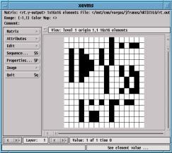
• XEVMS: matrix editor, enhanced version of the visualizer with capabilities for the cre-
ation and modification of images, as well as import/export features (Fig. 9).
file info
edition menus
image window
sequence browser
Fig.9: Input edition with the extended matrix viewer (XEVMS).
14SIRENA: A CAD Environment for Behavioral Modeling and Simulation of VLSI Cellular Neural Network Chips
III. CNN MODELLING WITH SIRENA
Development of the CNN paradigm (2) concerning aspects of the electronic implementa-
tion requires efficient CAD tools based on arbitrarily detailed descriptions of the network. Basic
algorithms and also low level physical effects must be representable. SIRENA makes use of an
especially developed high-level programming language DECEL. It is used to specify the com-
ponents --network constants and variables, and behavior of the cells --time evolution and com-
ponents bindings. This results in a model that can range from the pure algorithmic level to a
highly detailed description, with a vast number of non ideal characteristics accounting for pre-
dictable effects in electronic implementations (impedance coupling amongst input and output
nodes of the cells, undesired nonlinearities, parasitic elements effects, non-uniformity caused
by devices mismatch, etc.). SIRENA considers a CNN as a set of layers which evolve in an inde-
pendent but coordinated manner and interact in determined time instants by transferring some
variables value. Layer equations and variables are extracted from the DECEL description of the
CNN model. The whole network definition is stated by the declaration of all the layers consti-
tuting the complete CNN and a synchronization code. This outlines simulation timing schedule
and data interchange between layers in multi-layered networks and multi-network systems sim-
ulation. In other words, DECEL network definition begins at the bottom part of the hierarchy,
stating components and behavior of each elementary processor. Then, layer variables and equa-
tions come out from the collection of the components and behavior of each individual cell, and
finally, an assembly of synchronized (if required) layers conforms the top level --network defi-
nition. Let us describe some examples with different CNN implementations to illustrate the
modeling capabilities of SIRENA.
a) Chua and Yang original CNN model
The original model proposed by Chua and Yang [1] describes time evolution and neigh-
borhood coupling of each individual cell (c) within the grid domain (GD) in terms of a network
time-constant (τ), a radius of vicinity (r), feedback and control templates (a cd and b cd ) that
weight the influence of the neighbors’ input and output variables (u d and y d respectively) and an
offset term (d c) (Fig. 10). Cell state is the integral of a sum of weighted contributions from the
coupled neighboring processors, an offset term and a losses term, and cell output is a sigmoidal
non-linear function of the state, as expressed by the following equations:
dx c
τ -------- = – x c + ∑ { a dc y d + b dc u d } + d c ∀c ∈ GD (8)
dt d ∈ N (c)
r
–1 if x c < –1
c
y = f ( xc ) = xc if xc ≤ 1 (9)
1 if xc > 1
15SIRENA: A CAD Environment for Behavioral Modeling and Simulation of VLSI Cellular Neural Network Chips
(a dc /R)y d (a cc /R)y c (b cc /R)u c (b dc /R)u d f(xc)
1
-1 xc
+ + + 1
uc x c yc -1
R C c
d /R f(x ) −c
− −
Fig.10: CNN model originally proposed by Chua and Yang.
Some modified versions of this initial model introduce new features and algorithm extension,
like nonlinear or delay-type templates [13], or discrete-time emulations [14]. Other works report
a model oriented towards VLSI implementation [15].
DECEL definition of this ideal model (Fig. 11) begins with variable declaration. After
that, layer equations must be specified. This section is just a translation of the mathematical
statements (8) and (9) into DECEL syntax. Finally a network with one layer is declared:
chua.cs
layer chua
matrix u, x, y; //Input, state and output variables
layer
template a, b; //Feedback and control templates
components
bound bound_u, bound_y; //Boundary conditions declaration
scalar d; //Offset term
scalar tau; //Time constant
evolution layer
derivative(x) = (-x + a>SIRENA: A CAD Environment for Behavioral Modeling and Simulation of VLSI Cellular Neural Network Chips
This DECEL description of the CNN model is now compiled and the components and
behavior files are linked to the NSS for further utilization. As referred before, no information
about parameters value, nor even about network dimensions is contained inside the model
description. Instance values assignments, as well as network sizing, is done in different input
file, giving the model a large degree of generality. Any network of any size using any set of tem-
plates [16] for this CNN model can be simulated with this DECEL description, without recom-
piling the sources.
This ideal CNN model has been implemented in HSPICE (v. 95.1) using ideal elements
and piece-wise-linear voltage-controlled current sources, and also in SIRENA. Several simula-
tions have been run for different network sizes, ranging from 4 (arranged in a 2 × 2 matrix) to
1024 cells (32 × 32 matrix), in a Sun Microsystems SPARC Server 1000E with 4 CPUs and 512
Mb RAM. The employed templates performed Connected Component Detection of binary input
patterns [17]. The information generated by the system when running these simulation pro-
cesses under UNIX reports a certain advantage for SIRENA concerning the use of the system
resources. The following graph (Fig. 12) illustrates CPU time consumptions by SIRENA and
HSPICE. Fig. 13 shows the waveform plots of the cell state variable (xc) and the cell output vari-
able (yc) generated by HSPICE and SIRENA for the simulation of a 4 × 4 CNN based on Chua-
Yang model. R and C have been chosen to have a time constant of 1µs.
100
CPU time (seconds)
10
1
SIRENA
HSPICE
0
10 100 1000
number of cells (n)
Fig.12: Log-log graphs of the CPU time consumed by HSPICE (95.1) and SIRENA
simulations vs. the number of cells in the network.
17SIRENA: A CAD Environment for Behavioral Modeling and Simulation of VLSI Cellular Neural Network Chips
Input image Output pattern
Cell State Variable: X (volts)
SIRENA
HSPICE
Cell Output Variable: Y (volts)
SIRENA
HSPICE
Fig.13: Simulation waveforms of a 4 × 4 cells CNN for Connected Component Detection
using Chua-Yang original CNN model given by HSPICE (v.95.1) and SIRENA.
18SIRENA: A CAD Environment for Behavioral Modeling and Simulation of VLSI Cellular Neural Network Chips
b) OTA-based CNN implementation
In this section, a straight forward realization of a programmable CNN is going to be mod-
eled. This OTA based CNN [18] represents a direct mapping of the coupled differential equa-
tions defining the CNN dynamics onto some standard CMOS circuit primitives. In this
approach, an OTA block performs the nonlinear operation on the state variable (GmA in Fig. 14).
Multiplication of the input and output variables and the template elements is performed over the
output current of the OTA. This current has been replicated a number of times to implement the
whole set of template elements, a total of eighteen multipliers. As in [15], multiplication occurs
inside each cell and the properly weighted contribution is passed to the neighborhood. Because
of this, template elements should be reorganized to achieve the task for which they were
designed [3]. Currents, representing these neighbor contributions and the self-feedback compo-
nents, are added by wiring them together at the input node of each cell. Dynamic evolution of
every cell within the grid domain (GD) is described by:
dV x Vx
C x ij -----------ij = – --------ij + ∑ { Gm Akl ( V akl, V x kl ) + Gm Bkl ( V bkl, V ukl ) } + I bias (10)
dt R x ij k, l ∈ N
where GmA includes nonlinear operation and multiplication. To understand the way in which
this is accomplished let us have a look at the OTA-multiplier block implementation (Fig. 15).
To compute the currents through transistors Mn1 and Mn2, which operate as an input differential
pair, we have:
I B = I Mn1 + I Mn2 and β n V in = I Mn1 – I Mn2 (11)
from where it can be derived
I
IB if V in > ----B-
βn
I 2I I
I Mn1 = ----B- + β n V in -------B- – V 2in if V in ≤ ----B- (12)
2 βn βn
I
0 if V in < – ----B-
βn
and:
I
0 if V in > ----B-
βn
I 2I I
I Mn2 = ----B- – β n V in -------B- – V 2in if V in ≤ ----B- (13)
2 βn βn
I
IB if V in < – ----B-
βn
19SIRENA: A CAD Environment for Behavioral Modeling and Simulation of VLSI Cellular Neural Network Chips
ia00
from the neighbors
Vx f+(Vx)
Va00
GmA
f-(Vx)
Ibias Cx Rx
ia22
Va11 Va22 to the neighbors
ib00
f+(Vu)
Vb00
Vu
GmB
f-(Vu)
ib22
Vb11 Vb22
Fig.14: OTA-based CNN implementation conceptual schematics.
VDD
Mpm1 Mpm3
Mpm2 Mpm4
Vaij
+ Mn1 Mn2
Mp3 Mp4 Mp5 Mp6
Vin
− IB
io
Mnm1 Mnm2
VSS
Fig.15: CMOS realization of the OTA-multiplier block.
For the p-channel differential pairs we have, approximating by the first order term of a Taylor
20SIRENA: A CAD Environment for Behavioral Modeling and Simulation of VLSI Cellular Neural Network Chips
expansion, and within the linear range of operation Va ij ≤ I Mn ⁄ β p :
1, 2
I Mn I Mn
I Mp3 = ----------2 + 2β p I Mn2 Va ij I Mp5 = ----------1 – 2β p I Mn1 Va ij
2 2
and (14)
I Mn I Mn
I Mp4 = ----------2 – 2β p I Mn2 Va ij I Mp6 = ----------1 + 2β p I Mn1 Va ij
2 2
and therefore, the output current is given by:
I out ij = ( I Mp6 – I Mp5 ) – ( I Mp3 – I Mp4 ) = 2β p Va ij ( I Mn1 – I Mn2 ) (15)
Finally, using (11), (12) and (13), the output current of one of the multipliers can be
approximated as a piece-wise-linear function of the state variable:
I
2β p I B Va ij if V in > ----B-
βn
I
I out ij ≅ 2β p β Va ij V in if V in ≤ ----B- (16)
n βn
I
– 2β p I B Va ij if V in < – ----B-
βn
where the saturation limits are set to a value that becomes the normalizing factor for equation
(10) in order to represent the evolution of a CNN. Template elements have to be redesigned
because of this equation scaling [19]. Modelling of this specific implementation of a CNN
within SIRENA environment (Fig. 16 shows file ota.cs) includes the formal declaration of the
variables and CMOS parameters, relations between these variables, and the evolution section
with the differential equation.The model description ends with the network definition.
A comparison between HSPICE (v. 96) output and SIRENA results can be made in order
to validate this software implementation of the circuit. As before, templates for connected com-
ponent detection are employed. Table 1 shows the values assigned to each variable and param-
eter, extracted from HSPICE models of the CMOS devices and the analysis of the circuits
implementing the algorithm.
Level 3 models for the MOS devices have been used for HSPICE simulation. Using the
graphical user interface [20] the waveforms of the state variables of the CNN array can be gen-
erated and observed. Also, with the help of one of its format conversion tools, a plot of the out-
put of both simulators can be displayed with HSPICE graphic interface (GSI) for a comparison
(Fig. 15). Once again, reliability of this tool is stated by the similarity of the results obtained by
the two different simulators. CPU time and memory consumption figures give some advantage
to SIRENA when compared with HSPICE. In this case, for a 4 × 4 cells CNN simulation in a
SPARC Station 10/51 with 32 MB RAM, SIRENA needs 924kB RAM and 61.5 CPU seconds
compared to the 7452kB and 279.8 CPU seconds required by HSPICE.
21SIRENA: A CAD Environment for Behavioral Modeling and Simulation of VLSI Cellular Neural Network Chips
ota.cs
layer layer_otasc
matrix vx; //State variable (voltage)
matrix vu; // Input variable (voltage)
matrix i1x,i2x; //Differential pair currents
matrix i1u,i2u; //Differential pair currents
matrix i3a00,i4a00,i5a00,i6a00; //Multipliers currents
matrix i3b22,i4b22,i5b22,i6b22; //Multipliers currents
matrix iin; // Cell input node current
matrix io00x,io01x,io02x; //Output currents
layer
matrix io20u,io21u,io22u; //Output currents components
matrix ibias; // Bias term current declaration
matrix iout; //Output current
matrix b3a00,b4a00; //Multipliers parameters
matrix b3b22,b4b22; //Multipliers parameters
matrix ibi1,ibi2; // Bias term currents
template p00,p01,p02; //Evaluation of the neighborhood
template p10,p11,p12; //Evaluation of the neighborhood
template p20,p21,p22; //Evaluation of the neighborhood
boundary ic00x,ic01x,ic02x; //Boundary cells current
boundary ic20u,ic21u,ic22u; //Boundary cells current
scalar va00,va01,va02; // template voltages
scalar vb20,vb21,vb22; // template voltages
scalar vbias; // Bias term voltage
scalar cx,rx; // State capacitor & Loss Resistor
evolution
//Input Diff pair currents
i1x = [ vx >= sqrt(ibx/b1x) : ibx |vx = sqrt(ibu/b1u) : 0 |vu = sqrt(i2x/b3a00) : i2x |va00 = sqrt(i2u/b3b22) : i2u |vb22 = sqrt(i2u/b3b22) : 0 |vb22 = sqrt(i1u/b4b22) : i1u |vb22 = sqrt(i1u/b4b22) : 0 |vb22SIRENA: A CAD Environment for Behavioral Modeling and Simulation of VLSI Cellular Neural Network Chips
Input Output
Cell State Variable: Vx (volts)
SIRENA
HSPICE
Fig.17: Waveforms of state variables of an OTA-based 4 × 4 CNN performing Connected
Component Detection, simulated by HSPICE and SIRENA.
An extended version of this model could be employed for Montecarlo analysis of the cir-
23SIRENA: A CAD Environment for Behavioral Modeling and Simulation of VLSI Cellular Neural Network Chips
Variable, Parameter Name Value Units
Input and initial state (max) vx, vu 0.50 volts
Input and initial state (min) vx, vu -0.50 volts
Diff. pairs bias currents ibx, ibu 5.0 × 10⁻⁶ amps
NMOS transconductance b1x,...,b2u 240 × 10-6 A/V2
PMOS transconductance b3a00,...,b6b22 60 × 10-6 A/V2
Template elements (unity) va00,...,vb22 0.3 volts
Bias term voltage(unity) vbias 0.3 volts
Boundary currents (unity) ic00x,...,ic22u 3.0 × 10⁻⁶ amps
State variable capacitor cx 5.0 × 10⁻¹² farads
Losses resistor rx 5.0 × 10⁴ ohms
Table 1: OTA-based CNN model parameters.
cuit. This will be very useful to evaluate the implementation possibilities for a particular pro-
cess. Actual tolerance and parameter deviation can be specified and their influence studied with
the help of the statistical analysis capabilities of the environment.To take into account device
mismatches, some extra variables must be included in the OTA-based model. In addition, the
simplifications made to derive differential-pair currents (based on matched transistors) can not
be assumed. As a consequence, the description of a simple differential pair becomes more com-
plicated. As a starting point, let us consider that there are slight differences between electrical
parameters (transconductance and threshold voltage) of the two ideally matched transistors of a
differential pair:
∆β ∆V Tn
β n1 = β n + ---------n V Tn1 = V Tn + ------------
-
2 2
and (17)
∆β ∆V Tn
β n2 = β n – ---------n V Tn2 = V Tn – ------------
-
2 2
The currents flowing through each of the two devices, given before by (12) and (13), are now
expressed by:
24SIRENA: A CAD Environment for Behavioral Modeling and Simulation of VLSI Cellular Neural Network Chips
IMn1 = ((2βn + ∆βn)(-2βn∆βn∆VTn2 + ∆βn2∆VTn2 + 4βnIB + 4βn∆βn∆VTnVin−
2∆βn2∆VTnVin - 2βn∆βnVin2 + ∆βn2Vin2 + (2βn − ∆βn )(Vin− ∆VTn)
(18)
sqrt(- 4βn2∆VTn2 + ∆βn2∆VTn2 +8βnIB+ 8βn2∆VTnVin− 2∆βn2∆VTnVin
- 4βn2Vin2 + ∆βn2Vin2)))/16βn2
IMn2 = ((2βn - ∆βn)(2βn∆βn∆VTn2 + ∆βn2∆VTn2 + 4βnIB + 4βn∆βn∆VTnVin−
2∆βn2∆VTnVin - 2βn∆βnVin2 + ∆βn2Vin2 + (2βn + ∆βn )(Vin− ∆VTn)
(19)
sqrt(- 4βn2∆VTn2 + ∆βn2∆VTn2 +8βnIB+ 8βn2∆VTnVin− 2∆βn2∆VTnVin
- 4βn2Vin2 + ∆βn2Vin2)))/16βn2
c) A current-mode CNN model based on a hardware realization
In order to deepen inside SIRENA macromodeling capabilities, let us consider now the
current mode implementation [15] of a CNN based on the exhaustive use of current mirrors, and
designed to perform Connected Component Detection [17] of binary input patterns. Templates
for this operation have the following values:
0 0 0 0 0 0
A = 1 2 –1 B = 0 0 0 d = 0 (20)
0 0 0 0 0 0
This specific-application CNN is rather simple, having null control template and offset term,
and only two neighbors connected. Still, it will be useful to illustrate the capabilities of
SIRENA. Besides, this circuit has been successfully designed, integrated, proven and reported
[21].
Let us consider the schematic of the basic processor depicted in Fig. 18. First, state vari-
ables of basic cells must be appointed, and their evolution laws must be established. We have
chosen the voltages across capacitors Cx, Cyp and Cyn to be our state variables, namely: x, yp and
yn. These two latter are the output variables of the cell, limited versions of the cell state x, each
with different sign. In these conditions, time evolution of the three state variables is described
(with the help of some auxiliary currents that will be defined later) by the following set of equa-
tions:
25SIRENA: A CAD Environment for Behavioral Modeling and Simulation of VLSI Cellular Neural Network Chips
icpx
VG
icpyp icpyp icpyn icpyn
icx icyp icyn
icn2yp icn2yn
icn1yp icn1yn +
icnx
+ +
yn
x yp
−
Cx Cyp Cyn
− −
2icpc icpl icpr
VG
x2
2icnc icnr
ypl icnl ynr
x x2
Fig.18: Schematic diagram of a current-mode CNN cell for Connected Component
Detection based on bias-shifted current mirrors.
dx i cx
----- = -----
-
dt Cx
dy p i cyp
-------- = -------- (21)
dt C yp
dy n i cyn
-------- = --------
dt C yn
Now, current icx is the sum of a feedback term, double of the current generated by cell state vari-
able, and the neighbors contribution with the sign commanded by the feedback template, apart
from the current injected by the current mirror supporting the state capacitor. Each current con-
tribution towards this node has a positive component, due to the current sources implemented
with PMOS transistors, and a negative term dragged by the n-channel devices,
i cx = 2 ( i cpc – i cnc ) + ( i cpl – i cnl ) + ( i cpr – i cnr ) + ( i cpx – i cnx ) (22)
Currents flowing towards the other two state capacitors are computed in a similar manner:
i cyp = 2i cpyp – i cn1yp – i cn2yp (23)
26SIRENA: A CAD Environment for Behavioral Modeling and Simulation of VLSI Cellular Neural Network Chips
i cyp = 2i cpyp – i cn1yp – i cn2yp (24)
Finally, each term in (22), (23) and (24) is obtained from level-one Schichman-Hodges MOS
transistor equations for the drain-to-source current, detailed here for a clearer exposition of the
DECEL description of this current-mode CNN model. For NMOS transistors:
0 if V gs < V Tn
2
V ds
k s ( V – V )V – -------- if V ds ≤ V gs – V Tn
I ds = n n gs Tn ds 2 (25)
k
----n- s n ( V gs – V Tn ) 2 if V ds > V gs – V Tn
2
while for PMOS devices:
0 if V sg > V DD – V Tp
V sd 2
( V sg – V Tp )V sd – -------- V sd ≤ V sg – V Tp
I sd = k ps p 2
- if (26)
k
----p- s p ( V sg – V Tp ) 2 if V sd > V sg – V Tp
2
Once the state variables and equations are stated, a DECEL description of the model can
be made (Fig. 19). Let us go through cm.es file. Within layer components declaration, state vari-
ables are defined as matrices. Neighbors’ output matrices are defined also for convenience.
After that, auxiliary currents used to evaluate the contributions to the time derivatives (21) of
the state variables are stated. It is necessary to have the information about neighbors output vari-
able within each cell to compute the contributions icpl, icpr, icnl and icnr to the current flowing
through node x. Two templates are declared for this purpose (weights of the connections can be
included here or left to further description within layer equations statement). Finally, boundary
conditions and several design and technological parameters are declared, namely the power sup-
ply and bias voltages, transistor aspect ratios, transconductance parameters and threshold volt-
ages, and state capacitors.
Layer equations are depicted next. At the beginning of this section, output variables of the
neighbors are assigned to cell variables yl and yr. After that, auxiliary currents are calculated
based on the transistor model described by (25) and (26), concluding with DECEL statements
equivalent to equations (22), (23) and (24). This evolution section ends with the time evolution
laws of the state variables (21). The last part of the model description is the network definition,
and once again this is a one-layer CNN.
Table 2 shows the values assigned to each variable and parameter, extracted from HSPICE
models of the CMOS devices and circuit analysis.
27SIRENA: A CAD Environment for Behavioral Modeling and Simulation of VLSI Cellular Neural Network Chips
cm.cs
layer layer_cm
matrix x, yp, yn ; //State Variables
matrix yl, yr; //Neighborhood State Variables
matrix icx, icyp, icyn; //Auxiliary currents
layer
matrix icn1yn,icn2yn,icn1yp2, icn1yn2;
components
declaration
template ayl,ayr; //Template for neighbor state evaluation
boundary bound_yp,bound_yn; //Boundary conditions (yp, yn)
scalar vdd, vg; //Power Supply and Bias Voltage
scalar sn,sp; //MOS Trans. Geometric aspect ratio
scalar kp,kn,vtp,vtn; //Techn. Parameters
scalar cx, cyp, cyn; //State Capacitors
evolution
yl= ayl> (yl-vtn) : (kn/2)*sn*(yl-vtn)*(yl-vtn) |
kn*sn*((yl-vtn)*x -x*x/2) ];
icnl= [ yl > vtn : icnl2 | 0 ];
icpr=icpl ;
icnr2= [ x > (yr-vtn) : (kn/2)*sn*(yr-vtn)*(yr-vtn) |
kn*sn*((yr-vtn)*x -x*x/2) ];
icnr= [ yr > vtn : icnr2 | 0 ];
icpc=2*icpl ;
layer
equations
icnc2= [ x > (yp-vtn) : kn*sn*(yp-vtn)*(yp-vtn) |
2*kn*sn*((yp-vtn)*x -x*x/2) ];
icnc= [ yp > vtn : icnc2 | 0 ];
icpx= icpl;
icnx= [ x < vtn : 0 | (kn/2)*sn*(x-vtn)*(x-vtn) ];
icpyp= [ yp < vg+vtp : (kp*sp/2)*(vdd-vg-vtp)*(vdd-vg-vtp) |
kp*sp*((vdd-vg-vtp)*(vdd-yp)-(vdd-yp)*(vdd-yp)/2) ];
icn1yp2= [ yp > (x-vtn) : (kn/2)*sn*(x-vtn)*(x-vtn) |
kn*sn*((x-vtn)*yp -yp*yp/2) ];
icn1yp= [ x > vtn : icn1yp2 | 0 ];
icn2yp= [ yp < vtn : 0 | (kn/2)*sn*(yp-vtn)*(yp-vtn) ];
icyp= 2*icpyp-icn1yp-icn2yp;
icpyn= [ yn < vg+vtp : (kp*sp/2)*(vdd-vg-vtp)*(vdd-vg-vtp) |
kp*sp*((vdd-vg-vtp)*(vdd-yn)-(vdd-yn)*(vdd-yn)/2) ];
icn1yn2= [ yn > (yp-vtn) : (kn/2)*sn*(yp-vtn)*(yp-vtn) |
kn*sn*((yp-vtn)*yn -yn*yn/2) ];
icn1yn= [ yp > vtn : icn1yn2 | 0 ];
icn2yn= [ yn < vtn : 0 | (kn/2)*sn*(yn-vtn)*(yn-vtn) ];
icyn= 2*icpyn-icn1yn-icn2yn;
derivative(x)= icx/cx;
derivative(yp)= icyp/cyp;
derivative(yn)= icyn/cyn;
network
network
sublayer layer_cm cm; definition
end
Fig.19: DECEL description of the current-mode CNN model
28SIRENA: A CAD Environment for Behavioral Modeling and Simulation of VLSI Cellular Neural Network Chips
Variable, Parameter Name Value Units
Initial state (max.) x, yp, yn 0.98 volts
Initial state (min.) x, yp, yn 0.70 volts
Power Supply voltage vdd 5.0 volts
Bias voltage vg 3.6 volts
NMOS transconductance kn 45 × 10-6 A/V2
PMOS transconductance kp 15.4 × 10⁻⁶ A/V2
NMOS threshold voltage vtn 0.60 volts
PMOS threshold voltage vtp 0.98 volts
State capacitor (I) cx 0.450 × 10⁻¹² farads
State capacitor (II) cyp 0.112 × 10⁻¹² farads
State capacitor (III) cyn 0.042 × 10⁻¹² farads
Positive boundary condition bound_yp 0.98 volts
Positive boundary condition bound_yn 0.70 volts
Losses resistor rx 5.0 × 10⁴ ohms
Table 2: Current-mode CNN model parameters.
Fig. 20 shows the waveform plots of the state variable x and the output variable yp of every
cell in a 4 × 4 current-mode CNN obtained from HSPICE (using level-two models for MOS)
and from SIRENA using the macromodel described above. Notice that sign of yp is reversed
from that of the state variable due to the current inversion imposed by mirroring. Time scale of
these graphs, in the range of tenths of microseconds, begin at 100ns because of network initial-
ization. Similarity between each of the sixteen pairs of curves gives an idea of the accuracy of
the macromodel employed in SIRENA. A higher degree of precision could be reached with the
inclusion of second order effects like mobility degradation, non-linear gate capacitance, chan-
nel-length modulation, etc.
As with previous examples, several HSPICE and SIRENA simulations of different-size
networks have been realized with the same machine (SPARC Server 1000E). CPU time plots
versus network size (Fig. 21) shows a considerable advantage for SIRENA, reaching two orders
of magnitude for large networks. The larger efficiency of this environment, within the scope for
which it was developed, is therefore clear.
d) A Discrete-Time Hard-nonlinearity non-linear CNN model
Finally, in order to illustrate the broad variety of network types that can be described in
29SIRENA: A CAD Environment for Behavioral Modeling and Simulation of VLSI Cellular Neural Network Chips
Input image Output pattern
Cell State Variable: X (volts)
SIRENA
HSPICE
Cell Output Variable: Yp (volts)
SIRENA
HSPICE
Fig.20: Simulation waveforms of a 4 × 4 cells Current-Mode CNN for Con-
nected Component Detection obtained from HSPICE and SIRENA.
30SIRENA: A CAD Environment for Behavioral Modeling and Simulation of VLSI Cellular Neural Network Chips
10000
1000
CPU time (seconds)
100
10
SIRENA
HSPICE
1
10 100 1000
number of cells (n)
Fig.21: Log-log graphs of CPU times consumed by HSPICE (95.1) and SIRENA vs. number of cells in the
network.
DECEL language, let us consider the case of a discrete-time CNN chip to perform the Radon
Transform operation [22]. Some peculiar properties of this algorithm include the hard-limitation
of the cell output variable and the use of non-linear template elements (which depend of the cell
state). The operation consists on computing the integral of intensity values along each row of
the network. For binary images, this results in a histogram of the input pattern. The discrete-
time evolution of the network is now described by a system of finite-differences equations,
∑
c c c d
x (n + 1) = a d [ y ( n ) ]y ( n ) ∀c ∈ GD (27)
d ∈ N r(c)
where the non-linear feedback template is described by
0 0 0
1 – yc 1 + yc
A ( y c ) = ------------- ∀c ∈ GD (28)
- 0 --------------
2 2
0 0 0
and where the output variable is obtained through a hard-limiting non-linear function:
c
c c 1 if x >0
y (n) = f [ x (n)] = ∀c ∈ GD (29)
–1 if
c
x ≤0
Several differences can be observed between this network-model and those reported
before. First of all, this is a discrete-time CNN. This forces the definition of a set of variables
31SIRENA: A CAD Environment for Behavioral Modeling and Simulation of VLSI Cellular Neural Network Chips
within the DECEL description of the model (file dt.cs in Fig. 22) for evaluate convergence eval-
uation during the simulation process. Feedback-template dependence on the cell output must be
included in the evolution law of the model, and therefore the connection operator must store
neighbors output variables into separate matrices. The last part of the model description is the
network definition.
dt.cs
layer layer_rt
matrix x,y; //Input and output variables
matrix y1,y2; //Neighbours output variables
template a1,a2; //Neighbours evaluation templates
layer
boundary bound_y; //Boundary conditions components
declaration
sets
(states x,y); //Evaluation of convergence
end
evolution
y1= a1>You can also read