Contribution of personal weather stations to the observation of deep-convection features near the ground
←
→
Page content transcription
If your browser does not render page correctly, please read the page content below

Nat. Hazards Earth Syst. Sci., 20, 299–322, 2020
https://doi.org/10.5194/nhess-20-299-2020
© Author(s) 2020. This work is distributed under
the Creative Commons Attribution 4.0 License.

Contribution of personal weather stations to the observation
of deep-convection features near the ground
Marc Mandement and Olivier Caumont
CNRM, Université de Toulouse, Météo-France, CNRS, Toulouse, France

Correspondence: Marc Mandement (marc.mandement@meteo.fr)

Received: 11 July 2019 – Discussion started: 17 July 2019
Revised: 2 December 2019 – Accepted: 12 December 2019 – Published: 24 January 2020

Abstract. The lack of observations near the surface is often     panying most of the storms were observed sooner and at a
cited as a limiting factor in the observation and prediction     finer resolution in SPWS analyses than in SWS analyses. The
of deep convection. Recently, networks of personal weather       virtual potential temperature was spatialized at an unprece-
stations (PWSs) measuring pressure, temperature and humid-       dented spatial resolution. This provided the opportunity for
ity in near-real time have been rapidly developing. Even if      observing cold-pool propagation and secondary convective
they suffer from quality issues, their high temporal resolu-     initiation over areas with high virtual potential temperatures,
tion and their higher spatial density than standard weather      i.e. favourable locations for near-surface parcel lifting.
station (SWS) networks have aroused interest in using them
to observe deep convection. In this study, the PWS contribu-
tion to the observation of deep-convection features near the
ground is evaluated. Four cases of deep convection in 2018       1   Introduction
over France were considered using data from Netatmo, a
PWS manufacturer. A fully automatic PWS processing algo-         The increasing number of connected objects – i.e. with Inter-
rithm, including PWS quality control, was developed. After       net access – which carry meteorological sensors has raised
processing, the mean number of observations available in-        the interest of scientists because they are a supplementary
creased by a factor of 134 in mean sea level pressure (MSLP),    means of observing the atmosphere. Several publications
of 11 in temperature and of 14 in relative humidity over         emphasize the high potential of these sensors for the fine-
the areas of study. Near-surface SWS analyses and analy-         scale observation of atmospheric phenomena, complemen-
ses comprising standard and personal weather stations (SP-       tary to traditional sources, given the unprecedented spatio-
WSs) were built. The usefulness of crowdsourced data was         temporal resolution of the networks constituted by these sen-
proven both objectively and subjectively for deep-convection     sors (Muller et al., 2015; Chapman et al., 2017). These new
observation. Objective validations of SWS and SPWS anal-         observations come from smartphones (Overeem et al., 2013;
yses by leave-one-out cross validation (LOOCV) were per-         Mass and Madaus, 2014; McNicholas and Mass, 2018a),
formed using SWSs as the validation dataset. Over the four       connected vehicles (Mahoney and O’Sullivan, 2013) or per-
cases, LOOCV root-mean-square errors (RMSEs) decreased           sonal weather stations (PWSs hereafter, also called citizen
for all parameters in SPWS analyses compared to SWS anal-        weather stations; Bell et al., 2013), for example. All these
yses. RMSEs decreased by 73 % to 77 % in MSLP, 12 % to           studies underline the potential gains in the fine-scale descrip-
23 % in temperature and 17 % to 21 % in relative humidity.       tion of the atmosphere near the ground.
Subjectively, fine-scale structures showed up in SPWS anal-         Among all meteorological processes, deep convection in-
yses, while being partly, or not at all, visible in SWS obser-   duces the sharpest variations in pressure, temperature, hu-
vations only. MSLP jumps accompanying squall lines or in-        midity, wind and rain near the ground. Recognition of deep-
dividual cells were observed as well as wake lows at the rear    convection surface features such as low-level convergence
of these lines. Temperature drops and humidity rises accom-      boundaries (Wilson and Schreiber, 1986; Wakimoto and
                                                                 Murphey, 2010), pressure, temperature and humidity fea-

Published by Copernicus Publications on behalf of the European Geosciences Union.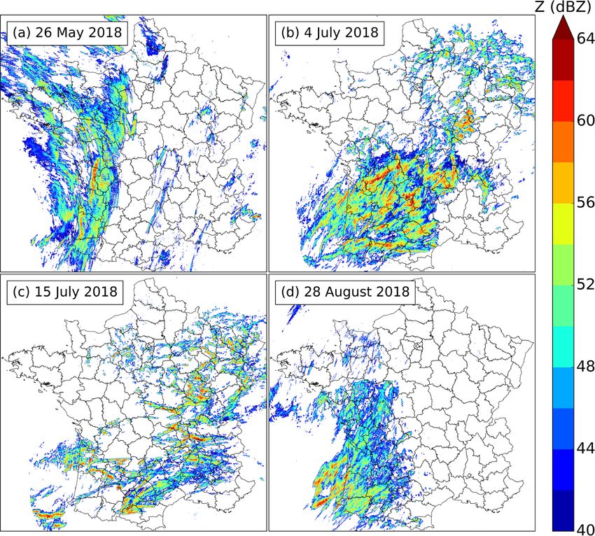
300              M. Mandement and O. Caumont: Contribution of PWSs to the observation of deep-convection features

tures prior to convection (Madaus and Hakim, 2016), as well        ics well according to a simulation study under ideal mea-
as tracking their temporal evolution, is deemed crucial for        surements conditions (de Vos et al., 2018). Subsequently, a
thunderstorm forecasting (Sanders and Doswell, 1995). The          real-time quality-control algorithm of rain gauges produced
prediction of convective initiation location and timing, as        by Netatmo, a PWS manufacturer, was developed in order
well as its evolution, still remain a challenging question.        to complement traditional networks for operational rainfall
Several studies agree that there is a lack of observations at      monitoring (de Vos et al., 2019). Recently, Clark et al. (2018)
the surface, which limits the quality of analyses at the con-      showed the benefit of PWS data in the life-cycle observation
vective scale and in turn limits good forecasts of convec-         of a hailstorm that crossed the UK in 2015. The supplemen-
tive events (Stensrud and Fritsch, 1994; Fowle and Roeb-           tary data in temperature, pressure, wind speed given by the
ber, 2003; Snook et al., 2015; Sobash and Stensrud, 2015).         PWSs associated with the UK Met Office network revealed
Observational studies highlight a need for additional high-        fine-scale structures corresponding to conceptual models of
resolution observations (Adams-Selin and Johnson, 2010;            severe thunderstorms. However, the quality-control proce-
Clark, 2011) because deep convection is often associated           dures were not fully automatic, and a manual check of each
with small-scale parameter variations. Additionally, there is      dataset had to be performed.
a need for validating high-resolution numerical models and            The goal of the present study is to evaluate the contribu-
verifying their accuracy of deep-convection modelling.             tion of PWSs to the existing standard weather station (SWS)
   These statements motivated experiments in several fields        network in the observation of deep-convection processes at
of meteorology. They have been led using denser observa-           midlatitudes over France. A fully automatic PWS processing
tional networks near the ground for the study of a particular      algorithm based on comparisons with SWSs was developed.
storm, for urban climate studies or for hydrological appli-        The features near the ground of isolated storms, multicellu-
cations. Several assimilation experiments of denser weather        lar systems or supercell storms are observed, extending the
station networks or observations made with connected ob-           work of Clark et al. (2018), which focused on a sole supercell
jects have also already been performed. Madaus et al. (2014)       storm. Observed features of processes responsible for their
performed an hourly assimilation of dense pressure observa-        formation or generated by these systems such as cold pools,
tions from mesonets. Results showed an increase in short-          gust fronts and sea breeze effects are studied. In order to do
term forecast accuracy for temperature, wind and pressure          so, mean sea level pressure (MSLP), temperature and humid-
near mesoscale phenomena. It was shown that 5 min assimi-          ity gridded analyses including PWSs are built. The additional
lation of mesonet data (Sobash and Stensrud, 2015) or non-         value of these weather stations is objectively evaluated by
conventional data (Gasperoni et al., 2018), mostly thermody-       comparison with reference gridded analyses made only with
namic observations, improved forecasts of convection initia-       SWSs. First, in Sect. 2 this study describes interesting con-
tion.                                                              vective cases of the spring and summer of 2018 over France.
   Regarding connected objects, several recent data assim-         In Sect. 3, a presentation of the different weather station
ilation experiments focused on smartphone observations             networks used in the study is made. The processing includ-
(Madaus and Mass, 2017; McNicholas and Mass, 2018b;                ing a quality control of PWSs measurements is detailed in
Hintz et al., 2019). Assimilating smartphone pressure mea-         Sect. 4, followed by the validation performed against SWSs
surements led to some improvements in analyses and short-          in Sect. 5. Then, a focus on some features observed during
term forecasts of surface variables compared to experiments        the different convective cases is made in Sect. 6 to evidence
without assimilation of observations. Results shown were           the positive contribution of PWSs.
strongly sensitive to the quality-control techniques developed
in each study. This demonstrates that quantifying the uncer-
tainties associated to these observations, and establishing ro-    2   Overview of the cases
bust quality-control procedures, is crucial. In parallel, recent
                                                                   Four cases are chosen to evaluate the contribution of the
work has been done in the urban climate communities that
                                                                   PWS network to the observation of deep-convection features
examines phenomena at a city scale, benefiting from a high
                                                                   near the ground. The considered cases and the periods of
number of connected objects due to the high population den-
                                                                   time of the cases are indicated in Table 1. The casualties
sity in cities. Temperature measurements from PWSs have
                                                                   and damage listed in each case come from internal reports of
been used to visualize the urban heat island in several west-
                                                                   the French emergency management agency (Sécurité Civile),
ern European cities (Wolters and Brandsma, 2012; Chap-
                                                                   press releases from the prefectures, press releases from the
man et al., 2017; Meier et al., 2017; Napoly et al., 2018).
                                                                   French distribution grid operator (Enedis) and press archives
These studies showed that PWSs can provide robust esti-
                                                                   (France 3, Sud Ouest).
mates of temperature at a fine scale when measurements
are quality-controlled and spatially aggregated. For precip-
itation, de Vos et al. (2017) showed that dense PWS net-
works can be used for urban rainfall monitoring in Ams-
terdam and are able to capture small-scale rainfall dynam-

Nat. Hazards Earth Syst. Sci., 20, 299–322, 2020                            www.nat-hazards-earth-syst-sci.net/20/299/2020/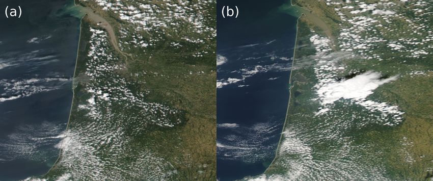
M. Mandement and O. Caumont: Contribution of PWSs to the observation of deep-convection features                                     301

Table 1. Periods of time of each case study.

                            Date               26 May 2018   4 July 2018    15 July 2018     28 August 2018
                            Start time (UTC)   06:55         05:55          00:15            12:55
                            End time (UTC)     23:55         21:55          23:55            23:55

2.1   26 May 2018: bow echo over the west of France

On 26 May 2018 a mid-level low at 500 hPa was located in
the Bay of Biscay (Fig. 1). This induced a moderate southerly
flux over France: the Bordeaux sounding at 23:00 UTC on
25 May observed a 11 m s−1 southerly wind at 500 hPa. Two
positive (cyclonic) upper-level potential vorticity anomalies
circulated during the day in the southerly flux observed near
the tropopause (Fig. 2a). At the surface, a shallow pressure
low around 1010 hPa in the bay headed north very slowly
during the day. Pressure gradients were weak all over the
western part of France. Over the south-west of France, the
air was mild and humid due to the convective activity that
occurred the day before and in the early hours of 26 May.
Indeed, a first mesoscale convective system (MCS) evolved
mainly on the Atlantic Ocean, its edges affecting the French
Atlantic coast from the Basque Country to Brittany be-
tween 25 May at 22:00 UTC and 26 May at 16:00 UTC. The
Bordeaux 25 May 23:00 UTC sounding, the closest avail-               Figure 1. Topographic map of metropolitan France. Domains stud-
able before the event, exhibited only 416 J kg−1 surface-            ied are drawn in red, and locations mentioned are indicated in black.
                                                                     Domain A corresponds to the 26 May case, domain B corresponds
based convective available potential energy (SBCAPE) and
                                                                     to the 28 August case, and domain C corresponds to the 4 and
strong 245 J kg−1 convective inhibition (CIN) because of the         15 July cases.
decrease in temperature near the surface due to the diur-
nal cycle. However it recorded a 1583 J kg−1 most-unstable
CAPE (MUCAPE) from the lifting of a 435 m a.g.l. (above                 The supercell produced damaging hail up to 4 cm in di-
ground level) air parcel (25 J kg−1 CIN for this parcel). This       ameter and rain up to 22 mm in 6 min in the centre of Bor-
shows the presence of unstable levels above the stable noc-          deaux. The bow echo produced mainly strong wind gusts up
turnal boundary layer. The sounding observed a moderate 0–           to 31 m s−1 : 13 SWSs recorded gusts higher than 25 m s−1 ,
6 km a.g.l. 16 m s−1 wind shear, and the hodograph exhibited         and 4 of them recorded gusts higher than 28 m s−1 (Fig. 4a).
a clockwise rotation of the winds in the 0–1 km a.g.l. layer,        The two systems resulted in one fatality, 1555 rescue opera-
resulting in a 69 m2 s−2 helicity.                                   tions and 15 000 homes being without power. This produced
   At the rear of the first MCS, thunderstorms formed in the         also local flash floods in Bordeaux and hail damage in the
north of Spain, west of the Pyrenees, between 06:00 and              Bordeaux vineyards.
08:00 UTC. These cells, advected by the mid-troposphere
southern flux, crossed the Pyrenees and headed north towards         2.2   4 July 2018: squall line over the south-west of
Bordeaux. A squall-line organization of the thunderstorms                  France
appeared at around 10:00 UTC. This MCS transitioned into a
bow echo at around 13:00 UTC according to radar reflectivi-          On 4 July 2018, a mid-level low at 500 hPa was located
ties and crossed the west of France, moving in a south–north         over the Atlantic Ocean and was extended by a trough
orientation from the Bordeaux region towards Normandy and            across the Iberian Peninsula. The trough moved west to-
Great Britain (Fig. 3a). The system was still active when it         wards France during the day, inducing a moderate south-
left the French territory at 23:00 UTC. The path followed by         westerly flux at the mid-level over the west of France: the
the bow echo can be seen west of France in Fig. 4a, marked           Bordeaux sounding observed a south-westerly 12 m s−1 wind
by the area of high-speed, diverging wind gusts. Also, to the        at 23:00 UTC on 3 July and south–south-westerly 16 m s−1
north of the MCS, a severe isolated thunderstorm, identi-            wind at 11:00 UTC on 4 July. An upper-level potential vor-
fied as a supercell in the radar imagery, developed at around        ticity anomaly circulated during the afternoon over France
10:30 UTC and merged with the MCS at around 15:00 UTC.               at the rear of the convective area and on the left side of a

www.nat-hazards-earth-syst-sci.net/20/299/2020/                                Nat. Hazards Earth Syst. Sci., 20, 299–322, 2020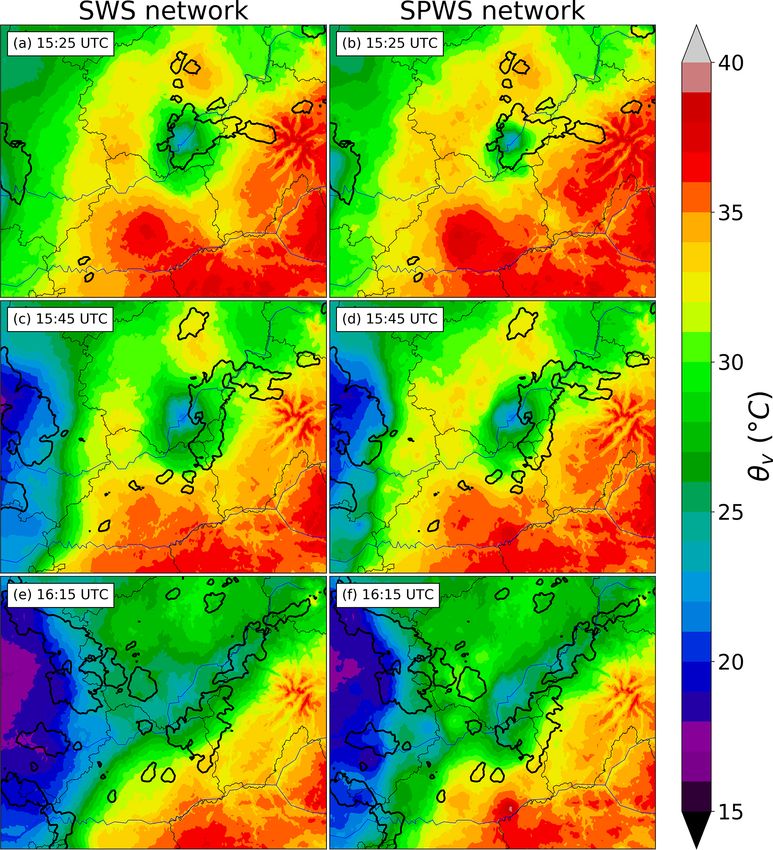
302               M. Mandement and O. Caumont: Contribution of PWSs to the observation of deep-convection features

Figure 2. Europe and North Atlantic graphical synoptic analysis charts (a) at 00:00 UTC on 26 May 2018, (b) at 12:00 UTC on 4 July 2018,
(c) at 12:00 UTC on 15 July 2018 and (d) at 12:00 UTC on 28 August 2018 (Santurette and Joly, 2002). MSLP isobars from ARPEGE model
6 h forecast of the T − 6 h run (T : time of the chart) are drawn at 5 hPa intervals. Surface fronts are shown by conventional symbols. Lows
are indicated by “D” and highs by “A” with the pressure tendency observed. PV stands for potential vorticity. Adapted from Météo-France
national forecast department.

jet stream branch (Fig. 2b). At the surface, a shallow low              hodograph, resulting in 0–3 km a.g.l. 79 m2 s−2 helicity. The
was located south-west of England, and pressure gradients               system generated peak wind gusts up to 34 m s−1 . A large
were weak all over France. Isolated thunderstorms affected              area was affected by strong wind gusts: more than 30 SWSs
the south-west of France on the night of 3 to 4 July. In the            recorded gust speeds higher than 25 m s−1 , and 11 of them
morning of 4 July, at around 09:00 UTC, numerous thunder-               recorded gusts higher than 28 m s−1 (Fig. 4b). Flash floods
storms developed in the north of Spain, over the Bay of Bis-            were observed, with rain rates up to 41.6 mm in 18 min. This
cay and in the south-west of France. They aggregated in sev-            resulted in one fatality, six injuries, 2500 rescue operations
eral multicellular systems. Embedded in one of these systems            and 185 000 homes being without power. Tennis-ball-sized
over the south-west of France, one of the storms exhibited              hail (> 6 cm in diameter) was reported: in a village named
supercellular characteristics in the radar imagery. At around           Saint-Sornin, 800 houses were seriously damaged. This hail
12:00 UTC, another multicellular system formed north of                 was caused by the storm identified as a supercell, in which
Spain, strengthened over the Atlantic Ocean and transitioned            reflectivities up to 70 dBZ were measured by radar.
into a squall line. The squall line headed north-east while
isolated storms formed in its southern part. It finally merged          2.3    15 July 2018: isolated storms over the south-west of
with other storms at around 17:00 UTC, and the isolated cells                  France
south of it merged in clusters, most of them evolving along
with a strong MSLP gradient area (Fig. 3b). The sounding                On 15 July 2018, a mid-level trough at 500 hPa circulated
of Bordeaux at 11:00 UTC, before the arrival of the squall              from Portugal towards the west of France, inducing west–
line at 14:00 UTC, exhibited large 2155 J kg−1 SBCAPE,                  south-westerly winds in mid-troposphere. An upper-level po-
weak 12 J kg−1 CIN and a moderate clockwise-rotating wind               tential vorticity anomaly circulated over the south-west of

Nat. Hazards Earth Syst. Sci., 20, 299–322, 2020                                  www.nat-hazards-earth-syst-sci.net/20/299/2020/
M. Mandement and O. Caumont: Contribution of PWSs to the observation of deep-convection features                                      303

Figure 3. Maximum base reflectivity for each case study: (a) 26 May 2018, (b) 4 July 2018, (c) 15 July 2018 and (d) 28 August 2018.

Figure 4. Peak wind gusts measured over metropolitan France (a) on 26 May 2018, (b) on 4 July 2018 and (c) on 28 August 2018. Adapted
from Météo-France climatological service.

France during the afternoon in a north-eastward direction             30 ◦ C with clear sky and the inland area where temperatures
(Fig. 2c). At the surface, pressure gradients were weak over          reached 32 to 33.5 ◦ C and cumulus clouds were developing.
France. The sounding of Bordeaux at 11:00 UTC exhibited               Surface observations and satellite images showed the wind
a SBCAPE of 1790 J kg−1 and a CIN of 0 J kg−1 , showing               convergence due to the breeze moving eastwards between
ideal conditions for the development of surface-based con-            12:30 and 13:45 UTC. At around 13:10 UTC, towering cu-
vection. A sea breeze established near the Atlantic shore             muli turned into cumulonimbi at the south-east of Arcachon
,and its effects on cloud coverage were visible on satel-             Bay (Fig. 5b), where SWSs measured the strongest temper-
lite images at 12:39 UTC (Fig. 5a). A frontier appeared be-           ature gradient with a 5 ◦ C difference in a 40 km distance.
tween the coastal band where temperatures reached 27 to               The initiation happened along the wind convergence line.

www.nat-hazards-earth-syst-sci.net/20/299/2020/                                  Nat. Hazards Earth Syst. Sci., 20, 299–322, 2020
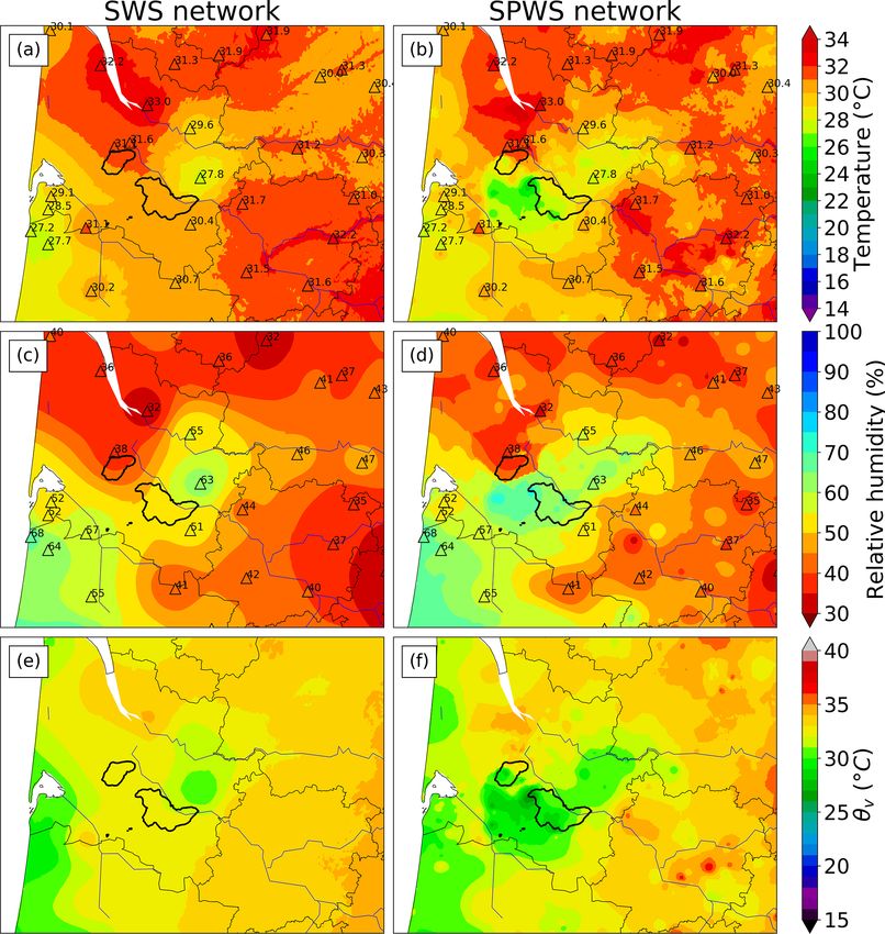
304              M. Mandement and O. Caumont: Contribution of PWSs to the observation of deep-convection features

Figure 5. Visible satellite images of convective initiation due to sea breeze convergence on 15 July 2018 taken by (a) Suomi NPP–VIIRS at
12:39 UTC and (b) Aqua MODIS at 13:43 UTC. Images from NASA Worldview.

The first cell triggered secondary cell development west and           by lightning. Hail up to 8 mm in diameter was reported near
north of it. Two main cells split and evolved in different di-         the coast.
rections: the first one headed north–north-east and the other
one headed east (Fig. 3c). The cell evolving north–north-east
caused high wind gusts up to 34 m s−1 at the Bordeaux air-             3     Datasets
port at 15:05 UTC, and the temperature dropped by 15.5 ◦ C
in 23 min. Hail diameters of up to 3 cm were observed in the           Two main surface networks are used: automatic SWSs taken
Bordeaux region under the thunderstorm. This event caused              as a reference and Netatmo PWSs. To associate surface fea-
84 rescue operations and happened in the context of public             tures to the thunderstorm activity, storms are mainly tracked
gatherings due to the football World Cup Final.                        with the French radar network.

                                                                       3.1    SWS network
2.4   28 August 2018: two squall lines over the west of
      France                                                           SWSs are all automatic Météo-France operational weather
                                                                       stations sampling atmospheric parameters at a time step of
                                                                       1 min. These weather stations have been installed, main-
On 28 August 2018, a mid-level trough at 500 hPa con-                  tained and quality-controlled by Météo-France. The require-
cerned the west of France and moved slightly eastwards dur-            ments in terms of accuracy for Météo-France weather sta-
ing the day, resulting in a south–south-easterly flux. At the          tions are ±0.5 ◦ C in temperature and ±6 % in relative hu-
surface a low centred north of the Iberian Peninsula deep-             midity (Tardieu and Leroy, 2003). They are taken as a ref-
ened during the day (Fig. 2d), helped by a potential vortic-           erence in this study. The maximum number of weather sta-
ity anomaly at upper levels and located to the left of the jet,        tions measuring each physical parameter during the cases
near a diffluent exit region visible at 18:00 UTC (not shown).         of 2018 is shown in Table 2. The SWS least-measured param-
The sounding of Bordeaux at 11:00 UTC exhibited a SB-                  eter over France is surface pressure, with only 19 % of SWSs
CAPE of 1283 J kg−1 and a strong CIN of 300 J kg−1 . The               equipped. The number of humidity and wind sensors equip-
hodograph showed a strong unidirectional 0–6 km a.g.l. wind            ping SWSs is respectively 3.7 to 3.8 times larger than the
shear reaching 25 m s−1 . Thunderstorms formed south of the            number of pressure sensors. Also, there are 5.4 and 5.2 times
low, i.e. over sea and in the north of Spain; they crossed             as many temperature and precipitation sensors as pressure
the Pyrenees and the Bay of Biscay between 15:00 and                   sensors. Additional automatic weather stations, owned by
17:00 UTC and reached French south-western territory be-               Météo-France or its partners with only 5 min, 6 min or hourly
tween 17:00 and 18:00 UTC as multicellular systems. The                measurements, are not part of the SWS dataset but are used
northern part of the MCS evolved in squall line between                for verification. These represent approximately 800 stations
18:00 and 19:00 UTC, while the southern part formed a sec-             measuring temperature and 250 measuring relative humidity.
ond squall line at the rear (Fig. 3d). The two lines gener-
ated gusts up to 31 m s−1 ; 15 SWSs recorded wind gusts                3.2    PWS network
higher than 25 m s−1 , and 6 of them recorded gusts higher
than 28 m s−1 (Fig. 4c). This resulted in two people being             A PWS dataset made of all Netatmo automatic weather sta-
slightly injured, 28 000 homes being without power, around             tions available over metropolitan France is used. During
200 rescue operations and nine forest fires being generated            the case studies of 2018, a maximum of 44 115 different

Nat. Hazards Earth Syst. Sci., 20, 299–322, 2020                                 www.nat-hazards-earth-syst-sci.net/20/299/2020/
M. Mandement and O. Caumont: Contribution of PWSs to the observation of deep-convection features                            305

Table 2. Maximum available sensors of SWSs and PWSs, i.e. emit-   about 30 km. The spatial density of PWSs is highly corre-
ting at least one measurement, during the case studies over       lated to the population density (Fig. 6).
metropolitan France.
                                                                  3.3    Radar
  Number of sensors                    SWS             PWS
  (% of stations equipped)                                        The operational weather radar network between May and
  Temperature                  1032 (100 %)    36 473 (83 %)      August 2018 in metropolitan France is composed of
  Precipitation                 1005 (97 %)    11 912 (27 %)      30 radars; 5 radars in the south of France are S-band radars,
  Wind                           736 (71 %)     5763 (13 %)       20 are C-band radars and 5 are X-band radars. In this study,
  Relative humidity              705 (68 %)    36 472 (83 %)      the French operational base reflectivity, i.e. measured at the
  Surface pressure               192 (19 %)    42 029 (95 %)      lowest elevation angle of the radar, mosaicked from these
  Number of weather stations           1032           44 115      30 radars, is used. It has a 1 km×1 km spatial resolution and
                                                                  a 5 min temporal resolution, with reflectivities ranging from
                                                                  −9 to 70 dBZ with a 0.5 dBZ step. For every pixel in the
                                                                  mosaic, the maximum base reflectivity from radars distant
                                                                  by 180 km or less is taken. If the pixel is distant by more
PWSs recorded at least one observation which is approxi-          than 180 km to every radar, the maximum base reflectivity of
mately 15 times the total number of professional automatic        radars at a distance between 180 and 250 km is taken. More
weather stations currently available at Météo-France. Among       details on the French radar network are given by Figueras i
these PWSs, 95 % recorded pressure measurements, 83 %             Ventura and Tabary (2013).
temperature and relative-humidity measurements, 27 % rain
measurements, and 13 % wind measurements. On 15 July,
for example, PWSs provided a total of 5 625 137 surface           4     Data processing
pressure observations, 4 837 133 temperature observations
and 4 836 843 relative-humidity observations during the case      To compare PWS and SWS time series, a linear interpolation
study.                                                            of each PWS time series was done at the minutes 5, 15, 25,
   The metadata associated with each station are quite basic:     35, 45 and 55 of each hour because most of the measurements
a unique identification number, the latitude, the longitude and   are done at these times. The result is a missing value if the
the altitude. The altitude of 17 % of PWSs is missing. Dur-       two closest measurements around the interpolation time are
ing the year 2017, the number of PWSs recording at least          separated by a period of 700 s or more. These interpolated
once in a month increased from around 37 800 in January to        time series are referred to as raw PWS time series.
around 44 000 in December, showing the rapid development             The inspection of raw PWS time series for all parame-
of this network.                                                  ters shows major departures compared to SWS time series,
   The transmission of data by these PWSs is based on radio       which confirms the necessity of a quality control, as already
waves between outdoor and indoor modules, on Wi-Fi be-            stated in previous studies (Bell et al., 2013; Muller et al.,
tween the indoor module and the personal Internet box, and        2015; Meier et al., 2017; Napoly et al., 2018). Measure-
then on different methods but essentially wires between the       ments provided by PWSs have a lot of uncertainties due to
personal Internet box and the Internet service provider. At       heterogeneous and unknown environmental conditions. The
each step, technical failures or user-related shutdowns can       ground type, the direct exposure of PWS sensors to solar ra-
occur. In each file transmitted by the PWS’s manufacturer,        diation or heat sources, the lack of ventilation, the lack of
10 % to 15 % of the total number of PWSs do not provide           maintenance, or calibration problems can lead to errors. Field
measurements. This can be due to disconnection between sta-       tests were realized at Météo-France over 80 d by comparing
tion modules, disconnection of the personal Internet box, or      three Netatmo PWSs to a reference SWS, including a plat-
power or Internet outages.                                        inum temperature sensor with an accuracy of ±0.23 ◦ C be-
   PWS measurements are irregular in time, whereas meteo-         tween −20 and 40 ◦ C and a Vaisala HMP 110 humidity sen-
rological networks are usually designed to perform them at        sor with an accuracy of ±2.5 % between 0 and 40 ◦ C. Two
regular time steps. The mean time step between two measure-       white plastic radiation shields naturally ventilated are used:
ments indicated by the manufacturer is 5 min; it may some-        the reference sensors were in a Socrima BM0 1195 model,
times vary because PWS owners can also perform additional         while the Netatmo outdoor modules were in a larger Socrima
on-demand measurements. However, Netatmo provided, in             BM0 1161. Tests show a median and a 95 % range of errors
near-real time, only 10 min time step measurements, which is      of about 0 ◦ C ± 0.9 ◦ C in temperature and +3 % ± 7 % in rel-
the minimum time step used in this study. On average, most        ative humidity. These tests show the correct quality of tem-
of the measurements are done at the minutes 5, 15, 25, 35, 45     perature and humidity sensors when properly protected but
and 55 of each hour. Also, the mean spacing between PWSs          do not give insight into their accuracy without the radiation
is not regular, whereas the average separation of SWSs is         shield. They show the same diurnal cycle of 1TNetatmo-SWS as

www.nat-hazards-earth-syst-sci.net/20/299/2020/                             Nat. Hazards Earth Syst. Sci., 20, 299–322, 2020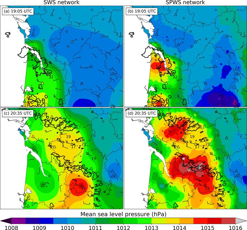
306              M. Mandement and O. Caumont: Contribution of PWSs to the observation of deep-convection features

Figure 6. Number of SWSs (a) and PWSs (b) over metropolitan France on 4 July 2018. Observation counts are binned into approximately
0.2◦ × 0.2◦ bins.

the Fig. 2 of Meier et al. (2017) but with a lower amplitude:       terpolating, for each grid point, weather stations available in
the median remains in the range 0 ◦ C ± 0.5 ◦ C for all hours       the vicinity. The gridding method used is the inverse-distance
of the day. For pressure, some sources of errors exposed by         weighting (IDW) with a power factor of 2. Weather stations
McNicholas and Mass (2018a) in smartphone pressure sen-             too far away from a grid point are not used in the computa-
sors apply to PWS pressure sensors because they are simi-           tion.
lar microelectromechanical systems (MEMS). According to                 Every maximum range is a trade-off between the smallest
their study, errors result from different response times of sen-    possible range that limits the extrapolation of small-scale fea-
sors to pressure changes, sensor bias, inaccurate metadata          tures and a larger range keeping enough stations to limit the
or user-related issues (pressurized environments, below or          influence of a single station over the surrounding grid points.
above ground-level PWS locations). The STMicroelectron-             For our cases, the maximum distance between every pair of
ics MEMS pressure sensor mounted on Netatmo PWS has a               closest SWS sensors is 46 km for relative humidity and 42 km
±1 hPa absolute accuracy (Netatmo, 2019).                           for temperature; for the combined network of SWS and PWS
   Because of the uncertainties affecting PWS measurements          after processing (see Sect. 4) it is 28 km for relative humidity
and the departures observed in comparison to reference mea-         and 21 km for temperature. These values are lower bounds of
surements, an automatic PWS data processing algorithm was           the maximum ranges in order to prevent inland grid points
built. This includes a quality control in pressure, tempera-        from having the value of the closest SWS even if they are not
ture and humidity which is designed to be simple and effi-          at the same location. For the sake of simplicity, an identical
cient whatever the meteorological situation is. The algorithm       radius is chosen for temperature and relative humidity. Thus,
is mainly based on comparisons with a quality-controlled ref-       for temperature and relative humidity, SWSs distant by more
erence network as was done by Meier et al. (2017) and Clark         than 60 km are not taken into account; this radius is set to
et al. (2018). The data processing is performed during the          30 km for PWSs. The choice of 60 km instead of a 50 km ra-
periods of time indicated in Table 1. Cases begin before con-       dius for example is done to take into account more SWSs at
vection initiation and end after convection dissipation of the      each grid point (for a given inland grid point, interpolation
storm systems studied over the area of interest. In order to        uses 9.8 SWSs on average with a 60 km radius compared to
accurately evaluate PWSs and be able to detect abnormal be-         8.6 SWSs on average with a 50 km radius for the 26 May
haviour, calm conditions are necessary for most of the time.        case). For MSLP and surface pressure, SWSs distant by more
Indeed, if storms affect weather stations at each time step,        than 100 km are not taken into account; this radius is also set
conclusions about the quality of the measurements by com-           to 100 km for PWSs. The radius is larger for pressure because
paring it to a reference or close stations may be dubious,          it is the minimum radius for covering the entire metropolitan
given the small scale of some phenomena.                            area of France. This is due to the small number of SWS pres-
                                                                    sure sensors and because stations with an altitude higher than
4.1   Gridding methods                                              750 m are discarded (see Sect. 4.4). A maximum of 10 SWSs
                                                                    and 30 PWSs are used at each grid point in the IDW, an arbi-
For temperature, relative humidity, MSLP and surface pres-          trary limit set to diminish the program execution time.
sure, all gridded analyses derived from observations are built          MSLP and relative humidity are directly gridded (Fig. 7a;
at a 10 min time step and 0.01◦ resolution in latitude and lon-     method [1]). For temperature and surface pressure, because
gitude (≈ 1.1 km N–S and ≈ 0.8 km E–W at 45◦ N) by in-              they vary strongly with altitude, a linear regression of the

Nat. Hazards Earth Syst. Sci., 20, 299–322, 2020                             www.nat-hazards-earth-syst-sci.net/20/299/2020/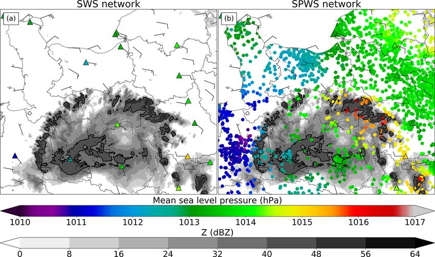
M. Mandement and O. Caumont: Contribution of PWSs to the observation of deep-convection features                                     307

Figure 7. (a) Gridding methods used to build analyses from discrete surface observations. MSLP and relative humidity are gridded using
method [1], while temperature and surface pressure are gridded using method [2]. (b) LOOCV algorithm explained through the case of
four observations made by four weather stations, including two validation stations during one time step. The complete LOOCV is a loop
performed over all time steps (n) and over all validation stations chosen (m). The loop provides an array of errors (j,k )1≤j ≤n,1≤k≤m of
dimension n × m, allowing the computation of a RMSE over n × m observations or a RMSE associated to a validation station only over
n observations. If the estimate is equal to the observation, error is equal to zero.

SWS observations used in the gridding with respect to the
altitude is performed first. After that, the residuals (i.e. the                                   gM
                                                                                             0zPWS − 0R0

difference between the values obtained by linear regres-                     MSLPPWS = P 1 −             ,                            (1)
sion and the observations) are gridded as shown in Fig. 7a                                    T0
(method [2]) and then added to the grid derived from the
linear regression. For temperature, the linear regression is                 where P is the surface pressure measured at the PWS
adapted: to diminish the predominant weight of the low al-                   (in hPa), T0 = 288.15 K is the sea level temperature of
titude SWSs over the highest SWSs, SWSs are binned in                        the International Civil Aviation Organization (ICAO)
vertical layers of 100 m height. The mean temperature and                    standard atmosphere, 0 = 0.0065 K m−1 is the ICAO
the mean altitude of SWSs comprised in each layer are com-                   environmental lapse rate in the troposphere below
puted. A linear regression is then performed over these verti-               11 km, g = 9.80665 m s−2 is the standard acceleration
cal layers. This choice was made to be closest to the observed               of gravity, M = 0.0289644 kg mol−1 is the molar mass
temperature lapse rate rather than using a constant lapse rate.              of dry air and R0 = 8.31447 J mol−1 K−1 is the ideal
   The reference analyses, called SWS analyses, used in the                  gas constant.
following sections are built only with SWS data.                          – Surface pressure P is provided if zPWS is unknown
                                                                            (17 % of cases).
4.2   Computation of PWS MSLP
                                                                       To compare MSLPPWS to SWS measurements, it was neces-
Even when the altitude of the Netatmo PWS (zPWS ) is un-               sary to recalculate the MSLP. The formula used to calculate
known, the PWS still provides a pressure value. In fact, under         the MSLP for SWSs is the one in use at Météo-France and is
the name of pressure, Netatmo provides two different quan-             the same as that used by, for example, Garratt (1984). It takes
tities.                                                                into account the observed surface temperature and humidity
  – It provides a MSLP (MSLPPWS ) computed from the hy-                at the weather station:
    drostatic equation assuming a constant 15 ◦ C tempera-                                                    gM      !
                                                                                                              R0 z

                                                                                          gMz
    ture and a 0 % relative humidity at sea level if zPWS is           MSLP = P exp               = P exp
    known (83 % of cases):                                                               R0 Tv              Tv + 02 z

                                                                                            0.03414z
                                                                               = P exp                    ,                        (2)
                                                                                         Tv + 0.00325z

www.nat-hazards-earth-syst-sci.net/20/299/2020/                                  Nat. Hazards Earth Syst. Sci., 20, 299–322, 2020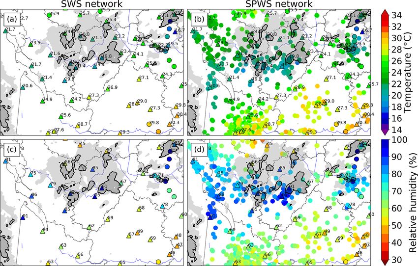
308                  M. Mandement and O. Caumont: Contribution of PWSs to the observation of deep-convection features

with Tv being the mean virtual temperature in the fictitious       the closest to the actual PWS altitude, is used in the compu-
air column extending from sea level to the level of the station,   tation. Residuals time series are taken from the closest grid
which is equal to Tv + 02 z, considering the decrease in the       point residuals. This precise calculation corresponds to SWS
virtual temperature with altitude at a constant lapse rate 0 in    analyses having an accurate ground altitude at PWS loca-
this column.                                                       tions.
   The virtual temperature Tv at the weather station is de-           For each PWS, the median of the errors between the time
rived from T , the 2 m temperature in kelvin (t is T in ◦ C),      series derived from SWS analyses at its location (x a ) and its
                                         U
and the 2 m water vapour pressure e = 100   ew (in hPa) where      raw PWS time series (x r ) is obtained. The corrected PWS
U is the 2 m relative humidity (in %) and ew is the saturation     time series (x c ) is computed by removing the median of the
water vapour pressure (in hPa) obtained through the World          errors from the raw PWS time series:
Meteorological Organization (2014) formula. Tv and ew are
computed as follows:                                               x c = x r − med (x r − x a ) l,                             (4)
            T               T
Tv =                 =         ,                                   with x c , x r , x a and l column vectors gathering a single PWS
            0.378e         0.378U ew
       1−     P   1−         100P                                  time series of dimension n, being equal to the number of time

                        17.62t
                                                                  steps of a case. Here, l = {1, . . . , 1}.
with ew = 6.112 exp                .                        (3)       The choice of the median is explained by the observation
                      t + 243.12
                                                                   of large variations in temperature, humidity or pressure due
T and U are derived from the nearest point of the SWS anal-        to deep convection. Because of the lower density of the SWS
yses. The altitude z is equal to zPWS if the difference in al-     network compared to the PWS network, some of these vari-
titude is less than 15 m between zPWS and the Shuttle Radar        ations that are actual signals affect the calculation of mean
Topography Mission (SRTM; Farr et al., 2007) digital eleva-        error. Using the median allows for ignoring a major part of
tion model (DEM) extracted from Python package “altitude”          these physical deviations while identifying systematic errors
(de Ruijter, 2016). If the difference is larger than 15 m, the     affecting PWSs. This procedure is close to the one followed
DEM altitude is taken. The value is chosen to keep the ben-        by Madaus et al. (2014), which is performed over periods of
efit of accurate altitudes that may be given by internal GPS       several months.
of smartphones to the Netatmo mobile application during the           In the following parts, all PWS time series refer to cor-
PWS set-up process. This results in more accurate altitude         rected PWS time series. The steps leading to these PWS cor-
when the PWS is located in a small building, for example.          rected time series, i.e. the computation of PWS MSLP and
Then, comparing metadata to a DEM eliminates altitude er-          the PWS systematic error correction, are referred to as PWS
rors that may be introduced by users: they may erroneously         preprocessing.
modify PWS altitude because it is a way to modify the value
of PWS pressure.                                                   4.4   PWS data quality control

4.3    PWS systematic error correction                             Two common filters are applied to pressure, temperature and
                                                                   humidity. A PWS is removed if it has the same latitude and
The motivation to compare Netatmo measurements to SWS              longitude as another and less than half of the measurements
analyses is to eliminate systematic errors. Some of them are       are available. For the computation of MSLP, PWSs with al-
due to the PWS itself, such as sensor quality or the impos-        titude higher than 750 m are discarded, as recommended by
sibility of maintenance by design; some are due to the envi-       the World Meteorological Organization (2014). Then a last
ronmental conditions where the PWS is set up, but some are         filter is applied in order to discard PWSs that do not provide
due to PWS owners who can calibrate sensors as they wish.          accurate measurements.
The mobile-phone application allows users to calibrate the             For temperature and relative humidity, the last filter is
temperature sensor and modify the altitude, which has an in-       based on the assumption that the larger the differences be-
fluence on pressure. All sensors can be calibrated by personal     tween PWS time series and SWS analyses during the case
requests to Netatmo.                                               study, and the longer they last, the less confidence is put in
   For relative humidity, PWS time series are compared to          PWS measurements. For each PWS, the root-mean-square
the SWS analyses at the closest grid point. For surface pres-      error (RMSE) of PWSs temperature and relative-humidity
sure and temperature, because they vary rapidly with altitude,     time series (x c ) against time series derived from SWS anal-
which itself varies rapidly with spatial distance in mountain-     yses (x a ) is computed. It is hereafter called RMSEPWS , with
ous regions, the value at the PWS closest grid point may be        n being the number of time steps:
really different of the actual PWS value. That is why PWS
                                                                             v
time series are not compared directly to the SWS analyses                    u1 n
                                                                             u X
at the closest grid point. A more precise calculation is per-      RMSEPWS = t        (x c [j ] − x a [j ])2 .                 (5)
formed: the altitude z previously defined, considered to be                    n j =1

Nat. Hazards Earth Syst. Sci., 20, 299–322, 2020                             www.nat-hazards-earth-syst-sci.net/20/299/2020/
M. Mandement and O. Caumont: Contribution of PWSs to the observation of deep-convection features 309
The filter eliminates PWSs with RMSEPWS higher than an pressure. The suspicious PWS is identified by computing the
adaptive threshold called RMSEthresh : RMSE associated with all validation stations k, k ∈ [1; m],
which is
RMSEPWS > RMSEthresh . (6) v
u1 n
u X
To determine the RMSEthresh , an automatic algorithm based RMSELOOCV,k (p) = t j,k (p)2 . (10)
n j =1
on leave-one-out cross validation (LOOCV; see Fig. 7b) was
built. Consider p surface stations (PWSs and SWSs) pro-
The PWS with the highest RMSELOOCV,k (p) is physically
ducing observations including m validation stations (SWSs
the one which disagrees the most in RMSE with all neigh-
only; p ≥ m). For a given time step j ∈ [1; n], the LOOCV
bour PWSs and SWSs during the case study, which is suspi-
removes one validation observation k ∈ [1; m]. Using p − 1
cious. This station is eliminated. The algorithm stops when
observations (all except the observation k), an estimate at the
RMSELOOCV (p) increases at step s + 1 compared to step s.
removed observation location Ek (p) is computed through
Physically, an increase means that a PWS which was in
the gridding method described in Sect. 4.1. Then, the esti-
strong agreement with at least one neighbour station (PWS
mate is compared to the actual observation Sk , giving an er-
or SWS, called k 0 ) was eliminated at step s. At step s + 1,
ror j,k (p):
k 0 captures some physical process (local low or high) but is
j,k (p) = Ek (p) − Sk . (7) alone in doing it, and so RMSELOOCV,k 0 (p) increases as well
as the RMSE of some PWS around it. As a consequence, the
The process is reproduced over the m validation stations and resulting RMSELOOCV (p) taking into account all PWS con-
the n time steps of the case study, giving an array of m × n tributions increases. This algorithm is well fitted for pressure
errors, from which the LOOCV RMSE is computed: because most of the errors affecting PWSs are uncorrelated,
v and few PWSs provide erroneous values. This will probably
u
u1 1 X n X m not work for other parameters like temperature, whose errors
RMSELOOCV (p) = t j,k (p)2 . (8) may be spatially correlated (errors because of direct radia-
n m j =1 k=1
tion for example). Each step of quality control in MSLP is
detailed in Table 4.
The lower the errors, the closer to the observations the es-
The result of PWS processing is illustrated for temper-
timates are. Thereby, RMSELOOCV (p) can be chosen as a
ature in Fig. 8a, for relative humidity in Fig. 8b and for
metric evaluating the accuracy of the p surface stations from
MSLP in Fig. 9. PWS measurements are compared at dif-
which the estimates are built.
ferent time steps to the SWS analyses before and after pro-
Let x be the unknown RMSEthresh . Then, p(x) is the num-
cessing. In terms of temperature (Fig. 8a), the distribution of
ber of PWSs and SWSs which verify RMSEPWS ≤ x (m is
departures before processing exhibits systematic positive de-
the number of SWSs). The RMSEthresh chosen is the x that
partures with a diurnal cycle. The daily minimum of the me-
minimizes RMSELOOCV (p(x)):
dian departures is reached in the morning between 08:00 and
RMSEthresh = argminx RMSELOOCV (p(x)). (9) 10:00 UTC, after sunrise, and the daily maximum is reached
in the evening or the night between 17:00 and 06:00 UTC in
For large values of x, p(x) tends to the total number of PWSs the 4 July case but also in the other cases not shown. In terms
and SWSs remaining after the two common filters, and so of relative humidity (Fig. 8b), the distribution of departures
RMSELOOCV (p(x)) tends toward large values because al- before processing also exhibits a diurnal cycle, with positive
most all PWSs are kept, including those exhibiting abnormal departures during the day and negative departures during the
behaviours. For small values of x, p(x) approaches m, the night in all cases. In terms of MSLP (Fig. 9), the distribu-
number of SWSs, and RMSELOOCV (p(x)) approaches quite tion of departures before processing seems to exhibit a small
large values because of the small number of SWSs and their diurnal cycle, with departures increasing in the morning and
large spacing. decreasing in the evening. For all parameters, the processing
The resulting RMSEthresh picked up by the algorithm de- shifts the distribution of departures near zero and strongly
pends on the case, varying from 1.10 to 1.45 ◦ C in tempera- decreases the width of the interquartile range of departures.
ture and from 5.5 % to 7.5 % in relative humidity. This shows the efficiency of the algorithm in diminishing de-
For MSLP and surface pressure, instead of a threshold, partures to SWS analyses while keeping features associated
PWSs providing suspicious measurements are eliminated with deep convection, as it was designed for (see Sect. 6).
one by one by an algorithm. This consists of a LOOCV using In real time, we do not have access to the complete time
SWSs and PWSs as validation stations (m = p) that elim- series. A variation in the method that could be applied in
inates one suspicious PWS at each step s. PWSs are used real time is using time series over a rolling period of the
in the validation dataset this time because SWS coverage is 24 last hours ending at the time of the analysis instead of
quite sparse. A one-by-one elimination is possible because the time series over a complete event. Then, every 10 min
only few PWS errors remain after the first three filters in the automatic processing would be launched for each anal-
www.nat-hazards-earth-syst-sci.net/20/299/2020/ Nat. Hazards Earth Syst. Sci., 20, 299–322, 2020310 M. Mandement and O. Caumont: Contribution of PWSs to the observation of deep-convection features
Table 3. Number of PWSs filtered at each step of the quality control in temperature (T ) and relative humidity (U ) over the area of each case
study.
Case study 26 May 2018 4 July 2018 15 July 2018 28 August 2018
T U T U T U T U
Number of PWS time series 11 372 5113 5063 7347
Same latitude–longitude 100 37 32 48
> 50 % missing values 615 616 324 326 296 298 448 448
RMSEPWS > RMSEthresh 6731 6242 2508 2141 3103 2947 4051 4735
RMSEthresh 1.10 ◦ C 6.5 % 1.40 ◦ C 7.5 % 1.45 ◦ C 7.5 % 1.20 ◦ C 5.5 %
PWS remaining 3926 4414 2244 2609 1632 1786 2800 2116
% of total PWS 35 % 39 % 44 % 51 % 32 % 35 % 38 % 29 %
Figure 8. Illustration of the PWS processing in (a) temperature and (b) relative humidity for the 4 July 2018 case. The distribution of
departures between PWS measurements and their corresponding SWS analysis values every 10 min is shown with the 25th quantile (Q25 ),
the median and the 75th quantile (Q75 ). In red are raw PWS time series; in blue are processed PWS time series (time in UTC).
ysis produced. This method implies that the algorithm runs
in less than 10 min, which is not the case for the current al-
gorithm. It takes around 1 h to perform the quality control
over 24 h of measurements on a computer with a central pro-
cessing unit (CPU) with four cores and 16 GB of random-
access memory. To increase the processing speed, one or sev-
eral available computing nodes with 24 cores each could be
used because the algorithm is partially parallel. Parts of the
algorithm that are still sequential could be parallelized. In
addition, the LOOCVs in the quality control could be modi-
fied because there are the most time-consuming parts of the
algorithm. For temperature and humidity, LOOCVs provide
thresholds, and for pressure the LOOCV eliminates a small
number of PWSs one by one. Thus, the algorithm at a given
Figure 9. Illustration of the PWS processing in MSLP for the time can use the temperature and humidity thresholds as well
26 May 2018 case. The distribution of departures between PWS as the list of PWSs eliminated that were computed by the al-
measurements and their corresponding SWS analysis values every gorithm launched 1 h before.
10 min is shown with Q25 , the median and Q75 . In red are raw PWS
time series, in green are preprocessed PWS time series and in blue
are processed PWS time series (time in UTC). 5 Validation
After PWS time series were processed, the remaining PWSs
were combined to SWSs. This network is called hereafter
Nat. Hazards Earth Syst. Sci., 20, 299–322, 2020 www.nat-hazards-earth-syst-sci.net/20/299/2020/M. Mandement and O. Caumont: Contribution of PWSs to the observation of deep-convection features 311
Table 4. Number of PWSs filtered in MSLP at each step of the quality control for each case study.
Case study 26 May 2018 4 July 2018 15 July 2018 28 August 2018
Number of PWS time series 13 098 5820 5783 8432
Identical latitude–longitude 107 41 36 56
> 50 % missing values 523 316 277 431
Altitude > 750 m 7 175 165 105
LOOCV removal algorithm 155 81 80 65
PWS remaining (% of PWS time series) 12 306 (94 %) 5207 (89 %) 5225 (90 %) 7775 (92 %)
the standard and personal weather stations (SPWS) network experiments compared to SWS experiments. Bias reaches
(Fig. 10), and the gridded fields produced with this network 0.74 to 1.45 ◦ C, and the increase in RMSE ranges from 41 %
are called SPWS analyses. The additional value of SPWS to 72 % compared to SWS experiments. These results show
analyses compared to SWS analyses is evaluated quantita- the key role of processing: without this step, adding PWSs
tively in MSLP, temperature and relative humidity. Also, for strongly decreases the quality of analyses.
temperature and relative humidity, in order to evaluate the For SPWS experiments, a decrease ranging from 0.00 to
role of processing in the results obtained, raw PWS time se- 0.04 ◦ C in absolute value of the median error is observed
ries and SWS time series were combined. The network asso- compared to SWS experiments, depending on the case. The
ciated to this dataset is called the SPWS_raw network. It is absolute value of the mean error shows no particular trend
not done for pressure because the raw dataset blends MSLP and remains less than 0.07 ◦ C for all cases in SPWS exper-
and surface pressure as explained in Sect. 4.2. iments. This indicates that PWSs do not introduce substan-
LOOCVs are performed on SWS, SPWS and SPWS_raw tial bias or shifts in the temperature distribution. A decrease
observations (p observations) and validated on SWS obser- ranging from 0.06 to 0.22 ◦ C in the interquartile range of er-
vations (m observations) included in these datasets. The me- rors is observed for all cases in SPWS experiments compared
dian of j,k (p) over all validation stations k ∈ [1; m] and to SWS experiments. Also, a substantial decrease in RMSE
all time steps j ∈ [1; n] is computed. The RMSELOOCV (p) ranging from 12 % to 23 % is observed. These results quan-
is also computed and corresponds to the line labelled RMS titatively show that adding PWS measurements in tempera-
(root mean square) in the tables. The mean and quartiles ture analyses improves their accuracies. For temperature, the
of j,k (p), not shown in the tables, have also been scruti- number of available observations is multiplied by 11 on av-
nized. All experiments are compared to the SWS experiment. erage over the four cases with the SPWS network compared
to the SWS network.
5.1 MSLP
5.3 Relative humidity
In MSLP (Table 5), a decrease ranging from 0.01 to 0.05 hPa
in absolute value of the median error is observed in SPWS In relative humidity (Table 7), shifts of the median error rang-
experiments compared to SWS experiments, depending on ing from −3.3 % to 2.7 % are observed in SPWS_raw exper-
the case. The absolute value of the mean error decreases in iments compared to SWS experiments. Biases reach −2.3 %
three cases and remains stable in one case: it is less than to 1.9 %, and RMSEs increase from 6 % to 31 % compared
0.02 hPa for all cases in SPWS experiments. A decrease rang- to SWS experiments. These results show the key role of pro-
ing from 0.32 to 0.48 hPa in the interquartile range of er- cessing: without this step, adding PWSs strongly decreases
rors is observed for all cases in SPWS experiments com- the quality of analyses.
pared to SWS experiments. Also, a very substantial decrease For SPWS experiments, the absolute value of the median
in RMSE ranging from 73 % to 77 % is observed. These re- error is less than or equal to 0.2 % and the absolute value
sults quantitatively show that adding PWS measurements in of the mean error remains less than 0.6 %. This indicates
observed MSLP analyses strongly improves their accuracy. that PWSs do not introduce any substantial bias or shifts in
For MSLP, the number of available observations is multi- the relative-humidity distribution. A decrease ranging from
plied by 134 on average over the four cases with the SPWS 0.0 % to 1.9 % in the interquartile range of errors is observed
network compared to the SWS network. for all cases in SPWS experiments compared to SWS exper-
iments. Also, a substantial decrease in RMSE ranging from
5.2 Temperature 17 % to 21 % is observed. These results quantitatively show
that adding PWS measurements in relative-humidity analy-
In temperature (Table 6), a positive shift of the median er- ses improves their accuracies. For relative humidity, the num-
ror ranging from 0.73 to 1.39 ◦ C is observed in SPWS_raw ber of available observations is multiplied by 14 on average
www.nat-hazards-earth-syst-sci.net/20/299/2020/ Nat. Hazards Earth Syst. Sci., 20, 299–322, 2020312 M. Mandement and O. Caumont: Contribution of PWSs to the observation of deep-convection features
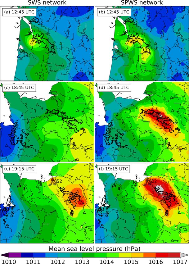
Figure 10. MSLP observations of (a) SWS network and (b) SPWS network at 18:15 UTC on 26 May. SWSs are indicated by coloured
triangles with black contours and PWSs by coloured circles. The instantaneous wind gust is shown with barbs. Base reflectivity (Z) in grey
colours indicates thunderstorm activity and location. Reflectivities over 40 dBZ are illustrated with bold black contours.
Table 5. Statistics of the LOOCV performed on SWS and SPWS observations of MSLP and validated on SWS observations for each case
study. The evolution (in %) is relative to the RMSE of SWS observations.
Case study 26 May 2018 4 July 2018 15 July 2018 28 August 2018
Network SWS SPWS SWS SPWS SWS SPWS SWS SPWS
Median 0.012 −0.001 0.015 −0.002 0.030 −0.002 0.048 0.002
MSLP error (hPa)
RMS 0.404 0.099 0.702 0.187 0.449 0.104 0.611 0.151
% of evolution −7 % −73 % −77 % −75 %
over the four cases with the SPWS network compared to the 6.1 Contribution of PWSs to MSLP analyses
SWS network.
6.1.1 26 May 2018
5.4 Sensitivity to the gridding method
At 12:45 UTC on 26 May 2018, a squall line was located
To study the sensitivity to the gridding method, we slightly over the south-west of France. The MSLP field of SWS
modified the gridding method for the 26 May case. The analysis (Fig. 11a) exhibits a single pressure high, reaching
power factor of the IDW was set to 1 instead of 2. We 1014.9 hPa, in the western part of the MCS, south of the high-
observe little sensitivity to the change of the power factor. est reflectivities. It does not show significant pressure pertur-
With a power factor of 1 (respectively 2), for SPWS the bations or strong pressure gradients in the eastern part of the
MSLP RMSE equals 0.118 hPa (0.099 hPa), the temperature MCS. In SPWS analysis (Fig. 11b), a crescent-shaped pres-
RMSE equals 0.877 ◦ C (0.889 ◦ C) and the relative-humidity sure high associated with the system is identified in MSLP,
RMSE equals 5.480 % (5.375 %). Decreases in RMSE reach reaching 1015.0 to 1015.5 hPa, especially near and under the
70 % (75 %) in MSLP, 16 % (16 %) in temperature and 17 % highest reflectivities in the convective part of the storm. A
(21 %) in relative humidity with SPWS compared to SWS. MSLP low is located at the rear of the stratiform part. Along
the strong pressure gradients revealed by the SPWS network,
high wind gusts of 19 m s−1 at 12:10 UTC and 25 m s−1 at
6 Results for selected convective cases 12:38 UTC were observed in the eastern part of the MCS.
The MSLP field agreeing the most with MSLP anomalies de-
In the following section, comparisons are made between scribed by the theory of squall lines (Johnson and Hamilton,
SWS and SPWS networks by showing observed values at 1988; Haertel and Johnson, 2000) is found in SPWS analysis.
station locations or by comparing SWS and SPWS analyses. SPWS analysis is also more coherent with surface wind ob-
Nat. Hazards Earth Syst. Sci., 20, 299–322, 2020 www.nat-hazards-earth-syst-sci.net/20/299/2020/You can also read