Production and excitation of molecules by dissipation of two-dimensional turbulence
←
→
Page content transcription
If your browser does not render page correctly, please read the page content below
MNRAS 495, 816–834 (2020)                                                                                                          doi:10.1093/mnras/staa849

Production and excitation of molecules by dissipation of two-dimensional
turbulence

P. Lesaffre ,1‹ P. Todorov,1 F. Levrier,1 V. Valdivia ,2 N. Dzyurkevich,3 B. Godard,1
L. N. Tram,4,5 A. Gusdorf,1 A. Lehmann 1 and E. Falgarone1
1 Laboratoire   de Physique de l’ENS, ENS, Université PSL, CNRS, Sorbonne Université, Université Paris-Diderot, Paris, France
2 Laboratoire   AIM, Paris-Saclay, CEA/IRFU/SAp - CNRS - Université Paris Diderot, 91191 Gif-sur-Yvette Cedex, Franc
3 Institute for Theoretical Astrophysics (ITA), University of Heidelberg, Albert-Ueberle Str., 69120 Heidelberg, Germany
4 SOFIA-USRA, NASA Ames Research Center, Ms 232-11, Moffett Field, CA 94035, USA

                                                                                                                                                               Downloaded from https://academic.oup.com/mnras/article/495/1/816/5841083 by guest on 20 September 2020
5 University of Science and Technology of Hanoi, VAST, 18 Hoang Quoc Viet, Hanoi, Vietnam

Accepted 2020 March 17. Received 2020 March 16; in original form 2019 July 8

                                         ABSTRACT
                                         The interstellar medium (ISM) is typically a hostile environment: cold, dilute and irradiated.
                                         Nevertheless, it appears very fertile for molecules. The localized heating resulting from
                                         turbulence dissipation is a possible channel to produce and excite molecules. However,
                                         large-scale simulations cannot resolve the dissipative scales of the ISM. Here, we present two-
                                         dimensional small-scale simulations of decaying hydrodynamic turbulence using the CHEMSES
                                         code, with fully resolved viscous dissipation, time-dependent heating, cooling, chemistry and
                                         excitation of a few rotational levels of H2 . We show that molecules are produced and excited
                                         in the wake of strong dissipation ridges. We carefully identify shocks and we assess their
                                         statistics and contribution to the molecular yields and excitation. We find that the formation
                                         of molecules is strongly linked to increased density as a result of shock compression and
                                         to the opening of endothermic chemical routes because of higher temperatures. We identify
                                         a new channel for molecule production via H2 excitation, illustrated by CH+ yields in our
                                         simulations. Despite low temperatures and the absence of magnetic fields (favouring CH+
                                         production through ion-neutral velocity drifts), the excitation of the first few rotational levels
                                         of H2 shrinks the energy gap to form CH+ . The present study demonstrates how dissipative
                                         chemistry can be modelled by statistical collections of one-dimensional steady-state shocks.
                                         Thus, the excitation of higher J levels of H2 is likely to be a direct signature of turbulence
                                         dissipation, and an indirect probe for molecule formation. We hope these results will help to
                                         bring new tools and ideas for the interpretation of current observations of H2 rotational lines
                                         carried out using the Stratospheric Observatory for Infrared Astronomy (SOFIA), and pave
                                         the way for a better understanding of the high-resolution mapping of H2 emission by future
                                         instruments, such as the James Webb Space Telescope and the Space Infrared Telescope for
                                         Cosmology and Astrophysics.
                                         Key words: astrochemistry – diffusion – hydrodynamics – shock waves – ISM: kinematics
                                         and dynamics – ISM: molecules.

                                                                                  large temperature thresholds, such as for CH+ and SH+ , to be
1 I N T RO D U C T I O N
                                                                                  overcome (see Nehmê et al. 2008; Godard et al. 2012). Besides, the
Although the diffuse interstellar medium (ISM) is cold and dilute, it             excitation of high levels of the molecules such as H2 is observed
appears to be quite fertile in the production of molecules, even when             despite the low average temperature of this medium (see Gry et al.
the formation of molecules needs adverse dissociating radiation or                2002; Falgarone et al. 2005; Ingalls et al. 2011). Non-thermal
                                                                                  phenomena might help to overcome the formation thresholds
                                                                                  for these molecules. For instance, the interstellar radiation field
                                                                                 ionizes the medium and opens molecular formation routes through
    E-mail: pierre.lesaffre@ens.fr

                                                                                                                                     C The Author(s) 2020.

Published by Oxford University Press on behalf of The Royal Astronomical Society. This is an Open Access article distributed under the terms of the Creative
Commons Attribution License (http://creativecommons.org/licenses/by/4.0/), which permits unrestricted reuse, distribution, and reproduction in any medium,
                                                                                                               provided the original work is properly cited.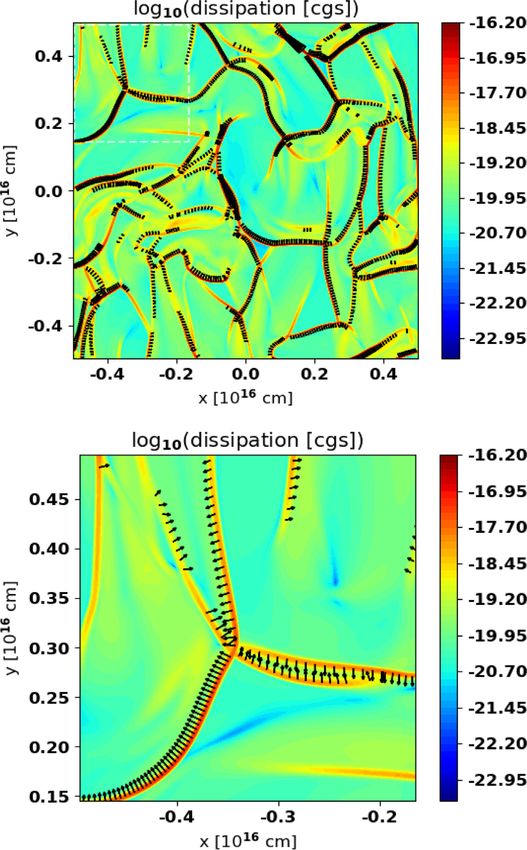
Molecular excitation in decaying turbulence                       817
hydrogenation of the O+ cation, provided the ultraviolet (UV)               refinement (Teyssier 2002; Fromang, Hennebelle & Teyssier 2006).
irradiation field is not too strong and that the H2 molecule remains        DUMSES uses the MHD solver of RAMSES on a regular grid (i.e.
unhindered. This was investigated in detail by Levrier et al. (2012),       without the adaptive mesh part). We use Van-Leer slopes to estimate
who found that, for the standard irradiation field and for the densities    the right and left states of the Riemann solver, for which we
around 100 cm−3 in the diffuse ISM, their models underpredict the           approximate the fluxes by the Lax–Friedrich prescription (see Toro
observed line fluxes and column densities of molecules. Molecules           1999). The regular grid makes it much easier to implement new
are too fragile for the diffuse medium irradiation and additional           physics in DUMSES, especially dissipation and diffusion terms,
physical processes are needed to increase their abundances, such            which require easy access to neighbouring zones. Therefore, it
as ion-neutral drift (as in C-type shocks; see Flower, Pineau des           makes it simpler to quickly explore and validate a variety of new
Forêts & Hartquist 1985), turbulent diffusion (Lesaffre, Gerin &           methods.
Hennebelle 2007) or turbulent dissipation (Godard, Falgarone &                 We added in DUMSES the treatment of dissipative terms (viscous
Pineau Des Forêts 2009).                                                   momentum diffusion, thermal diffusion and chemical diffusion) as
   Shock compression leads to larger densities and hence more               cell-centred differences, which makes them second-order accurate

                                                                                                                                                      Downloaded from https://academic.oup.com/mnras/article/495/1/816/5841083 by guest on 20 September 2020
efficient formation rates. The dissipation of turbulence, even when         in space. We bracket the Godunov step with two half dissipation
it is incompressible, can bring the medium to high temperature              steps, one before and one after, in order to retain the second-order
in sharply localized dissipative structures (Falgarone, Pineau des          accuracy in time of the original scheme (we summarize the resulting
Forets & Roueff 1995). Pioneering work by Joulain et al. (1998) and         scheme in Section 2.3). A constraint using the minimum of all
Godard et al. (2009) showed that incompressible dissipation could           diffusion times across each cell is added to the usual time-step
be effective at producing molecules and reproducing observational           control. Note that, in the present application, we use the same
trends.                                                                     coefficient for momentum, chemical and thermal diffusion, so these
   In the present study, we aim to explore dissipative chemistry            time-scales are all the same. This approximation reflects the fact
further. We run a multidimensional numerical experiment that                that all three diffusion mechanisms proceed through molecular
renders some of the complexity of the ISM chemistry while fully             collisions, and we assume that the carriers have the same mean
resolving the dissipation scale. We attempt to characterize some            mass for all three mechanisms. Likewise, we implement resistivity
of the processes that lead from dissipation to new molecules. In            and validate the dissipative terms using Alfvén waves tests, as
particular, we decompose a snapshot of decaying turbulence into             described in Lesaffre & Balbus (2007). In particular, we verify
individual one-dimensional (1D) steady planar shocks. We then               the quadratic convergence with respect to both time and space
proceed to demonstrate that this collection of shocks allows us             resolution. Chemical diffusion is also tested in simple 1D reaction–
to account for most of the dissipation, excitation and molecular            diffusion steady-state shock fronts. The current version of the code
content in the simulation. This simplified experiment creates a link        can accommodate magnetic fields, but the present application does
between complex dynamics and a statistical collection of 1D steady-         not consider them.
state shocks. The 1D steady-state shock models can in the future               The implementation of viscosity used in this paper assumes con-
be improved at will by using more refined chemistry and thermal             stant kinematic viscosity ν rather than constant dynamic viscosity
processes, more appropriate to match observational requests.                μ = νρ, where ρ is the mass density of the fluid. The latter
   Our study is the first to include time-dependent excitation of           is appropriate for isothermal gases and assumes that the mean
H2 in multidimensional hydrodynamics. This allows us to uncover             free path scales inversely proportional to ρ. While the former
another potential means to favour molecule formation, because of            might not be reasonable for the ISM, we believe that as long
lowered temperature thresholds due to the energy stored in excited          as the collisional time-scales are smaller than the thermal and
H2 . As a first step, we focus here on a two-dimensional (2D)               chemical time-scales, thermochemistry is not affected. However,
configuration without magnetic fields. In particular, we do not yet         our assumption of constant ν assumes that the mean free path is
include ambipolar drifts, which are known to favour neutral-ion             a constant. This ensures more homogeneous dissipation length-
chemical routes.                                                            scales and helps us foresee the necessary resolution. Besides, the
   In Section 2, we introduce the CHEMSES code and we give details          steady-state shock fronts offer an analytical solution in that case
of our numerical set-up. In Section 3, we show the results of the           (see Appendix A2), which simplifies the shock extraction we use
numerical experiment: the effects of turbulent dissipation on the           in the analysis of our results. The successful comparison of the
average thermodynamical and chemical state of the gas and its H2            steady-state shocks with the analytics provides an extra validation
excitation diagram. In particular, we show how excitation can affect        of the viscous term’s implementation (see Appendix A3).
some of the chemistry. In Section 4, we explore in detail the role of
shocks in our simulation, and how we can recover some of the results
                                                                            2.2 The Paris–Durham steady-state shock code
of the previous section with a well-chosen collection of 1D planar
shocks. In Section 5, we discuss our conclusions and prospects for          The Paris–Durham shock code solves the 1D MHD equations in a
the future.                                                                 steady-state frame. It integrates the dynamical, thermal, excitation
                                                                            state and chemical history of fluid particles as they enter a planar
                                                                            steady-state shock (cf. Flower et al. 1985, 2003; Lesaffre et al. 2013;
2 NUMERICAL METHOD                                                          Flower & Pineau des Forêts 2015). For more than 30 yr, the cooling
                                                                            functions, the chemistry and the grain physics have been refined
2.1 The DUMSES hydrodynamics solver                                         as the shock models were compared with various observations.
DUMSES,1   mainly written by S. Fromang, originates from RAM-               The included heating and cooling processes are atomic cooling
SES,   a magnetohydrodynamics (MHD) code with adaptive mesh                 (such as Lyman α, C+ , C, O), molecular cooling (H2 , CO, OH,
                                                                            H2 O), cosmic ray ionization heating and photoelectric heating.
                                                                            Collisional exchanges between gas and grains are also included
1 Or ‘RAMSES   for the dummies’.                                            but the grain temperature is kept constant and is a parameter

                                                                                                                  MNRAS 495, 816–834 (2020)
818       P. Lesaffre et al.
of the problem (set to 15 K). The Paris–Durham shock code                  (ii) half a thermo-chemical step (isochoric evolution of pressure,
makes use of a highly modular set of chemical reactions including        chemical species and H2 populations);
two-body gas phase reactions, photoionization, photodissociation,          (iii) one hydrodynamical step (classic Godunov step);
H2 formation on grain surfaces, cosmic ray induced ionization,             (iv) half a thermo-chemical step;
desorption, secondary photon ionization and dissociation, grain            (v) half a dissipation and diffusion step.
sputtering and erosion. The code uses DVODE (Brown, Byrne &
Hindmarsh 1989) as its time integration engine. The population           Thermochemistry can potentially affect the dynamics. For example,
of excited levels of H2 is followed in a time-dependent fashion,         ionization or dissociation increases the total number of particles,
coupled to the fluid dynamics, which allows direct predictions for       and hence the pressure. The time-step control should reflect this
the H2 line intensities.                                                 constraint. We record the relative pressure variation during each
                                                                         thermochemical step. If the relative pressure change due to thermo-
                                                                         chemistry is larger than 5 per cent, we reduce the following time-step
                                                                         to satisfy the constraint. Otherwise, we use the minimum between

                                                                                                                                                  Downloaded from https://academic.oup.com/mnras/article/495/1/816/5841083 by guest on 20 September 2020
2.3 Coupling DUMSES and Paris–Durham                                     the diffusive and Courant–Friedrichs–Lewy (CFL) conditions. We
DUMSES    can incorporate a number of passive scalars, which are         multiply the resulting time by 0.7 and set it to the next time-step
evolved alongside the dynamical variables. We make room for the          for more safety. In our applications, the most stringent constraint is
chemical tracers (a total number of 40 species) and the excited          usually given by the CFL condition, so we effectively function at a
levels of H2 (seven levels), which will be taken care of by the Paris–   Courant number (i.e. the ratio between the time-step and the CFL
Durham code: a total of 47 scalars on top of the four dynamical          maximum stable time step) of 0.7.
variables (density ρ, total energy E and the two components of              As noted by several authors (Plewa & Müller 1999; Glover
the velocity). We interfaced Paris–Durham to compute only the            et al. 2010), non-linear evolution and advection of the set of
isochoric time evolution of a single gas temperature, chemical           chemical species does not retain constant elemental composition.
abundances and excited levels population of H2 . The time evolution      In particular, Glover et al. (2010) designed a scheme called
of internal energy and scalars (‘thermochemistry’) is delegated to       the modified consistent multifluid advection (MCMA) to recover
Paris–Durham at each time-step for each zone of the simulation.          multiple elemental conservation constraints in a set of species. We
The irradiation conditions are assumed to be uniform, which sets a       extend this method to the H2 level populations such that the sum
maximum extension for the computational box; the visual extinction       of the populations of excited H2 levels has to match the H2 number
across the box should not exceed about 0.01 mag.                         density. We apply it to the vector of chemical scalars after each
   We use the seven lowest levels of H2 up to a transition energy        thermochemical step, and on the Godunov fluxes of the chemical
of 3474 K, close to the energy threshold for CH+ formation (see          scalars, before they are advected.
Section 3.4.5). The largest rotational number Jmax = 6 is indeed            The DVODE solver for the whole set of thermochemical variables
chosen to target the energy gap for the CH+ formation: this was          is CPU-intensive. For each pixel, we evaluate the initial thermo-
also adopted in early C-type shock studies by Flower & Pineau des        chemical time-scale at the beginning of each thermochemical step
Forets (1998). We have also checked, for a 1D steady-state shock at      by computing the shortest evolution time-scale between all scalars
2 km s−1 , that Jmax = 6 is sufficient to give converged temperature     and the temperature. We decide to resort to DVODE only if this
and H2 excitation profiles compared to Jmax = 150. However, we           evolution time-scale is shorter than 10 times the hydrodynamical
note that the chemical profile of CH+ in this shock is very slow         step (i.e. when the thermochemical evolution is stiff). Otherwise,
to converge with respect to Jmax , with its maximum abundance            the evolution for this pixel is slow enough that we can use a much
enhanced by a factor of 2 between Jmax = 6 and Jmax = 150 (see           faster Runge–Kutta method of order 2 without loss of accuracy.
Section 3.4.5).                                                          This saves a considerable amount of CPU time, as a signifi-
   We adopt the same minimal network of 32 gas species as in             cant fraction of the simulation volume has slow thermochemical
Lesaffre et al. (2004a), necessary to model the abundance of the         evolution.
cooling agents of the ISM: H, C+ , C, O, H2 , CO, OH and H2 O. It           To further reduce CPU consumption, we switch all atomic
is complemented by eight variables necessary to model grain cores        coolants off except for the C+ ion, which often dominates cooling
and their mantles, as in Flower et al. (2003), which brings the total    in the conditions of diffuse ISM (see fig. 3b of Wolfire et al.
number of chemical variables to 40. The resulting network consists       1995, for instance). In particular, we switch off atomic O cooling,
of 172 reactions. As in Lesaffre et al. (2013), the computation of       although we know it can be important in low velocity shocks (see
the rate of the ion-neutral reaction C+ + H2 → CH+ + H takes             Lesaffre et al. 2013). This means that the temperature in the cooling
advantage of the state by state description of the H2 populations        layers of the shocks is slightly overestimated, which results in
and we follow the prescription of Gerlich, Disch & Scherbarth            slightly longer relaxation scales behind the adiabatic fronts (by
(1987), as advocated in Agúndez et al. (2010).                          30 per cent on a shock of about 2 km s−1 ). For a fair comparison,
   In order to retain second-order accuracy in time for the whole        we retain this approximation in both the multidimensional runs
time-step, we split thermochemistry and hydrodynamics by starting        and in the steady-state runs of the Paris–Durham code. Indeed,
with half a time-step for thermochemistry, followed by one full          the main purpose of the present study is to demonstrate the role
hydrodynamical step, and then half a thermochemical step. To retain      of shocks in multidimensional turbulent dissipation. Future work
the necessary symmetry required by second-order time-integration,        on 1D steady-state shocks can strive to refine the observationally
we placed the two half-steps for the dissipation processes wrapped       relevant microphysics.
around this hybrid hydrodynamical and thermochemical time-step.             We refer to the resulting code as CHEMSES, which thus joins the
Thus, the final ordering of the time-step is as follows:                 group of multidimensional codes that couple MHD and chemistry,
                                                                         such as ASTROBEAR (Poludnenko, Frank & Blackman 2002), PLUTO
   (i) half a dissipation step (momentum, chemical and thermal           (Mignone et al. 2007), KROME (Grassi et al. 2014) and NIRVANA
diffusion);                                                              (Ziegler 2005, 2018). Our code is one of the few that control

MNRAS 495, 816–834 (2020)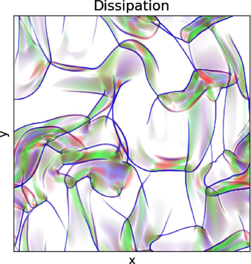
Molecular excitation in decaying turbulence                         819
the dissipation and diffusion physics exactly. To our knowledge,                Table 1. Physical parameters of the simulation.
it is the only code that considers the time dependence of the H2
level populations. The way we interfaced DUMSES with Paris–                     Parameter                                           Value
Durham makes it easy to validate CHEMSES against steady-state                   Average density                                nH = 100 cm−3
shock code computation (see Appendix A1). To our knowledge,                     Domain size                                      L = 1016 cm
this is the first existing test of the coupling between hydrody-                Resolution                                       10242 pixels
namics and thermochemistry. Previously existing codes usually                   Pixel size                                      9.7 × 1012 cm
performed only pure advection tests, which do not test the whole                Temperature at t = 0                              T0 = 66 K
extent of the interplay between chemistry, thermal evolution and                Adiabatic sound speed at t = 0                cs0 = 0.67 km s−1
dynamics.                                                                       rms velocity at t = 0                         urms = 2.1 km s−1
                                                                                rms initial Mach number                         urms /cs0 = 3.1
                                                                                Initial turnover time-scale                         1500 yr
2.4 Simulation parameters                                                       Total duration of the simulation                   10 000 yr
                                                                                Reynolds number at t = 0                     Re = Lurms /ν = 2100

                                                                                                                                                      Downloaded from https://academic.oup.com/mnras/article/495/1/816/5841083 by guest on 20 September 2020
2.4.1 Length-scales and resolution                                              UV irradiation field (Draine’s units)               G0 = 1
                                                                                Visual extinction                               Av = 0.1 mag
Our objective is to test whether turbulence dissipation can po-
tentially produce molecules and excite them even in a diffuse,
moderately shielded medium. Levrier et al. (2012) have shown that            and the molecular yields by 1D planar shocks (see Section 4),
photon-dominated region (PDR) model predictions for CO column                provided the same value of ζ is used in both cases.
densities fall short of a factor of 10 for lines of sight where N(H2 ) is
around a few 1020 cm−2 (see their fig. 11, for example), typical of the
                                                                             2.4.3 Initial composition
diffuse ISM. These diffuse ISM conditions correspond to a density
around nH = 100 cm−3 , which we adopt as our average density. For            Elemental composition is similar to that used in Lesaffre et al.
molecular gas and 10 per cent He in number, this translates to a             (2013). The H2 levels are initialized with separate Boltzmann
total number density of particules of ntot = 60 cm−3 .                       equilibria for ortho levels, on the one hand, and para levels, on
   For this density, the elastic collision mean free path is of              the other hand. We pre-initiate the ortho-to-para ratio to the value
the order of λMFP ∼ 1015 cm−2 /ntot ∼ 1.7 × 1013 cm (see                     of 3 and we integrate chemistry, H2 excitation and thermal evolution
Monchick & Schaefer 1980). Given the √          typical adiabatic sound      during 107 yr from atomic conditions. This provides a first guess
speed in this diffuse medium (about cs = γ p/ρ ∼ 0.8 km s−1 at               near chemical and thermal equilibrium as initial conditions for our
a temperature around 100 K), this sets the viscous coefficient to            hydrodynamic run. During the time interval of pre-initial conditions,
a value around ν ∼ cs λMFP ∼ 1018 cm2 s−1 . The other diffusive              the ortho-to-para ratio drops from 3 to a minimum of 0.2 after
coefficients (chemical and thermal) are also set to this value (see          6 × 10⁵ yr before slowly rising towards its equilibrium value of 1.5.
Section 2.1).                                                                At the end of the pre-initialization time of 107 yr, the ortho-to-para
   We focus our study on one periodic simulation box of decaying             ratio has reached the value of 0.67, which is hence adopted at the
2D turbulence. We can thus afford a domain size of N = 1024 pixels           beginning of the 2D simulation.
aside for a total CPU time of about 100 000 h during six initial
turnover time-scales (tturnover = L/urms; see Table 1). Convergence
studies for both the viscous term (see Appendix A3) and the                  2.4.4 Initial velocity field
chemical term point towards a resolution such that L ∼ Nν/u,                We seed turbulence with an initial random solenoidal velocity field.
where u is the typical shock speed jump (which we take as u                Fourier modes have random phase and uniform amplitude between
∼1 km s−1 ). Therefore, we limit the physical size of our domain to          wavenumber k0 and 5k0 in units of the fundamental mode of the box
L = 1016 cm. This is more than three orders of magnitude smaller             (k0 = 2π /L). As a result, the initial power spectrum (proportional
than typical sizes of diffuse clouds, but it is the price to pay in order    to k times the amplitude of modes in a 2D geometry) peaks at 5k0 .
to resolve the dissipation scale of the diffuse ISM (100 au) in our             We then scale the initial absolute amplitude for the velocity field
simulation.                                                                  such that its root mean square (rms) is urms = 2.1 km s−1 . Our
                                                                             experiment describes a very small region as if it had just flown
                                                                             through a much larger scale dissipative structure. It gets a sudden
2.4.2 Irradiation conditions
                                                                             kick and we observe it during a few thousand yr as it relaxes back
The irradiation conditions are those of the diffuse ISM: standard            to a quiescent state close to the initial conditions. We stop the
stellar irradiation field (ISRF; Draine 1978) mildly shielded by             simulation at a time t = 104 yr, which corresponds to slightly more
an external buffer of visual extinction thickness Av0 = 0.1 mag,             than six initial turnover times L/urms (see Table 1 for a summary of
free of CO but with a column density of 1020 cm−2 of H2 molecules            the main physical parameters). Note that the rms velocity averaged
which provides strong self-shielding to the dissociation of molecular        over the whole duration of the simulation is 0.5 km s−1 , consistent
hydrogen (see Lesaffre et al. 2013). This medium is thus expected            with the higher end of rms velocity observations at a length-scale of
to contain H2 , but be deprived of other molecules. For historical           L = 1016 cm (see fig. 6 in Falgarone, Hily-Blant & Pety 2009). We
reasons, the cosmic ray ionization rate was set to a value ζ =               also tested a two times lower initial rms velocity (see Section 4.5).
3 × 10⁻¹⁷ s−1 ; this is now about 10 times lower than the currently
accepted standard rate at these H2 column densities (see Indriolo,
                                                                             3 R E S U LT S
Fields & McCall 2015; Neufeld & Wolfire 2017, fig. 6). This
may change the H+    3 chemistry essentially in such a way that its
                                                                             3.1 Average behaviour
abundance will be proportional to ζ (see Section 3.4.2). However, it
will presumably not affect the comparison between our simulations            Fig. 1 displays the evolution of the volume-averaged, maximum

                                                                                                                        MNRAS 495, 816–834 (2020)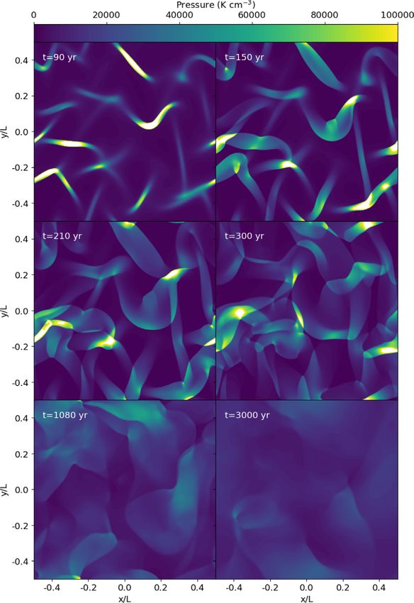
820        P. Lesaffre et al.

                                                                                                                                                             Downloaded from https://academic.oup.com/mnras/article/495/1/816/5841083 by guest on 20 September 2020
                                                                             Figure 3. Time evolution of averaged specific energies: kinetic (solid line),
Figure 1. Time evolution of the volume-averaged temperature (solid line).
                                                                             thermal (dashed line), internal (excitation energy of H2 , dotted line) and
The minimum and maximum values of the temperature are shown as dotted
                                                                             the sum of all three (dash-dotted line). Values are expressed in km2 s−2 .
and dashed lines, respectively. Thin vertical lines mark three epochs of
                                                                             Reference times are indicated as in Fig. 1.
reference: I at t = 300 yr, II at t = 1100 yr and III at t = 3000 yr.
                                                                             3.1.1 Energetics
                                                                             Fig. 3 displays the evolution of three components of the total
                                                                             specific energy:

                                                                                (i) the kinetic energy Ekin = (1/2)ρu2 / ρ, where ρ is the
                                                                             mass density, u is the magnitude of the velocity and angular brackets
                                                                             denote an average over the computational domain;
                                                                                (ii) the thermal energy Eth = (3/2) p / ρ where p is the
                                                                             thermal pressure;
                                                                                      the internal energy, carried by the excitation of H2 molecules:
                                                                                (iii)
                                                                             Eint = JJ =6 =1 nJ (H2 ) EJ / ρ, where nJ (H2 ) is the number density
                                                                             of H2 molecules in the Jth excited level (with vibrational number
                                                                             v = 0 and rotational number J) and EJ is the energy of this level
                                                                             above ground state (we adopt the convention E0 = 0).
                                                                             Thermal versus kinetic energy equipartition is reached very early at
                                                                             t = 270 yr. Kinetic energy then decays very quickly, but energy is
                                                                             stored in thermal and internal components for a much longer time
                                                                             before it is radiated away.
Figure 2. Time evolution of the averaged density (solid line). The minimum      The evolution of kinetic energy is determined by dissipative and
and maximum values of the density are shown as dotted and dashed lines,      compressive heating (Fig. 4) and expressed by
respectively. Reference times are indicated as in Fig. 1.
                                                                                  ∂Ekin
                                                                              −             = − p∇ · u +  viscous  +  numerics  .       (1)
                                                                                    ∂t
and minimum temperature during the simulation. The maximum                   Here, we explicitly separate the total dissipation into a physical
temperature has a very sudden surge to 1350 K at t = 150 yr when             term described by
the first shock fronts are fully formed. Its jagged evolution hints at
                                                                                                  1                 1
new shock fronts forming (e.g. when two shocks collide), whose                viscous = ρν∂i uj     ∂i uj + ∂j uj − ∇ · u δij ,             (2)
strength overtakes previous shocks, which cool down and damp                                      2                  3
away. Because the total mass is conserved, initial compression in            and a numerical term numerics due to the truncation of the scheme.
shocks must be balanced by diluted areas where the gas undergoes             The perfect agreement between the open circles (−p∇ · u +
dilatational cooling – hence, the initial dip in the minimum temper-          viscous ) and the solid line (− ∂Ekin /∂t) in Fig. 4 illustrates the
ature. The average temperature reaches a mild maximum at 200 K               fact that  numerics  is very small (of the order of a few per cent at
where it stays between time t = 500 yr and t = 1500 yr before it             most compared with the total rate of variation of the kinetic energy):
slowly decreases again towards the initial temperature 66 K. The             dissipation processes are, on average, very well resolved. The
final evolution is milder and the temperature spans only about a             evolution of the total dissipation is smoother than the kinetic energy
factor of 2 between its minimum and maximum values.                          rate of decrease, which varies rapidly because of the fluctuating
   Fig. 2 displays the evolution of the averaged density, which is           compressive heating.
perfectly uniform as the code is conservative. The maximum density              The temperature evolution is sensitive to the dissipative heating
reflects the shock compression while the minimum density reflects            as well as to a number of radiative cooling and photoelectric and
the compensating dilatation regions.                                         cosmic ray heating processes. The radiative cooling from H2 can be

MNRAS 495, 816–834 (2020)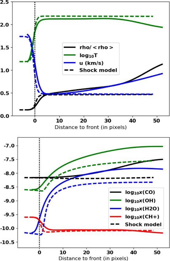
Molecular excitation in decaying turbulence                               821

                                                                                                                                                                     Downloaded from https://academic.oup.com/mnras/article/495/1/816/5841083 by guest on 20 September 2020
Figure 4. Time evolution of some heating and cooling rates. The viscous
                                                                                  Figure 5. Time evolution of the average abundance relative to nH for some
heating is computed only at times for which the maps of all relevant variables
                                                                                  relevant species. Also indicated is the population of the level v = 0, J = 3
(ρ, u, p) were retained. The kinetic energy decrease rate is computed
                                                                                  of H2 , scaled down by a factor of 1000 to help readability. Reference times
from finite difference on the kinetic energy data of Fig. 3 (solid line) or
                                                                                  are indicated as in Fig. 1 (note that the time axis is now logarithmically
from individual snapshots where the dissipative heating and compressive
                                                                                  scaled).
heating are integrated over the computational box and added together (open
circles). The photoelectric heating rate (dash-dotted line) and the cooling
from spontaneous de-excitation from H2 levels (dotted) are also indicated.
Reference times are indicated as in Fig. 1.

estimated from the average populations of the H2 levels,
                 J =6

    H2       =          AJ nJ (H2 ) EJ ,                                (3)
                 J =2

where AJ is the Einstein de-excitation coefficient of the Jth rotational
level. Fig. 4 shows that although H2 cooling reacts immediately
to the initial conditions, it takes a long time to relax back to
its original value. The rate of photoelectric heating is  photel =
4 × 10⁻²⁶ nH exp (− 2.5Av0 ) erg cm–3 s−1 (Black & van Dishoeck
1987). Because the visual extinction Av0 = 0.1 mag is assumed to be
a uniform constant and mass is conserved, the average photoelectric
heating rate is constant over time. Although this heating rate begins
to dominate over the average dissipative heating at around t =
3000 yr, the average temperature at this point, and even beyond, is               Figure 6. Box-averaged H2 excitation diagrams at various epochs, showing
still significantly above its initial radiative equilibrium (see Fig. 1).         log10 NJ /gJ , where NJ is the total column density (in cm−2 ) of level J across
This is a manifestation of the intermittency of the dissipative rate,             the box and gJ is its statistical weight. The black dashed line shows numbers
which peaks at values much larger than its average, and of the                    for a line of sight through the galaxy, as observed by Falgarone et al. (2005).
thermal inertia of the gas, which takes time to cool down after a                 Column densities are taken from their table 2, divided by a factor of 104 to
burst of heating.                                                                 account for the fact that their line of sight has a total column density of the
                                                                                  order of NH = 1022 cm−2 while our simulation only has NH = 1018 cm−2 .

3.1.2 Average abundances                                                          the chemical yields, which illustrates one possible observational
                                                                                  signature of turbulent dissipation. Fig. 6 shows the evolution of the
Fig. 5 shows the time evolution of the average abundances of                      H2 excitation diagram averaged over the computational domain.
selected molecules. Molecular chemistry is clearly boosted for a                  H2 levels above J = 3 are quickly excited and reach a maximum
significant amount of time, and it then decays back to the initial                between t = 200 yr and t = 300 yr, depending on which level
chemical equilibrium. For example, the abundance of CO is en-                     is considered, shortly after the maximum of the temperature (see
hanced by a factor of 10 and survives during a few thousand yr after              Fig. 1). However, level J = 2 reaches its maximum around t =
the initial kinetic energy burst. By contrast, the abundance of the               1000 yr. Excited populations are maintained, despite the fact that
H+3 cation is enhanced by a factor of 2. In Section 3.4.2, we discuss             the average temperature decreases again to values close to the initial
possible mechanisms that can enhance molecular production.                        state. The excitation of the lowest energy levels decays slower than
                                                                                  for higher energy levels, in agreement with the increase of Einstein
                                                                                  coefficients with the energy of the level: indeed, 1/Aij = 1000 yr
3.1.3 H2 excitation
                                                                                  for J = 2 while its value is 1 yr for J = 6. The slow variation of
Fig. 5 also shows that the upper-level population of the H2 0–0S(1)               H2 excitation justifies the use of a time-dependent treatment for
transition is boosted by a factor of nearly 2000, in conjunction with             populations of its excited levels. The ortho-to-para ratio is virtually

                                                                                                                             MNRAS 495, 816–834 (2020)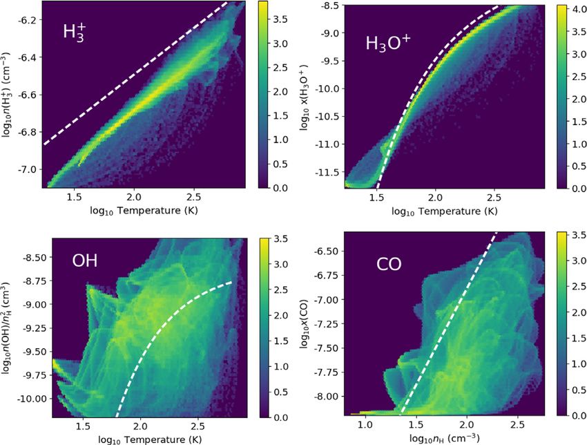
822          P. Lesaffre et al.
constant throughout the simulation (its value is about 0.67 initially
and increases to 0.71 at the end of the simulation).
   The black dashed line in Fig. 6 shows observational results from
Falgarone et al. (2005) for a line of sight throughout our Galaxy
selected to intercept mainly diffuse gas. We scale down the observed
column densities by a factor of 104 to account for the reduced
total column density in our simulation (NH = 1018 cm−2 across our
simulation, while it is estimated to be of the order of 1022 cm−2 in
the observed line of sight). Both the absolute value and the slope
of the resulting excitation diagram appear roughly consistent with
the early stages of the simulation, between t = 100 yr and t =
300 yr. The slope in the observations is slightly shallower than in
our simulations, hinting at the presence of gas with even larger

                                                                                                                                                               Downloaded from https://academic.oup.com/mnras/article/495/1/816/5841083 by guest on 20 September 2020
temperatures in the line of sight. Current and future observations
by the Stratospheric Observatory for Infrared Astronomy (SOFIA),
the James Webb Space Telescope (JWST) and the Space Infrared
Telescope for Cosmology and Astrophysics (SPICA) will require
and allow more precise and detailed comparisons.

3.2 Velocity field
In three-dimensional (3D) compressible experiments of solenoidal
driving for turbulence, it is customary to show the spectra of ρ 1/3 u,
rather than those of kinetic energy (ρu2 ) or velocity (u), because they
exhibit Kolmogorov-like (k−5/3 ) scaling (Federrath 2013). Fig. 7
shows spectra of ρ 1/3 u for three selected times of the simulation.
Energy always decreases with time. These spectra display a power-
law behaviour for about a decade, close to k−3 , but their slope
slowly drifts to steeper values as time proceeds. These power laws
experience an exponential cut-off at small scales due to viscous
dissipation and the cut-off scale appears to grow with time. We
computed the cross-scale flux (k) as in Grete et al. (2017), which
positive sign indicates that the net cascade of kinetic energy is
                                                                              Figure 7. Top: time evolution of the spectra of ρ 1/3 u (dimensionless units).
direct, from large to small scales (see Fig. 7). We followed Grete            Bottom: energy flux across wavelength k: (k) = TU U a + TU U c + TP U
et al. (2017) to decompose this energy flux across scales according           (black) and its components (blue, advection TU U a ; yellow, compression
to the sum of three different physical contributions. The energy flux         TU U c ; green, pressure TP U ; see text and Grete et al. 2017) at t = 300 yr.
due to advection TU U a (defined in Grete et al. 2017, equation 25) is
positive, while the fluxes due to compression TU U c (see Grete et al.
2017, equation 25) and pressure terms TP U (see Grete et al. 2017,            dissipation occurs in ridges with slightly fewer than 10 pixels (∼6
equation 32) are negative.                                                    au) of width, while vortical dissipation trails these compressive
                                                                              fronts.
3.3 Dissipation field                                                            Indeed, vorticity is known to be generated at shock crossings
                                                                              or at strong shock-front bends. The compressive heating fraction
We study the dissipation term       viscous .   When μ = ρν is a uniform      strongly decreases over time: from 80 per cent at the beginning
constant, we can write                                                        to about 8 per cent at the end of the simulation (not shown here).
                                                                            The statistics of viscous dissipation roughly display a lognormal
 viscous  = comp + sol ,                                             (4)
                                                                              behaviour (see Fig. 9), which is a signature of its intermittency
where the compressive dissipation is                                          (Kolmogorov 1962).
         4
 comp   =  ρν (∇ · u)2                                                 (5)
         3
and the vortical (or solenoidal) dissipation is                               3.4 Spatial distributions

 sol   = ρν (∇ · u)2 .                                                 (6)    3.4.1 Temperature and density
   However, equality (4) only holds averaged over the computational           Heating and compression in the wake of strong dissipation regions
domain, and we use ν as a uniform constant, not μ. This means,                hint at shocks (see Fig. 10). An inspection by eye of the pressure field
in our case, that the quantity defect ≡ viscous − comp − sol can be           frame by frame (one frame every 109 s, or about 30 yr) reveals the
non-zero both locally and globally. Nevertheless, Fig. 8 shows that           shocks as pressure steps and allows us to witness their progression
 defect generally remains small: this colour map shows essentially            (see Fig. 11). Shocks are already formed from the second frame and
blue ( comp ) and green ( sol ), almost no red (| defect |), and the global   they appear in pairs, back to back. Around t = 200 yr, the first shock
average of | defect | amounts to less than 10 per cent of the total           crossings occur, and start generating secondary shocks and trailing
dissipation rate at worst. The same figure shows that compressive             vorticity.

MNRAS 495, 816–834 (2020)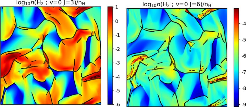
Molecular excitation in decaying turbulence                          823

                                                                                                                                                                 Downloaded from https://academic.oup.com/mnras/article/495/1/816/5841083 by guest on 20 September 2020
Figure 8. Map of the different components of the dissipation heating near
the peak of dissipation at t = 300 yr. The RGB colours of each pixel
are proportional to: blue, compressive heating comp ; green, solenoidal
heating sol ; red, remainder | defect |; while the intensity is proportional to
the logarithm of their sum. The pixels of lowest dissipation are masked out
(under a threshold such that their total dissipation amounts to 3 per cent of
the total dissipation).

                                                                                     Figure 11. Snaphots of pressure maps in the simulation at selected times.

                                                                                    3.4.2 Chemical analysis
                                                                                    We saw in Section 3.1.2 that the abundance of the H+      3 cation
                                                                                    is only mildly enhanced throughout our numerical experiment.
                                                                                    Indeed, its chemistry results from the balance between cosmic
                                                                                    ray ionization and dissociative recombination: its abundance is
                                                                                    insensitive to density,
                                                                                                   √        and mildly favoured by temperature increase
                                                                                    through the 1/ T dependence of the recombination rate of H+    3 . If
                                                                                    we write the balance between recombination and hydrogen cosmic
                                                                                    ray ionization, we can estimate its abundance as
                                                                                                                      0.5
                                                                                               ζ x(H2 )        T
                                                                                    n(H+
                                                                                       3) =                                 ,                              (7)
                                                                                               R0 x(C+ )     300 K
                                                                                    where R0 = 1.5 × 10⁻⁷ cm−3 s−1 is the H+      3 recombination rate at
Figure 9. Probability distribution function of the viscous dissipation   viscous
                                                                                    T = 300 K. We define n(S) as the abundance and x(S) = n(S)/nH as
at three selected epochs.                                                           the relative abundance of species S, and we have assumed that the
                                                                                    ionization degree is given by the abundance of C+ , the main carrier
                                                                                    of charges here. The relative abundance of H2 is quite uniform, and
                                                                                    equal to x(H2 ) = 0.4. In our simulations, the correlation between the
                                                                                    abundance of the H+  3 cation and the
                                                                                                                       √ temperature is remarkable and
                                                                                    displays the expected scaling in T (see Fig. 12, top-left panel).
                                                                                    The constant ratio of 70 per cent between the simulation results and
                                                                                    the dashed line still eludes us.
                                                                                       The temperature in this simulation is not large enough to over-
                                                                                    come the temperature activation barrier of 3000 K of the hydrogena-
                                                                                    tion reaction H2 + O → OH + H, as in the shocks of Lesaffre et al.

Figure 10. Temperature (left panel, linear scale) and density (right panel,
                                                                                                                                MNRAS 495, 816–834 (2020)
log scale) maps at t = 300 yr. Thin black contours of strong dissipation
(mean plus two standard deviations of log ) are overlaid to guide the eye.
824         P. Lesaffre et al.

                                                                                                                                                                Downloaded from https://academic.oup.com/mnras/article/495/1/816/5841083 by guest on 20 September 2020
Figure 12. Joint distribution between various abundances and temperature
or density with predictions from chemical balance (white dashed lines) for
H3 + at top left (equation 7), H3 O+ at top right (equation 8), OH at bottom left
(equation 9) and CO at bottom right (equation 10, without the exponential           Figure 13. Relative abundance maps at t = 300 yr for a choice of species.
temperature dependence). The colour scale indicates the decimal logarithm           Thin black contours of strong dissipation are overlaid.
of the number of pixels in the simulation that fall in each hexagonal bin.
These distributions are shown for time t = 300 yr.                                  left panel), the OH abundance above the dashed line is a footprint
                                                                                    of a previous episode of stronger heating or compression.
(2013). However, it helps to trigger the charge exchange reaction                      CO results from ion-neutral reaction OH + C+ (with rate R3 =
H+ + O → O+ + H, which has a much milder threshold of 227 K.                        1.6 × 10⁻⁹ cm3 s−1 ) followed by hydrogenation to give HCO+ ,
The hydrogenation reaction chain can then proceed from O+ until                     whose dissociative recombination yields CO. If we assume that
H3 O+ , which recombines to give either H2 O (branching 1/3) or OH                  these three reactions are fast, we can use equation (9) to compute
(branching 2/3). The hydrogenation chain is so efficient that the                   the rate of reaction of OH with C+ and balance it against the
relative abundance of H3 O+ can be obtained quite accurately from                   photodissociation rate of CO (about G0 × 3.5 × 10−11 s−1 in the
the balance between the rate of H+ + O → O+ + H with rate R1 =                      irradiation conditions of our simulation):
6 × 10⁻¹⁰ e−227 K/T cm3 s−1 and the rate of recombination of H3 O+                                2 x(H+ )x(O)x(C+ ) −227 K/T
with rate R2 = 1.2 × 10⁻⁶ (T/300 K)−0.5 cm3 s−1 ,                                   x(CO) = n2H                     e         90 cm6 .                  (10)
                                                                                                  3        G20
                           x(O)x(H+ )                                               Here, it can be seen that the effect of compression (nH ) is even more
x(H3 O+ ) = 5 × 10⁻⁴                  (T /300 K)0.5 e−227 K/T ,              (8)
                             x(C+ )                                                 important than for OH. This is because higher density helps against
as illustrated by Fig. 12 (top-right panel). The abundances relative                photodissociation of both OH and CO. However, the match with
to nH of atomic O, C+ ion and proton H+ are remarkably homoge-                      the simulation is now much worse, although the scaling with n2H is
neous: x(O) = 3 × 10⁻⁴ , x(C+ ) = 1.4 × 10⁻⁴ (all C is photoionized                 roughly visible; see Fig. 12 (bottom-right panel), where the white
at G0 = 1) and x(H+ ) = 5 × 10⁻⁶ result from the balance between                    dashed line represents equation (10) without the exponential tem-
cosmic ray ionization and H+ recombination.                                         perature dependence. Indeed, equation (10) assumes equilibrium,
   Similarly, it is expected that the abundance of OH results from                  which is even harder to realize due to the long photodissociation
the balance between the recombination of H3 O+ (with branching                      time-scale of CO (900 yr; i.e. comparable to the large-scale turnover
ratio 2/3 towards OH, the other 1/3 going to H2 O) and the                          time).
photodissociation of OH, with rate R3 = 2.9 × 10⁻¹⁰ G0 e−1.7Av0                        Surprisingly, CH+ is also among the molecules whose total
s−1 :                                                                               abundance is significantly enhanced (by a factor of 10, although
                                                                                    for about 100 yr of time only; see Fig. 5), despite our neglect of
x(OH)  2    x(O)x(H+ ) −227K/T −3                                                   ambipolar drifts. We show in Section 3.4.5 how this is linked to the
      = 2.0           e       cm .                                           (9)
  nH   3       G0                                                                   excitation of H2 levels.
The agreement between this prediction and the situation in the
simulation (see Fig. 12, bottom-left panel) is not as good as for
                                                                                    3.4.3 Abundance maps
H3 O+ because the destruction rate of OH is a slow process and its
abundance is not at chemical equilibrium. Note that in equation (9)                 Molecular production seems to be located in the wake of the strong
we took care to separate on the right-hand side the temperature                     dissipation regions (see Fig. 13). CO, OH (not shown, but similar to
contribution (from the threshold effect of the charge exchange                      CO) and H2 O can be locally enhanced by three to almost five orders
reaction H+ + O → O+ + H) and on the left-hand side the                             of magnitude. This is due both to the temperature threshold effect for
density contribution (from two-body formation reactions versus                      the charge exchange reaction O + H+ and to the compression effect,
photoreactions). A shock can contribute through the surge of heat                   which protects molecules against photodissociation as discussed
due to the dissipation, or through the compression that persists                    above, and so CO, OH and H2 O have similar maps. By contrast,
further away in the wake of the shock. A shearing sheet would                       H+3 is more mildly tied to the temperature, and so shows less
contribute only through the temperature surge. In Fig. 12 (bottom-                  marked variations. Finally, CH+ is strongly enhanced only in the

MNRAS 495, 816–834 (2020)
Molecular excitation in decaying turbulence                       825
                                                                                slowly to their multiphase condensation and evaporation history
                                                                                or to their alternating shielded and irradiated periods. This could
                                                                                explain the presence of warm H2 susceptible to produce CH+ at the
                                                                                edge of clumps (see Valdivia et al. 2017). Agúndez et al. (2010)
                                                                                and Zanchet et al. (2013) suggested that H2 excitation can help skirt
                                                                                the formation threshold, and thus play a role in CH+ formation. We
                                                                                show below in this subsection that this is the mechanism at play in
                                                                                the present work.
                                                                                   Dove & Mandy (1986) formulate a method to compute the state-
                                                                                to-state rates of endoergic reactions with excited H2 , using state-
                                                                                to-state thresholds lowered by the excitation energy of the H2 level
Figure 14. Map of the relative abundance (log scale) of the upper level of      considered: they use this formalism for H2 collisional dissociation.
H2 S(1) (J = 3, left panel) and the level J = 6 (right panel) at t = 300 yr.    Lesaffre et al. (2013) implement this method in the Paris–Durham

                                                                                                                                                          Downloaded from https://academic.oup.com/mnras/article/495/1/816/5841083 by guest on 20 September 2020
Thin black contours of strong dissipation are overlaid. The maxima of the
                                                                                shock code for the C+ + H2 → CH+ + H reaction. We use the same
level J = 6 often coincide with the peaks of CH+ abundance (marked on the
                                                                                implementation here, which follows the prescription by Agúndez
right panel as grey dashed contours where n(CH+ )/nH = 10−6.5 ).
                                                                                et al. (2010).
hottest regions, which suggests a sharp temperature threshold effect,              In the present simulation at age 300 yr, CH+ formation coincides
although the temperature threshold for its formation reaction C+ +              exactly with places where the J = 6 level has a high abundance (see
H2 → CH+ + H2 is 4600 K, way above the maximum temperature                      Fig. 14). This level has an energy of E6 /k = 3470 K, which closes
of the simulation at that time (around 850 K). We show that this is             a good fraction of the energy gap of 4300 K necessary to produce
linked with the H2 excitation in Section 3.4.5.                                 CH+ : even a mild temperature of 800 K can alleviate the threshold
                                                                                from this level. On average, over the computational domain at t =
                                                                                300 yr, 90 per cent of the formation rate of CH+ comes from the
3.4.4 H2 excitation                                                             J = 6 level. The average rate of formation for the C+ + H2 →
                                                                                CH+ + H reaction is increased by more than 200 times compared
Strong excitation of H2 takes place in the wake of strong dissipation           with what the Hierl, Morris & Viggano (1997) rate would give and
regions (see Fig. 14). In particular, the third rotational level of H2 can      by a factor of 1300 when compared with the Gerlich et al. (1987)
be locally enhanced by nearly seven orders of magnitude compared                rate. This raises the question of whether we should employ the same
with its value in the initial conditions: this should produce huge              state-to-state rates for other endoergic reactions such as the O + H2
contrasts in the emmissivity of the 0–0S(1) line of H2 . However,               → OH + H reaction, which is subject to a 3000 K temperature
the ortho-to-para ratio is almost homogeneous (not shown): the                  threshold and could well benefit similarly from H2 excitation. It
conversion of ortho to para states is very slow compared with the               would then pave the way to enhance even more the production of
thermalization of excited levels within even and odd states. The                other molecules such as H2 O or CO. This calls for the necessity
ortho-to-para thermalization occurs on much longer time-scales                  of computing such state-to-state rates, with all the complexity this
than the dynamical times in the simulation. The smaller range                   implies.
of variation of the higher-energy levels gives some a posteriori
justification for the use of a maximum rotational number Jmax = 6.
                                                                                4 T H E RO L E O F S H O C K S
                                                                                The above exploration suggests that molecule production, excita-
3.4.5 CH+ formation
                                                                                tion, compression and heating are tied to dissipation. In this section,
Shortly after the surprising detection of large abundances of CH+               we draw a more detailed link between dissipation, chemistry and
in the ISM (Douglas & Herzberg 1941), there were a number of                    the shock fronts in the simulation.
tentative explanations to explain the boost of endoergic routes
of formation for CH+ . Elitzur & Watson (1978) proved that
                                                                                4.1 Shock front extraction procedure
shock heating could overcome the temperature threshold of the
C+ + H2 reaction to produce CH+ , but their models produced                     We select three epochs where we carefully examine the dynamical
copious amounts of OH as well, which was not observed. Draine &                 fields and try to interpret them as a collection of shocks: epoch I
Katz (1986) and Pineau des Forêts et al. (1986) then showed how                (t = 300 yr), epoch II (t = 1100 yr) and epoch III (t = 3000 yr) .
ion-neutral reactions could be enhanced by the ion-neutral drift                   We first find the ridges of strong dissipation by applying DIS-
due to ambipolar diffusion in C-type shocks, with the result of                 PERSE (Sousbie 2011) to the dissipation field. This algorithm detects
producing CH+ with temperatures below the activation barrier for                the spines of the ridges as a list of pixel vertices, which makes it
OH formation. Falgarone et al. (1995) and Joulain et al. (1998)                 cumbersome to define the local direction of the filament’s spine.
have shown how incompressible dissipation bursts can provide                    Hence, we smooth each filament identified by DISPERSE using
the necessary heat to generate molecules. Godard et al. (2009)                  cubic B-splines with a smoothing condition of a width of 5 pixels
and Godard, Falgarone & Pineau des Forêts (2014) later included                (scipy.interpolate.splprep implementation of Dierckx 1982). The
the effect of the ion-neutral drift, which helps to enhance CH+                 smoothed filaments are overlaid on the dissipation field in Fig. 15.
with respect to OH, as required by observations. Lesaffre et al.                Even though the algorithm does a good job even in crowded hubs,
(2007) suggested that contact between the atomic warm neutral                   we note the detection is not completely exhaustive, as many endings
medium and the cold molecular interiors of diffuse clouds could                 are missed.
help gather C+ and H2 in an environment sufficiently warm to                       We then parse each filament along its length: every 10 pixels,
trigger the formation route of CH+ at the cloud interfaces. Valdivia            we compute tangential and normal unit vectors to the filament. We
et al. (2016) proposed that H2 chemistry of fluid parcels adapts too            inspect the dissipation field along the normal vector to find the pixel

                                                                                                                      MNRAS 495, 816–834 (2020)
826 P. Lesaffre et al.
this position if it lies closer than to an edge of the domain, to avoid
issues with its periodicity.
We make a first guess for the shock entrance velocity u0 in its
steady-state frame, by using
ρ()un () − ρ(−)un (−)
u0 = , (11)
ρ() − ρ(−)
which comes from the requirement of mass conservation in the
steady-state shock frame; note that Rankine–Hugoniot requires ρ(u
− u0 ) to be constant. We use this first-guess velocity to transform
the velocity un to a shock frame velocity and to estimate steady-
state frame mass, momentum and energy fluxes Ṁ, Q̇ and Ė
Downloaded from https://academic.oup.com/mnras/article/495/1/816/5841083 by guest on 20 September 2020
(Appendix A2) along with the constant transverse velocity ut0 .
We finally adjust the five parameters u0 , ut0 , Ṁ, Q̇ and Ė in the
analytical solution of Appendix A2 starting from these first-guess
estimates until the minimum of the sum of the normalized profile
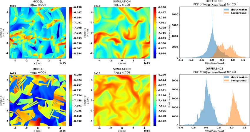
Figure 15. Smoothed DISPERSE dissipation filaments (dotted lines) over- averaged square residuals of ρ, un , ut , p and is reached. In other
laid on the dissipation field (log scale of the rate in erg cm−3 s−1 ) at time words, we minimize the dimensionless residual,
t = 300 yr.
y − yanalytics 2
r =
2
, (12)
y∈{ρ,u ,u ,p, }
yref
n t profile
which should be small when the analytical model is a good
representation of the simulation profile. The reference values to
normalize these quantities are defined as their maximum values
within a distance to the maximum dissipation position (the domain
where we restrict the shock profile adjustment). Note that we do not
fit for the viscous coefficient, as we keep it fixed to the input value
used in the hydrodynamic computation; we have shown that the
resolution is high enough so that the extra viscosity due to the
numerical scheme is negligible. Because the resulting residuals r2
we achieve are typically well below 1 (median 6 × 10⁻³ , best value
3 × 10⁻⁴ for epoch I on the selected shocks), we are confident that
this is indeed the case. A typical example is illustrated in Fig. 16.
When the residual r2 is below 0.1, and the shock entrance velocity
Figure 16. A typical (r2 = 0.0058) shock adjustment at epoch I. The five is above the speed of sound, we identify this point as a shock
quantities ln (log of dissipation, blue), ρ (mass density, red), p (pressure, and record its parameters. Fig. 17 displays all shocks fulfilling
green), un (normal velocity, cyan) and ut (tangential velocity, magenta) that
these conditions as black arrows proportional to the shock entrance
take part in the fit are displayed, normalized by their relevant scales so
velocity overlaid on the dissipation field.
that their contribution to the residuals is directly visible. Solid lines are
the profiles interpolated in the simulation, dashed lines are the best-fitting We used the method SHOCK FIND as described in Lehmann,
analytical model from Appendix A2. Vertical dotted lines indicate the region Federrath & Wardle (2016) to extract shock parameters and compare
of the fit and the position of the shock (s = −, 0, +), labelled in pixels. them with our current method. For each shock position found in our
The black dots illustrate the parabolic adjustment of the log of dissipation, simulation, we use the local direction of the shock (as opposed
which we use to find the origin of the profile and the curvature radius . to the density gradient proposed by the SHOCK FIND method)
The adjusted shock model has speed 1.34 km s−1 (Mach number 1.76) and and we define the pre-shock density and shock velocity as in steps
entrance density nH = 65 cm−3 . (iv) and (v) of Lehmann et al. (2016). We use Npix = 6, which
means pre- and post-shock values are taken 3 pixels before and after
where the maximum of the dissipation lies and we set this point as the maximum of dissipation. We compare the resulting entrance
the origin of distances along the normal (see Fig. 16). We find in velocity and density for our shocks in Fig. 18. The agreement for
which direction the density field grows, and we set this direction as the entrance density is good, with a small scatter. However, there
a positive coordinate along the normal. We now interpolate all fields is a larger scatter for the velocity, and there seems to be a small
along this direction with a sampling rate of a fifth of a pixel to build bias between both our methods, with SHOCK FIND finding larger
a 1D profile of every relevant dynamical variable: mass density values at larger velocities, and smaller values at lower velocities.
ρ, perpendicular (along the normal) un and transverse (along the In particular, SHOCK FIND finds Mach numbers slightly below 1
tangent) ut velocities, pressure p, and dissipation field . We fit a for most of the lowest velocity shocks (for which our method finds
parabola to the logarithm of the dissipation field to fine tune the values slightly above 1), and would not have labelled them as shocks.
position of the maximum dissipation, which we set as the new One dissipative structure is even detected by SHOCK FIND as a
origin of coordinates along the profile. We use this parabola to negative velocity shock, and inspection of the profile at this position
compute the curvature radius at maximum dissipation as −2 = shows that there is virtually no velocity jump, which puts the result
−(∂2 ln /∂s 2 ) = max (where s is the coordinate along the normal of our fit into question in this isolated case. The discrepancy at larger
to the filament; see the vertical dotted lines in Fig. 16). We discard velocity may introduce some bias in the statistical distribution of
MNRAS 495, 816–834 (2020)You can also read