Mapping rainfall hazard based on rain gauge data: an objective cross-validation framework for model selection - HESS
←
→
Page content transcription
If your browser does not render page correctly, please read the page content below
Hydrol. Earth Syst. Sci., 23, 829–849, 2019
https://doi.org/10.5194/hess-23-829-2019
© Author(s) 2019. This work is distributed under
the Creative Commons Attribution 4.0 License.

Mapping rainfall hazard based on rain gauge data: an objective
cross-validation framework for model selection
Juliette Blanchet1 , Emmanuel Paquet2 , Pradeebane Vaittinada Ayar1 , and David Penot2
1 Univ.  Grenoble Alpes, CNRS, IGE, 38000 Grenoble, France
2 EDF   – DTG, 21 Avenue de l’Europe, BP 41, 38040 Grenoble CEDEX 9, France

Correspondence: Juliette Blanchet (juliette.blanchet@univ-grenoble-alpes.fr)

Received: 1 March 2018 – Discussion started: 23 March 2018
Revised: 23 January 2019 – Accepted: 5 February 2019 – Published: 13 February 2019

Abstract. We propose an objective framework for selecting          an amount is expected to occur on average at this location. In
rainfall hazard mapping models in a region starting from rain      other words, it requires knowledge of the cumulative distri-
gauge data. Our methodology is based on the evaluation of          bution function (CDF) of extreme rainfall at any grid point
several goodness-of-fit scores at regional scale in a cross-       of the map. However, there are other situations when not
validation framework, allowing us to assess the goodness-          only the largest rainfalls are of interest, but also smaller and
of-fit of the rainfall cumulative distribution functions within    even zero rainfall values. This is for example the case in rain-
the region but with a particular focus on their tail. Cross-       fall simulation frameworks, e.g., when rainfalls are input of
validation is applied both to select the most appropriate sta-     spatially distributed hydrological models. In such a case one
tistical distribution at station locations and to validate the     needs to be able to simulate any possible rainfall field. This
mapping of these distributions. To illustrate the framework,       implies knowing both the local occurrence of any rainfall
we consider daily rainfall in the Ardèche catchment in the         value with the right frequency, and not only the largest ones,
south of France, a 2260 km2 catchment with strong inhomo-          and their spatial co-occurrence. Other domains include the
geneity in rainfall distribution. We compare several classical     evaluation of numerical weather simulations (e.g., Froidurot
marginal distributions that are possibly mixed over seasons        et al., 2018) or the investigation of the climatology of rainfall
and weather patterns to account for the variety of climato-        events in a region.
logical processes triggering precipitation, and several clas-         A difficulty in producing rainfall return level maps is that
sical mapping methods. Among those tested, results show a          knowing the CDF at any grid point ideally requires obser-
preference for a mixture of Gamma distribution over seasons        vation of rainfall on a grid scale. However, long-enough
and weather patterns, with parameters interpolated with thin       gridded data with good-enough quality are often lacking.
plate spline across the region.                                    Radar and satellite estimations are usually available for about
                                                                   10 years at best, and only for selected regions. In addi-
                                                                   tion, rainfall estimation in complex topography is particu-
                                                                   larly tricky, e.g., due to the mountain ranges shielding the
1   Introduction                                                   radar beam (Germann et al., 2006), or to the complex re-
                                                                   lationship between satellite-measured radiances and rainfall
In recent years, Mediterranean storms involving various spa-       reaching the ground (Tian and Peters-Lidard, 2010). On the
tial and temporal scales have hit many locations in south-         other hand, rain gauge networks are usually operational for
ern Europe, causing casualties and damages (Ramos et al.,          50 to 100 years in the main part of the world, at least at daily
2005; Ruin et al., 2008; Ceresetti et al., 2012a). Assessing       scale, but they only provide point observations. Thus, two
the frequency of occurrence of extreme rainfall in a region is     main methods are usually adopted for estimating the CDF of
usually done by the computation of return level maps. This         rainfall at any location when observations are only available
requires relating any (large) amount of rainfall at a given lo-    at selected locations. The first one resorts to the spatial inter-
cation to its return level, i.e., to the frequency at which such

Published by Copernicus Publications on behalf of the European Geosciences Union.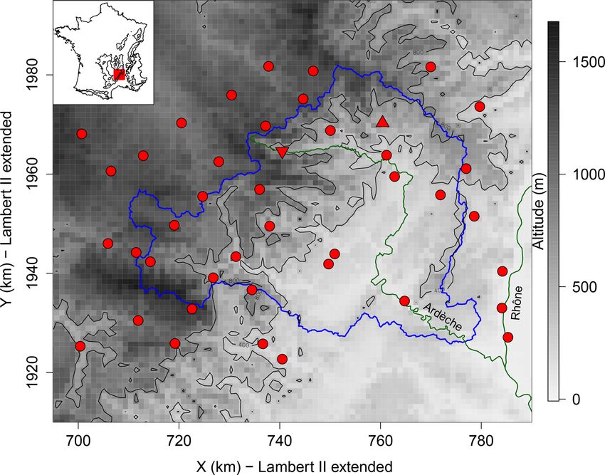
830                                                J. Blanchet et al.: Cross-validation framework for mapping rainfall hazard

polation of point data supplied by rain gauges. This allows           catchment in the south of France. Despite its relatively small
transformation of point observations into gridded ones, and           size, this test case is particularly challenging as it shows ex-
so estimation of gridded CDFs of rainfall. Among the best             traordinarily strong inhomogeneity in rainfall statistics at a
performing methods for spatial interpolation of daily rain-           very short distance. Following previous studies in the region
fall are kriging, inverse distance weighting and spline-surface       (Evin et al., 2016; Garavaglia et al., 2010, 2011; Gottardi
fitting (e.g., Camera et al., 2014; Creutin and Obled, 1982;          et al., 2012), the compared marginal distributions involve
Goovaerts, 2000; Ly et al., 2011; Rogelis and Werner, 2013).          seasonal and weather pattern subsampling, considering dif-
In complex topography, there may be some gain in applying             ferent models for the subclass-dependent distributions. How-
these methods locally, e.g., considering local precipitation al-      ever, the proposed cross-validation framework is general, as
titude gradients (Frei and Schär, 1998; Gottardi et al., 2012;        it involves objective criteria, and could likewise be used to
Lloyd, 2010). However, none of the above statistical methods          select among any other distribution. Section 2 presents the
is able to fully account for the statistical properties of rainfall   data. Sections 3.1 and 3.2 describe the marginal distributions
fields. A first difficulty is due to the presence of zeros, which     and mapping models considered in this study and present the
complicates interpolation and can lead to negative interpo-           cross-validation scores of model selection. Section 3.3 de-
lated rainfalls – although this could be partially overcome by        tails the procedure of model selection from marginal model-
using analytical transformation of the raw variable. A second         ing to hazard mapping. Section 4 gives extensive results for
difficulty is that rainfall distribution is usually heavy tailed,     the Ardèche catchment. Section 5 concludes the study.
and interpolation methods, by smoothing values, lack qual-
ity for representing the most extreme events (Delrieu et al.,
2014).                                                                2   Data
    A second way of mapping rainfall hazard is, rather than in-
terpolating the point observations, to map the parameters of          We illustrate our framework on the Ardèche catchment
CDFs fitted on rain gauge series. In addition to the choice of        (2260 km2 ) located in the south of France (see Fig. 1). The
interpolation models comes now the choice of the marginal             region includes part of the southeastern edge of the Mas-
model of rainfall amounts on wet days (referred to as nonzero         sif Central, where the highest peaks of the region are lo-
rainfalls). The most commonly used CDFs at daily scale in-            cated (more than 1500 m a.s.l), and the Rhône Valley (down
clude the exponential, Gamma, lognormal, Pareto, Weibull              to 10 m a.s.l). The southeastern slope of the Massif Central
and Kappa models (Papalexiou et al., 2013). Noting that               is known to experience most of the extreme storms and re-
these distributions tend to underestimate extreme rainfall            sulting flash floods (Fig. 2 of Nuissier et al., 2008). These
amounts (Katz et al., 2002), a recent flurry of research de-          so-called “Cévenol” events are produced by quasi-stationary
veloped hybrid models based on mixtures of distributions              mesoscale convective systems that stabilize over the region
for low and heavy amounts (Vrac and Naveau, 2007; Fur-                during several tens of hours. The positioning and stationar-
rer and Katz, 2008; Li et al., 2012). More recently Naveau            ity of these systems are largely influenced by the topography
et al. (2016) proposed a family of distributions that is able to      of the surrounding mountain massifs (Nuissier et al., 2008).
model the full spectrum of rainfall, while avoiding the use of        We use two daily rain gauge networks maintained, respec-
mixtures of distributions. Several studies compared marginal          tively, by Electricité de France and Météo-France. We con-
models for rainfall (e.g., Mielke and Johnson, 1974; Swift            sider the 15 rain gauges inside the catchment, together with
and Schreuder, 1981; Cho et al., 2004; Husak et al., 2007;            the 27 stations located less than 15 km outside. This gives a
Papalexiou et al., 2013), but focusing usually on a couple of         total of 42 stations with 20 to 64 years of data between 1 Jan-
CDFs. Other studies compared methods for mapping rainfall             uary 1948 and 31 December 2013. In both databases, daily
hazard, and particularly extreme rainfall, assuming a given           values are recorded every day at 06:00 UTC, corresponding
CDF (Beguería and Vicente-Serrano, 2006; Beguerïa et al.,             to rainfall accumulation between 06:00 UTC of the previous
2009; Szolgay et al., 2009; Blanchet and Lehning, 2010;               day and 06:00 UTC of the present day.
Ceresetti et al., 2012b). However, there is, to the best of              The Ardèche catchment is chosen for illustration purposes
our knowledge, no study assessing the goodness-of-fit of the          and because, despite its relatively small size, it shows strong
full procedure of rainfall hazard mapping, i.e., from marginal        inhomogeneity in rainfall distribution. To illustrate this, we
modeling to the production of hazard maps.                            show in Fig. 2 the averages of annual totals and annual max-
    Our study aims at filling this gap by proposing an ob-            imum daily rainfalls for each station. Computing the ratios
jective cross-validation framework that is able to validate           between the largest and lowest values in Fig. 2 gives ratios
the full procedure of rainfall hazard mapping starting from           of 2.6 for the annual totals and 3.2 for the annual maxima.
point observations. Our framework features three character-           For comparison the latter ratio is barely lower than the ra-
istics: (i) it selects both the marginal and mapping models,          tio found over the whole of France, which amounts to 4. For
(ii) it validates the full spectrum of rainfall, from short- to       both annual totals and annual maxima, the strongest values
long-term extrapolated amounts, and (iii) it applies on a re-         in the region are concentrated along the Massif Central ridge,
gional scale. The framework is illustrated on the Ardèche             while much smaller values are found a few kilometers apart

Hydrol. Earth Syst. Sci., 23, 829–849, 2019                                          www.hydrol-earth-syst-sci.net/23/829/2019/
J. Blanchet et al.: Cross-validation framework for mapping rainfall hazard                                                             831

Table 1. Considered models for the marginal distributions of nonzero rainfall. 0 in the Gamma density is the complete Gamma function
        ∞
0(κ) = r κ−1 e−r dr.
        R
         0

                   Distribution                     CDF G(r) or density g(r), for r > 0               Parameters

                                                    g(r) = r κ−1 e−r/λ / 0(κ)λκ

                   Gamma                                                                              λ > 0, κ > 0
                                                                       κ
                   Weibull                          G(r) = 1 − e−(r/λ)                                λ > 0, κ > 0
                                                              n                  o   √
                   Lognormal                        g(r) = exp −(log(r/λ))2 / 2κ 2 /(rκ 2π)           λ > 0, κ > 0
                                                                    κ
                   Extended exponential             G(r) = 1 − e−r/λ                                  λ > 0, κ > 0
                                                                              κ
                   Extended generalized Pareto      G(r) = 1 − (1 + ξ r/λ)−1/ξ                        λ > 0, κ > 0, ξ > 0

                                                                           0, we have the following decomposition:

                                                                           pr(R ≤ r) = p 0 + 1 − p 0 G(r),                              (1)

                                                                           where G is the CDF of nonzero rainfall at the considered sta-
                                                                           tion. Choice of G is an issue. One of the difficulties is that we
                                                                           wish to model adequately both the bulk of the distribution of
                                                                           nonzero rainfall and its tail, i.e., the probability of extreme
                                                                           rainfall occurring. The most common models for nonzero
                                                                           rainfall include the Gamma, Weibull and lognormal mod-
                                                                           els (Papalexiou et al., 2013), whose CDF G(r) or densities
                                                                           g(r) = ∂G(r)/∂r, r > 0 are given in Table 1. Although less
                                                                           common, another family of models for nonzero rainfall relies
                                                                           on univariate extreme value theory, which tells that probabil-
                                                                           ities of the form pr(R ≤ r|r > q), with q large, can be ap-
                                                                           proximated by either an exponential or a generalized Pareto
                                                                           tail (Coles, 2001, Sect. 4). This led Naveau et al. (2016) to
Figure 1. Region of analysis. The blue polygon is the Ardèche              propose the extended exponential and extended generalized
catchement. The red points show the locations of the stations. The
                                                                           Pareto distributions, whose CDF is given in Table 1. Note
upper triangle is station Antraigues and the lower triangle station
                                                                           that less parsimonious models are given in Naveau et al.
Mayres (both lie at about 500 m a.s.l.). The background shows the
altitude in gray scale (1 km raster cells). The top left insert shows      (2016), but they are not considered in the present study. The
a map of France with the studied region in red. The black lines are        extended exponential and extended generalized Pareto distri-
the 400 and 800 m a.s.l. isolines.                                         butions of Table 1 ensure that the occurrence probability of
                                                                           small (but nonzero) rainfall amounts is driven by κ, while the
                                                                           upper tail of nonzero rainfall is equivalent to a generalized
in the Massif Central plateau or in the Piémont. Concentra-                Pareto tail. The extended exponential model is also called
tion of daily rainfall and particularly of extreme daily rainfall          “generalized exponential” and has been used previously for
along the Massif Central ridge has already been documented                 extreme rainfall in Madi and Raqab (2007) and Kazmierczak
in many studies; see, e.g., Fig. 10 of Blanchet et al. (2016).             and Kotowski (2015).
We assume in this study temporal stationarity of rainfall. A                  In the models of Table 1, rainfall is implicitly assumed
case of potential nonstationarity due to climate change will               to come from a single distribution. This assumption may be
be discussed in Sect. 5.                                                   questioned. Indeed, different climatological processes trig-
                                                                           ger precipitation, leading to the occurrence of rainfall of dif-
                                                                           ferent natures and intensities (e.g., convective vs. stratiform
3     Method
                                                                           precipitation). Furthermore, rainfall occurrence and intensi-
3.1     Marginal distribution of rainfall                                  ties often vary with season, reflecting both variations in tem-
                                                                           perature and in storm tracks, for example. For this reason,
3.1.1    Considered marginal models                                        Garavaglia et al. (2010) proposed for the same region the use
                                                                           of subsampling based on seasons and weather patterns (WP)
Let R be the random variable of daily rainfall amount at a                 (see also Brigode et al., 2014; Blanchet et al., 2015, respec-
given station. R is zero with probability p 0 and, for any r >             tively, in Canada and Norway). Each day of the record period

www.hydrol-earth-syst-sci.net/23/829/2019/                                                 Hydrol. Earth Syst. Sci., 23, 829–849, 2019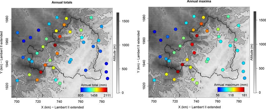
832                                                   J. Blanchet et al.: Cross-validation framework for mapping rainfall hazard

Figure 2. Panel (a): averages of annual totals (mm). Panel (b): averages of annual maximum daily rainfalls (mm).

is assigned to a WP. If S seasons and K WP are considered,
then days are classified into S × K subclasses. The law of                                                         K
                                                                                                                   X
                                                                                                                          00
total probability gives, for all r > 0,                                Gs (r) = pr(R ≤ r|R > 0, season = s) =            ps,k Gs,k (r),   (5)
                                                                                                                   k=1
              S X
              X K
pr(R ≤ r) =             pr(R ≤ r|season = s, WP = k)ps,k , (2)                                             K
                                                                              00 = p (1−p 0 )/(1−                      0 ). A similar idea
                                                                                                           P
                                                                       where ps,k   s,k  s,k                     ps,k ps,k
              s=1 k=1
                                                                                                           k=1
                                                                       is used in Wilks (1998) for example, but considering a mix-
where ps,k is the probability that a given day is in season s
                    PP                                                 ture of two (exponential) distributions in an unsupervised
and in WP k (thus       ps,k = 1). Following Eq. (1), R in
                         s k                                           way, i.e., without relying on a priori subsampling. It shows
                                            0 and, for any
season s and WP k is zero with probability ps,k                        the advantage of not requiring prior knowledge on the classi-
r > 0, we have the decomposition                                       fication, but it is at the same time more difficult to estimate,
                                                                     in particular if the models for different seasons and WP do
                                  0
pr(R ≤ r|season = s, WP = k) = ps,k + 1 − ps,k  0
                                                    Gs,k (r),          not differ much.
                                                                          In this article, we will consider the supervised case
where Gs,k is the CDF of nonzero rainfall at the considered            (Eq. 3), with S = 2 seasons and K = 3 WP, considering the
station for a day in season s and WP k. This gives in Eq. (2),         five models of Table 1 for the distribution of precipitation
for all r > 0,                                                         amounts Gs,k (see Sect. 3.3). This implies that estimation
                                                                       of Gs,k can be made independently of each others, by con-
                    S X
                    X K                                              sidering only the days of the record belonging to season s
pr(R ≤ r) = p 0 +                        0
                               ps,k 1 − ps,k   Gs,k (r),        (3)    and WP k. A variety of inference methods exists. For rainfall
                    s=1 k=1                                            analysis, two options are popular: maximum likelihood (ML)
              S P
                K                                                      estimation and a method of moments based on probability
where p 0 =
              P               0 is the probability of any day be-
                        ps,k ps,k                                      weighted moments (PWMs). However, as noted in Naveau
              s=1 k=1                                                  et al. (2016), ML estimation may fail for rainfall because the
ing dry. Nonzero precipitation amounts defined by Eq. (3)              discretization due to instrumental precision strongly affects
have CDF                                                               low values, which biases ML estimation if not accounted for.
                                S X
                                X K                                    One way to circumvent this issue is to resort to censored like-
                                            0                          lihood but choice of the censoring threshold is in itself an is-
G(r) = pr(R ≤ r|R > 0) =                   ps,k Gs,k (r),       (4)
                                 s=1 k=1                               sue. Results on our data (not shown) reveal that the threshold
                                                                       has to be no smaller than 5 mm. PWM, on the other side, is
         0 = p (1 − p 0 )/(1 − p 0 ). Equation (4) defines
where ps,k     s,k       s,k                                           much more robust against discretization since it is based on
a mixture of S × K distributions, e.g., a mixture of S × K             summary statistics, rather than on the exact values of obser-
Gamma distributions. Analogously, the CDF of nonzero pre-              vations (Naveau et al., 2016). For this reason, we estimate
cipitation amounts in a given season s is written as                   in this study the distributions of precipitation amounts Gs,k
                                                                       by PWM, while ps,k    0 at a given station is estimated empiri-

Hydrol. Earth Syst. Sci., 23, 829–849, 2019                                            www.hydrol-earth-syst-sci.net/23/829/2019/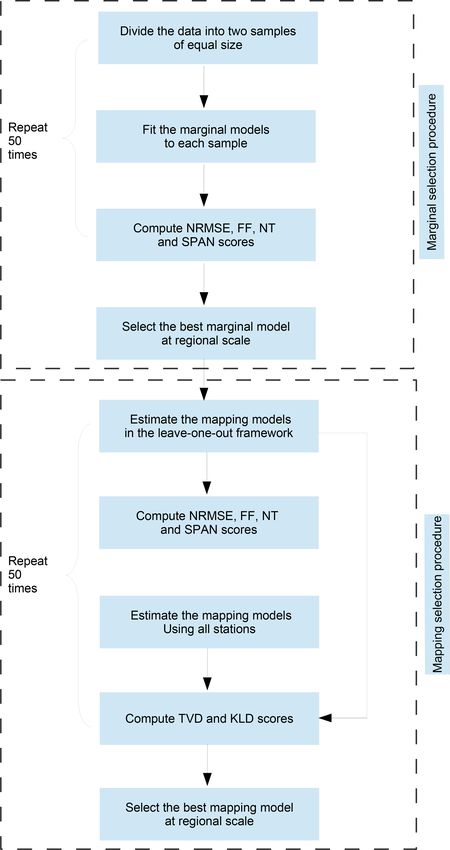
J. Blanchet et al.: Cross-validation framework for mapping rainfall hazard 833
Table 2. Summary of the considered scores for evaluating marginal and mapping models.
Score Assessment For which model?
NRMSE Accuracy of the whole distribution Marginal & mapping models
FF Reliability of the far tail Marginal & mapping models
NT Reliability of the close tail Marginal & mapping models
SPAN Stability at extrapolation Marginal & mapping models
TVD & KLD Spatial stability Mapping model
0 = d 0 /d where d is the number of observations
cally as p̂s,k symmetrically. Sc(11) and Sc(22) are calibration scores, while
s,k
0
and ds,k is the number of zero values in season s and WP k. Sc(12) and Sc(21) are cross-validation scores. For the sake of
Combining estimations in Eq. (3) gives an estimation of the conciseness, we detail below the case of Sc(12) for the differ-
rainfall CDF at the considered station, and in Eq. (4) an esti- ent scores.
mation of the CDF of nonzero rainfall. The NRMSE (normalized root mean squared error) evalu-
Estimates of return levels are then obtained as follows. The ates the reliability of the fits in the whole observed range of
T -year return level rT is the level expected to be exceeded nonzero rainfall, by comparing observed and predicted return
on average once every T years. It satisfies the relationship levels of daily rainfall. For a given station i ∈ {1, . . . , Q},
pr(R ≤ rT |R > 0) = 1−1/(T δ), where δ is the mean number (1)
1/2 , (1)
ni ni
of nonzero rainfall per year at the considered station. When (12)
1 X
(1) (2)
2 1 X (1)
subsampling Eq. (4) is considered, there is no explicit for- NRMSEi = r − r̂i,Tk ri,T , (6)
n(1) k=1 i,Tk (1)
n k=1 k
i i
mulation, and estimation of rT is obtained numerically by
solving pr(R ≤ rT |R > 0) = 1 − 1/(T δ) in Eq. (4). (1)
where ni is the number of nonzero rainfall in Ci for sta-
(1)
tion i, Tk ranges the observed return periods of nonzero rain-
3.1.2 Evaluation at regional scale in a cross-validation (1) (1)
fall in Ci , ri,Tk is the observed daily rainfall associated with
framework (1) (2)
the return period Tk for the subsample Ci and r̂i,Tk is the
(2)
The goal of this evaluation is to assess which marginal model Tk -year return period derived from the estimated Ĝi . With-
performs better at the regional scale, i.e., for a set of n sta- out loss of generality we assume T1 , . . . , Tn(1) to be sorted
i
tions taken as a whole, rather than individually. We follow the in descending order (so T1 is associated with the maximum
split sample evaluation proposed in Garavaglia et al. (2011) (1)
over Ci ). If station i has δi nonzero rainfall per year on
and Renard et al. (2013). We divide the data for each station i average, usual practice is to consider the kth largest return
(1) (2) (1) (1)
into two subsamples, Ci and Ci , and consider nonzero period as Tk = (ni + 1)/(δi k), k = 1, . . . , ni , and to esti-
rainfall for these two subsamples. We fit a given competing (1) (1)
mate ri,Tk as the kth largest observed rainfall over Ci . Esti-
model on each of the subsamples, giving two estimated dis- (2) (2)
(1) (1)
tributions of G in Eq. (4): Ĝi , estimated on Ci , and Ĝi ,
(2) mate r̂i,Tk is obtained numerically from Ĝi as described in
(2) (1)
estimated on Ci . Our goal is to test the consistency between Sect. 3.1.1. The normalization by the mean rainfall of Ci in
validation data and predictions of the estimates, both for the Eq. (6) allows comparison of NRMSE over stations with dif-
(12) (2)
core and tail of the distributions, and the stability of the es- ferent pluviometry. The smaller NRMSEi , the better Ĝi
(1)
timates when calibration data changes, focusing particularly fits the rainfalls over Ci . For the set of Q stations, we ob-
on the tail which is usually less stable. tain a vector of NRMSE(12) of length Q which should re-
As shown in Table 2, three families of scores are com- main reasonably close to zero. A regional score is obtained
puted, assessing, respectively, (i) accuracy of the estima- by computing the mean of the Q values:
tions along the full range of observations (MEAN(NRMSE)),
Q
(ii) reliability of the tail of the estimated distribution, check-
1 X (12)
MEAN NRMSE(12) = NRMSEi . (7)
ing in particular systematic over- or under-estimation of the Q i=1
observations (AREA(FF ) and AREA(NT )), and (iii) stabil-
ity of the tail at extrapolation (MEAN(SPAN)). The scores For competing models, the closer the mean is to 0, the better
relating the tail of the distribution have been proposed and the goodness-of-fit.
used in Garavaglia et al. (2011), Renard et al. (2013) and NRMSE assesses goodness-of fit of the whole distribu-
Blanchet et al. (2015). In the split sample evaluation frame- tion in the observed range. Now let us have a closer look
work, four scores can be derived of a given score Sc: Sc(12) is at the tail of the distribution, and in particular at the maxi-
(2) (1) (1)
the regional score when Gi is validated on the nonzero rain- mum over Ci ; i.e., at ri,T1 in Eq. (6), that for shortness we
(1) (1)
fall subsample Ci . Sc(21) , Sc(11) and Sc(22) are obtained denote mi . If Gi is the true distribution of nonzero rain-
www.hydrol-earth-syst-sci.net/23/829/2019/ Hydrol. Earth Syst. Sci., 23, 829–849, 2019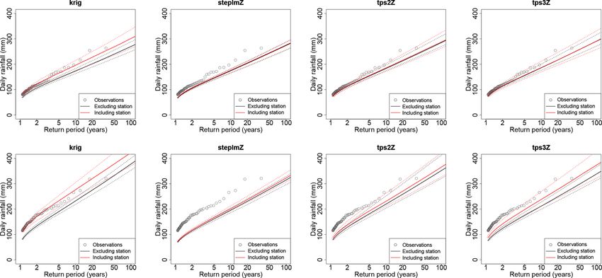
834                                               J. Blanchet et al.: Cross-validation framework for mapping rainfall hazard

Figure 3. Illustration of the FF score when the true CDF G0 is extended exponential with λ = 20 and κ = 0.3. The CDF G1 underesti-
mates G0 (λ = 25) while G2 overestimates G0 (λ = 15). (a) Histogram of {G0 (m)}n where m are 42 realizations of Gn0 and n = 4000.
(b) Histogram of {G1 (m)}n . (c) Histogram of {G2 (m)}n . The horizontal dashed lines show the uniform density on (0, 1).

                                                   (1)
fall, then the corresponding random variable Mi has distri-          histograms). By focusing of maximum values, the histogram
                           (1)
bution Gi to the power ni , whose variance is large. Thus            of ff (12) can be seen as a way of assessing systematic bias in
                                                    (1)              the far tail of the distribution. For a more quantitative assess-
computing error based on the single realization mi would
                                                                     ment, we compute the area between the density of the ff (12)
be very uncertain. For this reason, Renard et al. (2013) pro-
                                                                     and the uniform density as follows:
posed to make evaluation by pulling together the maxima
of the Q stations, after transformation to make them on the                             10
                                                                                   1 X      card (Bc )
same scale. It is based on the idea that if X has CDF F ,            AREA FF (12) =        10            −1 ,                       (8)
                                                                                    18 c=1        n
then F (X) follows the uniform distribution on (0, 1). Taking
         (1)               (1)                (2)                                                             (12)
X = Mi and F = (Gi )ni implies that, if Ĝi is a perfect             where card(Bc ) is the number of ffi           in the cth bin, for
estimate of Gi , then                                                c = 1, . . . , 10. The term inside the absolute value in Eq. (8) is
                          (1)
                                                                     the difference between densities in the cth bin. The division
   (12)       (2)   (1)
ffi       = {Ĝi (mi )}ni                                            by 18 forces the score to lie in the range (0, 1), with lower
                                                                     values indicating better fits (the worst case being all values
should be a realization of the uniform distribution. For the set     lying in the same bin). Figure 3 shows that, when Q = 42
of Q stations, this gives a uniform sample ff (12) of size Q.        stations are considered, a value of AREA(FF (12) ) around 0.2
Hypothesis testing for assessing the validity of the uniform         corresponds to no systematic bias in the very tail of the dis-
                                                (12)
assumption is challenging because the ffi            are not inde-   tribution at regional scale, whereas a value around 0.5 cor-
pendent from site to site, due to the spatial dependence be-         responds to a strong over- or under-estimation. In the latter
tween data. Thus Blanchet et al. (2015) proposed to base             case, only looking at the histogram can inform about whether
comparison on the divergence of the density of the ff (12) to        over- or under-estimation applies.
the uniform density. A reasonable estimate of the latter is ob-         The NT criterion is an alternative to FF assessing re-
tained by computing the empirical histogram of the ff (12)           liability of the fit of the tail but focusing on prescribed
with 10 equal bins between 0 and 1. As illustrated in Fig. 3,        (large) quantiles rather than on the overall maximum. It
      (2)
if Ĝi are good estimates of Gi , i = 1, . . . , Q, the histogram    applies the same principle as FF , involving a transforma-
of ff (12) should be reasonably uniform on (0, 1). If the his-                                                         (1)
                                                                     tion of X to F (X), but considering X as Ki,T , the random
                                (2)   (1)
togram is left-skewed, then Ĝi (mi ) tends to overestimate                                                              (1)
           (1)  (1)                                                  variable of the number of exceedances over Ci of the T -
the true Gi (mi ), or in other words the return period of the                                    (1)                (1)
                  (1)                                                year return level, i.e., Ki,T = card({Ri,j ∈ Ci ; Gi (Rj ) >
maximum over Ci tends to be underestimated (case of over-            1 − 1/(T δi )}), in which case F is the binomial distribu-
estimated risk). If the histogram is right-skewed, the return               (1)                       (1)                   (2)
                                                                     tion Bi with parameters (ni , 1/(T δi )). Thus, if Ĝi is
                                  (1)
period of the maximum over Ci tends to be over-estimated                                                 (12) (1) (12)
                                                                     a perfect estimate of Gi , then ni,T = Bi (ki,T ), where
(case of under-estimated risk). Although any scenario of mis-
                                                                                  n
fitting could theoretically be possible, in practice the his-          (12)                  (1)     (2)
                                                                     ki,T = card ri,j ∈ Ci ; Ĝi lef t (ri,j > 1 − 1/ (δi T )} ,
tograms of ff (12) show mainly the three above alternatives:
either a good fit (flat histogram), or a tendency towards a          should be a realization of the discrete uniform distribution.
                                                                                                    (12)
systematic under- or over-estimation (left- or right-skewed          Randomization to transform ni,T to a continuous uniform

Hydrol. Earth Syst. Sci., 23, 829–849, 2019                                          www.hydrol-earth-syst-sci.net/23/829/2019/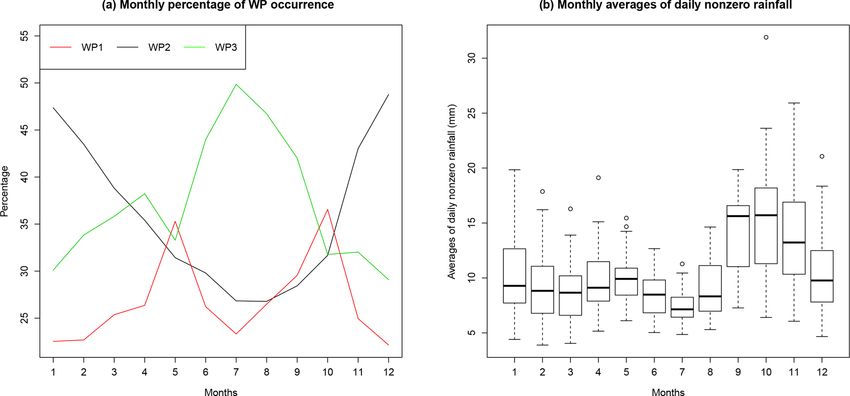
J. Blanchet et al.: Cross-validation framework for mapping rainfall hazard                                                                   835

variate on (0, 1) is proposed in Renard et al. (2013) and exten-     Table 3. Mapping models considered in this study, with involved
sively described in Blanchet et al. (2015). For i ranging over       coordinates. Kriging method provides exact interpolation, unlike
the set of Q stations, we thus obtain a sample of Q uniform          the linear regression and thin plate spline.
variates. Scores are calculated as for FF by comparing the
                           (12)                                       Name      Model                                    Coordinates   exact?
empirical densities of NT to the theoretical uniform den-
                                   (12)                               krig      Kriging without external drift           x, y          yes
sity, giving the scores AREA(NT ). Taking T as, e.g., half
                                                                      krigz     Kriging with external drift              x, y, z       yes
to one-quarter the length of the observations allows assess-          krigZ     Kriging with external drift              x, y, Z       yes
ment of the reliability of the close tail of the distribution. As
                                                                      steplmz   Stepwise linear regression               x, y, z       no
such, it is a good complement to FF that focuses on the far
                                                                      steplmZ   Stepwise linear regression               x, y, Z       no
tail (i.e., on the maximum).
   Last but not least, the SPAN criterion evaluates the stabil-       tps2      Bivariate thin plate spline              x, y          no
                                                                      tps2z     Bivariate thin plate spline with drift   x, y, z       no
ity of the return level estimation, when using data for each          tps2Z     Bivariate thin plate spline with drift   x, y, Z       no
of the two subsamples. More precisely, for a given return pe-         tps3z     Trivariate thin plate spline             x, y, z       no
riod T and station i,                                                 tps3Z     Trivariate thin plate spline             x, y, Z       no
                     (1)     (2)
                  |r̂i,T − r̂i,T |
SPANi,T =           n               o,                        (9)
                        (1)     (2)
                1/2 r̂i,T + r̂i,T                                    parameters for station i and θ̂i,j its j th element. θ̂i is com-
                                                                     posed of the S × K probability of zero rainfall ps,k    0 and the
          (1)
where r̂i,T ; e.g., is the T -year return level for the distribu-    2 × S × K or 3 × S × K parameters of the distributions Gs,k ,
                                         (1)
tion G estimated on subsample Ci of station i, i.e., such            depending on the marginal distribution (see Table 1). We as-
       (1) (1)
that Ĝi {r̂i,T } = 1 − 1/(T δi ). SPANi,T is the relative abso-     sume the θi,j ordered so that the first S × K elements are
                                                                            0 . We aim at estimating the surface response θ (l)
                                                                     the ps,k
lute difference in T -year return levels estimated on the two                                                                       j
subsamples. It ranges between 0 and 2; the closer to 0, the          at any l of the region, knowing θj (li ) = θ̂i,j . In this study
more stable the estimations for station i. For the set of Q sta-     we consider three of the most popular method: kriging in-
tions, we obtain a vector of SPANT of length Q with a dis-           terpolation, linear regression methods and thin plate spline
tribution which should remain reasonably close to zero. A            regressions. However, the parameters θj s are constrained,
rough summary of this information is obtained by comput-             whereas these models apply the unbounded variables: the
                                                                                      0 lie in (0, 1), while the parameters of Ta-
                                                                     probabilities ps,k
ing the mean of the Q values of SPANi,T , i = 1, . . . , Q:
                                                                     ble 1 are all positive. Therefore we apply the mapping mod-
                              Q
                           1 X                                       els to transformations of θj , i.e., to ψj = transf(θj ), where
MEAN (SPANT ) =                  SPANi,T .                   (10)
                           Q i=1                                     “transf” maps the range of values of θj to (−∞, +∞). In
                                                                     this study we consider ψj (l) = 8{θj (l)} if j ≤ S × K (i.e., if
For competing models, the closer the mean is to 0, the more                      0 ), where 8 is the standard Gaussian CDF, and to
                                                                     θj is any ps,k
stable the model is. When T is larger than the observed              ψj (l) = log{θj (l)} otherwise. Other transformations would
range of return periods, MEAN(SPANT ) evaluates the sta-             be possible, in particular ps,k0 may be transformed with the
bility of the return levels in extrapolation. Note that it is by     logit function, but will not be considered here for the sake
definition 0 in calibration, and thus it is only useful in cross-    of concision. Thus we aim at estimating ψ        ej (l) given val-
validation.
                                                                     ues ψj (li ) = ψ̂i,j at station locations, with obvious nota-
   For the sake of concision, in the rest of this article
                                                                     tions. If l ≤ S × K, estimates of θj (l) are then obtained as
the scores MEAN(NRMSE), AREA(FF ), AREA(NT ) and
                                                                     θj (l) = 8−1 (ψ
                                                                     e               ej (l)). Otherwise surface response estimates
MEAN(SPANT ) will be referred to as the NRMSE, FF , NT
                                                                     are obtained as e  θj (l) = exp(ψej (l)). For the sake of clarity,
and SPANT scores.
                                                                     we omit below the index j , considering a surface ψ(l) to be
3.2     Mapping of the margins                                       estimated for all l in the region, given values ψ(li ) = ψ̂i .
                                                                        The considered mapping models are listed in Table 3.
3.2.1    Considered mapping models                                   Three families of method are considered: kriging, linear re-
                                                                     gression and thin plate spline. Additionally to how they map
Let Ri be the random variable of daily rainfall at station i,        values, there is a fundamental difference between these mod-
i = 1, . . . , Q. Applying Sect. 3.1 at station i gives an esti-     els: kriging is an exact interpolation, i.e., ψ(l
                                                                                                                     e i ) = ψ̂i at any
mate Ĝi (r) of the CDF Gi (r) = pr(Ri ≤ r|Ri > 0). Our goal         station location li used to estimate the model. By contrast, the
is to derive an estimate of the CDF of nonzero daily rainfall        linear regression models and thin plate splines provide inex-
at any location l of the region, pr(R(l) ≤ r|R(l) > 0), based        act interpolations: in the great majority of the time, ψ(l e i ) 6=
on the Q estimated CDFs Ĝi (r). Location l refers here to the       ψ̂i (the goal being obviously to minimize the overall error).
three coordinates of ground projection coordinates and alti-            For the kriging interpolation, cases with and without ex-
tude, that we write l = (x, y, z). Let θ̂i be the set of estimated   ternal drift are tested (Sect. 3.6 of Diggle and Ribeiro, 2007).

www.hydrol-earth-syst-sci.net/23/829/2019/                                            Hydrol. Earth Syst. Sci., 23, 829–849, 2019
836 J. Blanchet et al.: Cross-validation framework for mapping rainfall hazard
The external drift, if any, is modeled as a linear function of algorithm stop, the model may contain 1 to 10 parameters,
altitude (i.e., of the form a0 +a1 ζ ), considering ζ as either the for each ψ. Predictions e θ (l) are then obtained as the back
altitude of the station (z) or, following Hutchinson, 1998, as a transformation of the estimated regressions.
smoothed altitude (Z) derived by smoothing a 1 km digital el- Last but not least, bivariate and trivariate thin plate splines
evation model (DEM) with 5 km moving windows (i.e., tak- are considered for ψ(l) (Boer et al., 2001; Hutchinson,
ing Z as the average altitude of 25 DEM grid points). The re- 1998). These methods are implemented in function “Tps” of
sults that will be presented below correspond to the case of an R package “fields”. In the bivariate case, ψ(l) is modeled
exponential covariance function of the form ρ(h) = e−h/β , as ψ(l) = u(x, y) + (x, y), where u is an unknown smooth
with β > 0. We also considered the case of a powered expo- function and (x, y) are uncorrelated errors with zero means
ν
nential covariance function ρ(h) = e−(h/β) with 0 < ν ≤ 2, and equal variances. The function u is estimated by minimiz-
but this resulted in a slight loss of stability due to the ad- ing
ditional degree of freedom, without improving the accuracy
at regional scale. For the sake of concision, these results are Q 2 Z+∞ Z+∞( 2 2
X ∂ u(x, y)
not presented here. Combining alternatives for the drift part ψ̂i − u (xi , yi ) + λ
i=1
∂x 2
gives a total of three kriging interpolation models with two to −∞ −∞
three unknown parameters each, for each ψ. Estimations of 2 2 2 2 )
∂ u(x, y) ∂ u(x, y)
the kriging models are made by maximizing the likelihood +2 + dxdy, (13)
associated with the ψ̂i , assuming that ψ(l) is a Gaussian pro- ∂x∂y ∂y 2
cess (see Sect. 5.4 of Diggle and Ribeiro, 2007). Alterna-
where λ is the so-called smoothing parameter, which controls
tives are to estimate drifts and variograms by least squares in
the trade-off between smoothness of the estimated function
different steps, with the risk of biasing estimates (Sect. 5.1
and its fidelity to the observations. It can be estimated by
to 5.3 of Diggle and Ribeiro, 2007). Both estimation meth-
generalized cross-validation. Then predictions are obtained
ods are available in R package “geoR” (e.g., functions “lik-
as
fit” and “variofit”). In the case without drift, prediction at any
site l of the region is obtained as Q
X
ψ(l)
e = a0 + a1 x + a2 y + bi h2i log (hi ) , (14)
Q
X i=1
ψ(l)
e = wi (hi ) ψ̂i , (11)
i=1 where hi is the Euclidean distance in the (x, y) space be-
tween l and station location li . The partial trivariate case as-
where the weights wi (hi ) are derived from the kriging equa- sumes that ψ(l) − a3 ζ is a bivariate thin plate spline, where
Q
tions and satisfy
P
wi (hi ) = 1. The weights depend on the a3 is fixed and ζ is either z or Z. To make the connection with
i=1 kriging, ψ(l) can thus also be seen as a bivariate thin plate
estimated covariance function and on the distance hi be- spline with (fixed) drift in ζ . The coefficient a3 is estimated
tween l and station location li in the (x, y) space (i.e., h2i = in a preliminary step by regressing ψ̂i against ζi . Estimation
(x − xi )2 + (y − yi )2 ). In the case with external drift, predic- of the bivariate thin plate spline for ψ(l)−a3 ζ is made as de-
tion at any location l of the region is then obtained as scribed above given the values of ψ̂i − a3 ζi . Predictions are
Q
obtained as
X
ψ(l)
e = a1 ζ + wi (hi ) ψ̂i − a1 ζi , (12) Q
X
i=1 ψ(l)
e = a0 + a1 x + a2 y + a3 ζ + bi h2i log (hi ) . (15)
i=1
where ζ is the altitude at location l (i.e., either z or Z). Pre-
dictions (Eqs. 11 and 12) are exact: ψ(le i ) = ψ̂i , and conse- Finally in the trivariate case, we have ψ(l) = u(x, y, ζ ) +
quently eθ (li ) = θ̂i . (x, y, ζ ). The minimization problem is similar to Eq. (13)
For the linear regression models, we start from regres- with a penalization enlarged by several terms (Wahba and
sions of the form ψ(l) = a0 +a1 x+a2 y+a3 ζ +a4 x 2 +a5 y 2 + Wendelberger, 1980). Predictions are then obtained as
a6 xy+a7 xζ +a8 yζ +(l), where (l) ∼ N (0, σ 2 ) and ζ is, as
Q
before, either the altitude of the station (z) or the smoothed X
ψ(l)
e = a0 + a1 x + a2 y + a3 ζ + bi h0i , (16)
altitude (Z). We consider the Akaike information criterion
i=1
(AIC), defined as AIC = 2η − 2 log L, where η is the num-
ber of parameters (10 at the start) and L is the maximum where h0i is the Euclidean distance in the (x, y, ζ ) space be-
likelihood value of the regression model. The lower AIC, the tween l and station location li , scaling the altitude by a fac-
better the model. Then we repeatedly drop the variable that tor of 10 following Boer et al. (2001) and Hutchinson (1998)
increases most the AIC – if any –, and add the variable that (i.e., h0 2i = (x−xi )2 +(y−yi )2 +100(ζ −ζi )2 ). Coefficients ai
decreases most the AIC – if any. This stepwise method is and bi in Eqs. (14) to (16) are estimated by solving a lin-
implemented in the “step” function of R package “stats”. At ear system of order Q involving the smoothing parameter λ.
Hydrol. Earth Syst. Sci., 23, 829–849, 2019 www.hydrol-earth-syst-sci.net/23/829/2019/J. Blanchet et al.: Cross-validation framework for mapping rainfall hazard 837
Note that the trivariate case (Eq. 16) differs from the bivariate e(1) , which are given by
to G i
case with drift (Eq. 15) in two ways. First, Eq. (16) considers (1) ∗(1) (1)
distance in the (x, y, ζ ) space, whereas Eq. (15) considers TVDi = sup|G
e
i (r) − G
e (r)|,
i
r
distance in the (x, y) space. Second, in Eq. (16), the weights ∗(1)
gi (r)
Z
associated with the stations are linear functions of the dis- KLDi =
(1) ∗(1)
gi (r) log
e
dr,
tance, unlike in Eq. (15) (see the term h2i log(hi ) vs. h0i ). (1)
e
gi (r)
e
r
3.2.2 Evaluation at regional scale in a cross-validation where, e.g., e
(1)
gi is the density function associated with Ge .(1)
i
framework Note that the KLD is not symmetric. Written as such, it
can be interpreted as the amount of information lost when
Evaluation is performed in two ways. The first one is a leave- e(1) is used to approximate G e∗(1) , so considering G
e∗(1) as
G i i i
one-out cross-validation scheme aiming to test at regional
the “true” distribution of data. TVD and KLD differ in that
scale how the interpolated distributions are able to fit the
TVD focuses on the largest deviation between the two CDFs,
data of the stations when these data are left out for estimating
whereas KLD somewhat integrates deviations along rain-
the mapping model. The second step assesses spatial stabil-
falls. Obviously, one would like the interpolation to be as
ity by comparing the interpolated distributions obtained at a
stable as possible when data are available or not at station i,
given station whether the data of this station are used or not
i.e., that the lower TVDi and KLDi , the more stable the in-
in the mapping estimation. In other words, it is a comparison
terpolation at station i.
between leave-one-out and leave-zero-out mappings. So the (1) (1)
Regional scores MEAN(TVDi ) and MEAN(KLDi ) are
two evaluations differ in that the first one compares an inter-
then obtained by computing the mean of the Q values.
polated distribution to data, while the second step compares (2) (2)
MEAN(TVDi ) and MEAN(KLDi ) are obtained similarly
two interpolated distributions. (2)
(1) for the subsample C . For competing models, the closer
First, let us consider a given parameter estimate θ̂i,j
(1)
the means are to 0, the more spatially stable is the inter-
obtained at station i based on the subsample Ci (for a polation. For shortness, we will refer to MEAN(TVD) and
given marginal model). We apply a leave-one-out cross- MEAN(KLD) as the TVD and KLD scores, respectively (Ta-
validation scheme: for each station i0 alternatively, we use ble 2).
(1)
the set of θ̂i,j , i 6 = i0 to estimate the surface response
(1)
θ (l). We store the value of this estimate at station loca-
e 3.3 Procedure of model selection at regional scale
j
(1) (1)
tion i0 , i.e., e θi0 ,j . Repeating this for every param-
θj (li0 ) = e We wish to evaluate and compare the performance of both
eter θj gives an estimation of the full set of parameters at marginal and mapping models for estimating rainfall fre-
station i0 , i.e., estimation G e(1) of Gi . Iterating over the sta- quency across the region. We consider models both with
i0 0
tions, we obtain new estimates G e(1) , . . . , G
e(1) of G1 , . . . , GQ . and without season/WPs. For the cases involving the use
1 Q
(2) of WPs, we use the WP classification described in Garavaglia
Applying similarly for the subsample Ci gives estimates et al. (2010), which is obtained by clustering synoptic situ-
e(2) , . . . , G
G e(2) . We can assess the reliability of these esti- ations (geopotential heights) for France and surrounding ar-
1 Q
mates at the regional scale by computing the scores Sc(11) , eas into eight classes. However, a grouping of the eight WPs
Sc(22) , Sc(12) and Sc(21) of Sect. 3.1.2, where Ĝi is replaced into three is made in order to improve the robustness of the
by Gei . Note that all these scores are cross-validation scores method while conserving the diversity of the rainy synoptic
since the estimates G e(1) and Ge(2) are computed without us- situations. The choice of the grouped WPs is made in a sepa-
1 1
ing any data of station i. rate analysis based on the spatial correlation of rainfall in the
(1)
Second, we consider the set of all θ̂i,j , i = 1, . . . , Q to different WPs. The range of spatial correlation is twice as big
(1) in WP1 as in WP2, and 3 times as big in WP1 as in WP3. The
estimate the surface response e θj (l). We store the value of
occurrence statistics of the three WPs for the period 1948–
this function at every station location, giving new estimates
e∗(1) , . . . , G
e∗(1) . Note that in the particular case of kriging, 2013 are presented in Fig. 4. The yearly occurrence of the
G 1 Q three WPs is roughly similar (27 % for WP1, 36 % for WP2,
e∗(1) is exactly Ĝ(1) since it is an exact interpolation method,
G i i 37 % for WP3). However, the WPs show very different sea-
(1) ∗(1)
so every θ̂i,j equals e θi,j . We can assess the stability of the sonality. In particular, WP1 is more frequent in spring and au-
interpolated distributions at a given location li when obser- tumn, which correspond to wetter periods, particularly in au-
vations are available or not at this location by comparing tumn (see the monthly averages of nonzero rainfall in Fig. 4).
e∗(1) (r) and G
G e(1) (r) for all r. For this we discretize r be- WP3 is more frequent in summer, which is the driest season,
i i
tween 0 and 450 mm (which is the overall maximum rain- while WP2 features almost a reversed seasonality compared
fall) with 1 mm step and we compute the total variation dis- to WP3. This shows that, although based on the spatial de-
tance (TVD) between G e∗(1) and G e(1) and the Kullback– pendence, the WPs are linked to the seasonality of rainfall in
i i
Leibler divergence (KLD, Weijs et al., 2010) from G e∗(1) the region.
i
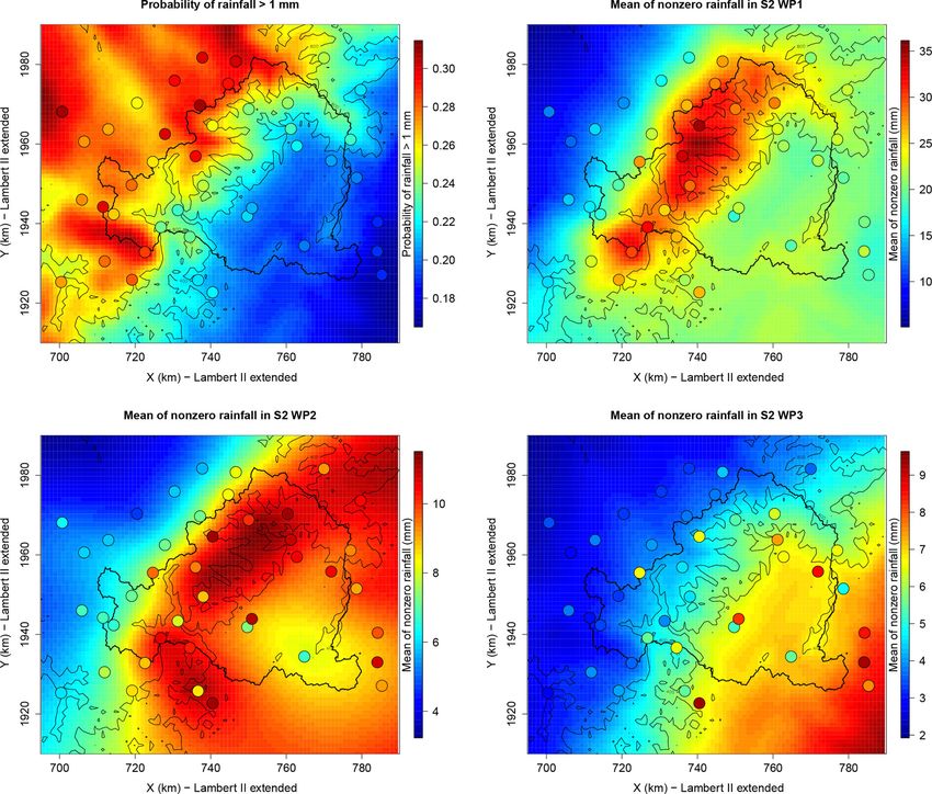
www.hydrol-earth-syst-sci.net/23/829/2019/ Hydrol. Earth Syst. Sci., 23, 829–849, 2019838 J. Blanchet et al.: Cross-validation framework for mapping rainfall hazard
Figure 4. (a) Monthly percentage of occurrence of the three WPs. (b) Boxplot of the monthly averages of daily nonzero rainfall. Each
boxplot contains 42 points (one point per station).
In cases where subsampling is also undertaken by season, NT , and two cross-validation scores – (12) and (21) –
we impose a restriction of S being two seasons, represent- of NRMSE, FF , NT and SPANT . For NT , we consider
ing the season-at-risk during which most of the annual max- T = 5 years, which is lower than the minimum length of
ima are observed, and the season-not-at-risk. Furthermore, the calibration data and allows one to focus on the tail
we impose the season-at-risk to be the same for all the sta- but still have several exceedances of the T -year return
tions due to the little extent of the region. Based on Fig. 4, we level at every station. So FF , by focusing on the maxi-
define the season-at-risk as the three months of September, mum of roughly 10 to 30 years of data, can be seen as
October and November, as in Garavaglia et al. (2010) and an evaluation score for the far tail, while N5 can be seen
Evin et al. (2016) for example. Alternative for bigger regions as an evaluation score for the close tail. For SPANT , we
would be to select the months composing the season-at-risk consider T = 100 and T = 1000 years in order to test
following the procedure described in Blanchet et al. (2015). extrapolation far in the tail but at a scale still commonly
used for engineering purposes (dam building, protec-
3.3.1 Marginal selection procedure tions, etc., Paquet et al., 2013).
The full cross-validation procedure for selecting both the 5. We repeat 50 times steps 1–4.
marginal and mapping models is summarized in Fig. 5. First We obtain 100 values of each calibration score and 100 val-
we consider the marginal distributions of Table 1 and select ues of each cross-validation score. We apply this procedure
the best of them at regional scale, as described in Sect. 3.1.2: to the four distributions of Table 1, considering the four al-
ternatives: no season nor WP (S = 1, K = 1), two seasons
1. We divide the days of 1948-2013 into two subsamples but no WP (S = 2, K = 1), no season but three WPs (S = 1,
of equal size, denoted C (1) and C (2) . Given the weak K = 3), two seasons and three WPs (S = 2, K = 3). Com-
temporal dependence of rainfall in the region (80 % of paring the distributions of the scores of the 16 models allows
the wet periods have length lower than 3), division is us the select the marginal distribution yielding to the best fit
made by randomly choosing blocks of five consecutive at regional scale. We select this marginal model for further
days to compose C (1) , the remaining blocks compos- consideration.
ing C (2) .
3.3.2 Mapping selection procedure
2. For every station i, we consider the set of observed days
(1) (2)
in C (1) and C (2) , giving Ci and Ci . Second we consider the mapping models of Sect. 3.2.1 for
interpolating the selected marginal model, and we select the
3. We fit each distribution of Table 1 to the two subsam-
(1) (2) best of them in two ways, as described in Sect. 3.2.2.
ples, getting estimates Ĝi and Ĝi of each distribu- (1,t)
tion and for every station. 1. We consider the estimates Ĝi , i = 1, . . . , Q, obtained
at the tth iteration of the marginal selection proce-
(1,t)
4. We compute the scores of Sect. 3.1.2, getting two cal- dure, and corresponding to the subsamples Ci , i =
ibration scores – (11) and (22) – of NRMSE, FF and 1, . . . , Q.
Hydrol. Earth Syst. Sci., 23, 829–849, 2019 www.hydrol-earth-syst-sci.net/23/829/2019/J. Blanchet et al.: Cross-validation framework for mapping rainfall hazard 839
4. We estimate the mapping models of Sect. 3.2.1, using
all the stations to make interpolation. We obtain new
estimates Ge∗(1,t) for each station i and each mapping
i
model.
5. We compute the spatial means of the TVD and KLD
e(1,t) , for,
e∗(1,t) to G
scores of Sect. 3.2.2, comparing G i i
i = 1, . . . , Q.
e(2,t) correspond-
6. We repeat steps 1–5 for the estimates G i
(2,t)
ing to the subsample Ci .
7. We repeat steps 1–6 for each of the 50 subsamples.
We obtain 200 values of each cross-validation score
NRMSE, FF , NT and SPAN, and 100 values of the TVD
and KLD scores. Comparing the distributions of these scores
allows us the select the mapping model yielding the smallest
score, for the selected marginal model. We select this map-
ping model for further consideration.
At this step we have selected the best marginal model and
the best mapping model (among those tested) for our data.
3.3.3 Final regional model
Finally, we consider the whole sample of data and apply the
selected marginal distribution and mapping model.
1. We estimate the selected marginal distribution Ĝ∗i based
on the full data, giving parameters θ̂ij∗ , i = 1, . . . , Q.
2. We estimate the mapping model associated with each
marginal parameter, using all θ̂ij∗ , i = 1, . . . , Q, to esti-
θj∗ (l).
mate the surface response e
We obtain estimates of pr(R(l) ≤ r|R(l) > 0) for every
l within the region, making full use of the observations. Es-
timation of pr(R(l) ≤ r) is obtained straightforwardly from
Eq. (3). Although not considered in this study, confidence in-
tervals could be obtained by bootstrapping within these two
last steps.
Figure 5. Schematic summary of the full cross-validation procedure
for selecting both the marginal and mapping models.
4 Results
2. We estimate the mapping models of Sect. 3.2.1 fol- 4.1 Selection of the marginal distribution
lowing the leave-one-out cross-validation framework of
Sect. 3.2.2. We obtain new estimates Ge(1,t) for each sta- We show in Fig. 6 the influence of considering seasons
i
tion i and each mapping model. Each G e(1,t) is a cross- and/or WPs in the marginal distributions, in the case of the
i
(1) (2)
validation estimation of both Gi and Gi since the Gamma distribution for illustration, but similar patterns are
e(1,t) did not use any data of station i. found with the other distributions. Figure 6 depicts the cross-
computation of G i validation scores of NRMSE, FF and N5 and the reliability
3. We compute the scores of Sect. 3.1.2 associated with score SPAN100 for the 100 split samples C (1) and C (2) . Cal-
e(1,t) , i = 1, . . . , Q. We obtain for each score two val-
G ibration scores are not shown because they are very similar
i
e(1,t) to the cross-validation scores (correlation 91 % between val-
ues (e.g., FF (11) and FF (21) when considering G i idation and calibration scores). For the stability criteria, we
and the maximum value over either C (1) or C (2) ). All
only show the values of SPAN100 , which corresponds to 3 to
these scores are cross-validation scores.
10 times the length of calibration data, but actually values
www.hydrol-earth-syst-sci.net/23/829/2019/ Hydrol. Earth Syst. Sci., 23, 829–849, 2019840 J. Blanchet et al.: Cross-validation framework for mapping rainfall hazard
Figure 6. Scores of cross-validation when Gs,k are Gamma distributions and the number of seasons and WP varies: S ∈ {1, 2} and K ∈ {1, 3}.
The values of (S, K) are indicated in the x labels. Each boxplot contains 100 points.
for T = 1000 years lead to the same conclusions (correlation Figure 7 illustrates this by showing the 95 % envelope of re-
99.9 % between SPAN100 and SPAN1000 ). turn level estimations over the 100 subsamples on either C (1)
Comparing the reliability scores NRMSE, FF and or C (2) together with the full sample of 35 years. Note that
N5 when neither season nor WP is used – case (1, 1) – with the envelopes do not show confidence intervals (that could
cases when either WPs – case (1, 3) – or seasons (case (2, be obtained by bootstrapping for example), but variability
1)) are considered shows there is at regional scale a clear im- when only half the data are used from calibration. Thus,
provement in using a mixture of Gamma distributions rather more than goodness-of-fit assessment, the plots of Fig. 7 al-
than considering a single Gamma for the whole year. Reli- low us to assess the quality of the fits at close extrapolation
ability criteria are slightly better (i.e., lower) when WPs are (i.e., when extrapolating at twice the length of the data). The
considered rather than season, but this is more marked for the plots clearly show that considering seasons and WPs allows
bulk of the distribution (represented by the NRMSE scores) us to get heavier-tailed distributions. The median estimates
than for its tail (FF and N5 ). Reliability scores are even bet- with two seasons and three WPs follow most closely the em-
ter when both seasons and WPs are considered – case (2, 3) pirical points, even the largest ones, showing the quality of
–, particularly for the tail of the distribution. the fits for extrapolating at twice the length of the data. How-
Obviously, there is a loss of stability when considering ever, we note that the return level plots of Fig. 7 all appear
seasons and/or WPs due to the increased number of param- approximately linear for high values, meaning that none of
eters. However, the score of SPAN100 ranges from 0.08 to the Gamma mixtures is able to produce heavy tails in the
0.14, which means that the two estimates of the 100-year re- sense of extreme value theory. It is possible that return levels
turn levels over C (1) and C (2) differ by 8 % to 14 %, which at extrapolation far beyond the observed return periods are
seems acceptable. underestimated. Figure 7 also shows that variability is rel-
We illustrate the quality of the fit for station Antraigues, atively low in all cases, although it naturally increases for
located in the very foothills of the Massif Central slope (see the marginal models involving more parameters. In particu-
Fig. 1), which shows among the largest annual maxima (see lar, the coefficient of variation of the 100-year return level
Fig. 2). We focus on the tail of the distribution by looking at with two seasons and three WPs is less than 7 %, in coher-
the return level plot (here beyond the yearly return period). ence with the SPAN100 of Fig. 6 at regional scale.
Of course, some variability is found in the return level es- Due to its better fit for the Gamma model (Figs. 6 and 7)
timations depending on the subsample used for estimation. as for the other distributions (not shown), we select the mix-
Hydrol. Earth Syst. Sci., 23, 829–849, 2019 www.hydrol-earth-syst-sci.net/23/829/2019/J. Blanchet et al.: Cross-validation framework for mapping rainfall hazard 841
Figure 7. Case of Antraigues when Gs,k are Gamma distributions and the number of seasons and WP varies: S ∈ {1, 2} and K ∈ {1, 3}. The
values of (S, K) are indicated in the title. The dotted lines show the 95 % envelope of return level estimates over the 100 subsamples. The
plain line shows the median estimates. The gray points show the full sample (35 years). Each estimation is based on half of these points.
Figure 8. Scores of cross-validation when Gs,k is either the extended exponential (eexp), extended generalized Pareto (egp),
Gamma (gamma), lognormal (lnorm) or Weibull (wei) distribution, with S = 2 and K = 3. Each boxplot contains 100 points. The boxplots
of reliability scores in the lognormal case are missing because they lie far above the upper range of depicted values.
ture model with S = 2 seasons and K = 3 WPs for further alized Pareto, itself closely followed by the Weibull model.
investigation. Figure 8 shows the scores of cross-validation A closer look at the values of ffi and ni,5 for all stations
when the parent distribution Gs,k is either the extended expo- and samples reveals that the weaker reliability of the Weibull
nential, extended generalized Pareto, Gamma, lognormal or and extended generalized Pareto models is due to their ten-
Weibull distribution. The reliability scores NRMSE, FF and dency to systematically overestimate the probability of oc-
N5 in the lognormal case are missing because they lie far currence of large values (i.e., to underestimate their return
above the upper range of the depicted values (e.g., the me- period), with ffi and ni,5 tending to be too frequently small
dian NRMSE is about 0.7), which clearly rules out the use of (see case G1 of Fig. 3). Note that the lack of reliability of the
the lognormal model for this region. The reliability criteria of extended generalized Pareto in the upper tail is at least par-
the four other distributions all show the same pattern: a better tially attributable to being based on fitting the entire range of
performance of the Gamma model, closely followed by the rainfall values, which leads to a systematic overestimation of
extended exponential case. Then comes the extended gener- the shape parameter ξ in Table 1 compared to when fitting a
www.hydrol-earth-syst-sci.net/23/829/2019/ Hydrol. Earth Syst. Sci., 23, 829–849, 2019You can also read