The 21st-century fate of the Mocho-Choshuenco ice cap in southern Chile - The Cryosphere
←
→
Page content transcription
If your browser does not render page correctly, please read the page content below
The Cryosphere, 15, 3637–3654, 2021
https://doi.org/10.5194/tc-15-3637-2021
© Author(s) 2021. This work is distributed under
the Creative Commons Attribution 4.0 License.

The 21st-century fate of the Mocho-Choshuenco ice cap
in southern Chile
Matthias Scheiter1,a , Marius Schaefer2 , Eduardo Flández3 , Deniz Bozkurt4,5 , and Ralf Greve6,7
1 Research   School of Earth Sciences, Australian National University, Canberra, Australia
2 Instituto de Ciencias Físicas y Matemáticas, Universidad Austral de Chile, Valdivia, Chile
3 Departamento de Física, Facultad de Ciencias, Universidad de Chile, Santiago, Chile
4 Departamento de Meteorología, Universidad de Valparaíso, Valparaíso, Chile
5 Center for Climate and Resilience Research (CR)2, Santiago, Chile
6 Institute of Low Temperature Science, Hokkaido University, Sapporo, Japan
7 Arctic Research Center, Hokkaido University, Sapporo, Japan
a formerly at: Institut für Geophysik und Geoinformatik, TU Bergakademie Freiberg, Freiberg, Germany

Correspondence: Matthias Scheiter (matthias.scheiter@anu.edu.au)

Received: 8 October 2020 – Discussion started: 11 November 2020
Revised: 23 June 2021 – Accepted: 25 June 2021 – Published: 6 August 2021

Abstract. Glaciers and ice caps are thinning and retreat-        different global climate models and on the uncertainty asso-
ing along the entire Andes ridge, and drivers of this mass       ciated with the variation of the equilibrium line altitude with
loss vary between the different climate zones. The south-        temperature change. Considering our results, we project a
ern part of the Andes (Wet Andes) has the highest abun-          considerable deglaciation of the Chilean Lake District by the
dance of glaciers in number and size, and a proper under-        end of the 21st century.
standing of ice dynamics is important to assess their evo-
lution. In this contribution, we apply the ice-sheet model
SICOPOLIS (SImulation COde for POLythermal Ice Sheets)
to the Mocho-Choshuenco ice cap in the Chilean Lake Dis-         1   Introduction
trict (40◦ S, 72◦ W; Wet Andes) to reproduce its current state
and to project its evolution until the end of the 21st cen-      Most glaciers and ice caps in the Andes are currently thin-
tury under different global warming scenarios. First, we cre-    ning and retreating (e.g. Braun et al., 2019), and rates of mass
ate a model spin-up using observed surface mass balance          loss are increasing in many places (Dussaillant et al., 2019).
data on the south-eastern catchment, extrapolating them to       In the southernmost part of the Andes (36–56◦ S), which is
the whole ice cap using an aspect-dependent parameteriza-        called the Wet Andes or Patagonian Andes in the literature
tion. This spin-up is able to reproduce the most important       (Lliboutry, 1998), the highest number of glaciers are found,
present-day glacier features. Based on the spin-up, we then      and large ice fields such as the Northern Patagonia Ice Field,
run the model 80 years into the future, forced by projected      Southern Patagonia Ice Field, and Cordillera Darwin are lo-
surface temperature anomalies from different global climate      cated in this region. The specific mass losses observed or in-
models under different radiative pathway scenarios to obtain     ferred for the glaciers of the Wet Andes are the highest in
estimates of the ice cap’s state by the end of the 21st cen-     the Andes (Dussaillant et al., 2019; Braun et al., 2019) and
tury. The mean projected ice volume losses are 56 ± 16 %         among the highest of all glacier regions worldwide (Zemp
(RCP2.6), 81 ± 6 % (RCP4.5), and 97 ± 2 % (RCP8.5) with          et al., 2019).
respect to the ice volume estimated by radio-echo sounding          The maritime climate of the Wet Andes is characterized
data from 2013. We estimate the uncertainty of our projec-       by high precipitation rates of up to 10 m yr−1 on the wind-
tions based on the spread of the results when forcing with       ward side and rather mild temperatures with freezing levels
                                                                 generally above 1 km above mean sea level with an over-

Published by Copernicus Publications on behalf of the European Geosciences Union.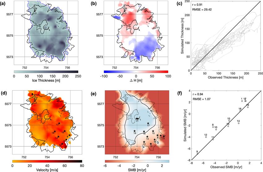
3638                          M. Scheiter et al.: The 21st-century fate of the Mocho-Choshuenco ice cap in southern Chile

all modest seasonality (Garreaud et al., 2013). This leads          Table 1. Comparison between simulated and observed velocities at
to an exceptionally high mass turnover (Schaefer et al.,            stakes where velocity observations are available from Geoestudios
2013, 2015, 2017) and high flow speeds for the glaciers in the      (2013).
region (Sakakibara and Sugiyama, 2014; Mouginot and Rig-
not, 2015). In addition to climate forcings, other important            Stake            B8      B10    B12    B14    B15    B17    B18
contributors to glacier change in the region are ice dynamics           vobs(m yr−1 )    22.2    12.7   60.3   33.8   19.4   31.2   27.2
and frontal ablation. Ice-flow models incorporate these pro-            vsim (m yr−1 )   11.6    13.7   35.9   20.2   20.7   18.6   20.5
cesses and are therefore appropriate tools to project the future
behaviour of the glaciers of the Wet Andes.
   Only a few studies have tried to project future be-              We conclude the paper by summarizing the main findings in
haviour of Andean glaciers. Réveillet et al. (2015) mod-            Sect. 5.
elled Zongo Glacier (16◦ S) in the tropical Andes using the
three-dimensional full-Stokes model Elmer/Ice (developed
by Gagliardini et al., 2013). They projected volume losses          2     Methods
between 40 % and 89 % by the end of this century under
the RCP2.6 and RCP8.5 scenarios, respectively. In the Wet           2.1     Observational data
Andes, Möller and Schneider (2010) projected an area loss
                                                                    The ice cap on which we focus in this study covers the
of 35 % of Glaciar Noroeste, an outlet glacier of the Gran
                                                                    Mocho-Choshuenco volcanic complex, which is located at
Campo Nevado ice cap (53◦ S), by the end of the 21st century
                                                                    40◦ S, 72◦ W (see inset map in Fig. 1). Over the last
using a degree-day model and volume-area scaling relation-
                                                                    20 years, climatological and glaciological observations have
ships. Schaefer et al. (2013) modelled the surface mass bal-
                                                                    been made on the ice cap (Rivera et al., 2005; Schaefer
ance (SMB) of the Northern Patagonian Ice Field in the 21st
                                                                    et al., 2017). SMB data were obtained through the traditional
century under the A1B scenario (of Assessment Report 4
                                                                    glaciological method on a stake network on the south-eastern
from the Intergovernmental Panel on Climate Change, IPCC;
                                                                    part of the ice cap (red stars in Fig. 1). These measurements
comparable to RCP6.0). They projected a strongly decreas-
                                                                    reported by Schaefer et al. (2017) yielded an average neg-
ing SMB until the end of the 21st century mainly due to an
                                                                    ative SMB of −0.9 m w.e. yr−1 (metre water equivalent per
increase in surface temperature by the middle of the century
                                                                    year) with a high mass turnover of around 2.6 m w.e. yr−1
and a decrease in accumulation towards the end of the cen-
                                                                    (see Sect. 2.4). This high mass turnover is a consequence
tury. Collao-Barrios et al. (2018) infer important committed
                                                                    of the interaction between high precipitation rates leading
mass loss of San Rafael Glacier under current climate apply-
                                                                    to high accumulation rates and high temperatures leading to
ing the Elmer/Ice flow model with fixed glacier outlines.
                                                                    high melt rates. In this respect, climatological data (2006 to
   In this contribution, our first objective is to reproduce the
                                                                    2015) indicate that the annual mean temperature was 2.6 ◦ C
present-day behaviour of the Mocho-Choshuenco ice cap in
                                                                    at an automatic weather station (green circle in Fig. 1) at an
the northern part of the Wet Andes (40◦ S) using the ice-
                                                                    elevation of 2000 m and therefore close to the typical equilib-
sheet model SICOPOLIS (SImulation COde for POLyther-
                                                                    rium line altitude (ELA) (Schaefer et al., 2017). Mean annual
mal Ice Sheets) (Greve, 1997a, b). To this end, we make
                                                                    precipitation over the same period was around 4000 mm yr−1
use of a newly developed SMB parameterization scheme and
                                                                    in Puerto Fuy at an elevation of 600 m to the north of the vol-
glaciological data obtained on the ice cap to calibrate the
                                                                    cano, and orographic precipitation effects lead to a relatively
model and reproduce its current state. Our second objective
                                                                    high amount of precipitation on the ice cap.
is to project the behaviour of the Mocho-Choshuenco ice cap
                                                                       At some of the mass balance stakes (red stars with inner
through the course of the 21st century to provide one of the
                                                                    black dots in Fig. 1), high precision GPS measurements were
first constraints on future glacier dynamics in the Wet Andes.
                                                                    made in July and October 2013 to infer surface flow velocity
For this aim, we make use of temperature projections from
                                                                    (Geoestudios, 2013), and the observed velocities are shown
23 global climate models (GCMs) participating in the Cou-
                                                                    in Table 1. Further measurements include ground penetrating
pled Model Intercomparison Project phase 5 (CMIP5) (Tay-
                                                                    radar (GPR) transects (green lines in Fig. 2a) over most parts
lor et al., 2012) under low (RCP2.6), medium (RCP4.5), and
                                                                    of the ice cap (Geoestudios, 2014). Through inverse distance
high (RCP8.5) emission scenarios as input to SICOPOLIS.
                                                                    weighting interpolation over the whole ice cap, a total ice
   We begin this paper by describing the observational data
                                                                    volume of 1.038 km3 was obtained (Geoestudios, 2014). The
and methods (Sect. 2). In Sect. 3, we present the results. First,
                                                                    interpolated ice thickness map was subtracted from a dig-
we validate the model spin-up using observed SMB, glacier
                                                                    ital elevation model (TanDEM WorldDEM™, acquired be-
outlines, ice thickness, and flow speed. We then present the
                                                                    tween 2012 and 2014) to yield a bedrock topography (Flán-
evolution of ice cap extension and volume during the 21st
                                                                    dez, 2017). We use this topography as the base of the ice cap
century as obtained through different emission scenarios.
                                                                    in the simulations we perform with SICOPOLIS.
Then, in Sect. 4, we discuss our results, compare them to
previous studies, and analyse the limitations of our approach.

The Cryosphere, 15, 3637–3654, 2021                                                           https://doi.org/10.5194/tc-15-3637-2021
M. Scheiter et al.: The 21st-century fate of the Mocho-Choshuenco ice cap in southern Chile                                  3639

Figure 1. Overview map of the Mocho-Choshuenco ice cap with significant geographic features and measurement sites. The contour line
spacing is 50 m. East and north are in UTM S18. Background: Landsat image (22 February 2015). Inset map shows location in South
America.

2.2   SICOPOLIS                                                     served cyclic surge behaviour under constant, present-day
                                                                    climate conditions. For this study, we adapted SICOPOLIS
                                                                    v5-dev (Greve and SICOPOLIS Developer Team, 2021) for
The three-dimensional, dynamic and thermodynamic model              the Mocho-Choshuenco ice cap in SIA mode. The horizontal
SICOPOLIS was originally created in a version for the               resolution is 100 m. In the vertical, we use terrain-following
Greenland ice sheet (Greve, 1997a, b). Since then, the model        coordinates (sigma transformation) with 81 layers. The time
has been developed continuously and applied to problems             step for the numerical integration is 0.01 years. We employ a
of past, present, and future glaciation of Greenland, Antarc-       standard Glen flow law with a stress exponent of n = 3. Basal
tica, the entire Northern Hemisphere, the polar ice caps of         sliding is modelled by a linear sliding law,
the planet Mars, and other places, resulting in more than
120 publications in the peer-reviewed literature (http://www.       vb = −Cb τb ,                                              (1)
sicopolis.net, last access: 3 August 2021). The model sup-
ports the shallow-ice approximation (SIA) for slow-flowing          where vb is the basal sliding velocity, τb the basal drag, and
grounded ice, hybrid shallow-ice–shelfy stream dynamics for         Cb the sliding coefficient. The value of the latter is deter-
fast-flowing grounded ice, and the shallow-shelf approxima-         mined by the calibration procedure of the present-day spin-
tion for floating ice (Bernales et al., 2017), as well as several   up (see Sect. 3.1). Since Mocho-Choshuenco is a temperate
thermodynamics solvers (Blatter and Greve, 2015; Greve and          ice cap, we do not solve the energy balance equation. Rather,
Blatter, 2016).                                                     we keep the temperature at a constant value of 0 ◦ C (precisely
   Mainly developed for ice sheets, the smallest ice body to        speaking, and for technical reasons only as SICOPOLIS does
which SICOPOLIS has been applied so far is the Austfonna            not allow an all-temperate ice body, −0.001 ◦ C). The rate
Ice Cap, for which Dunse et al. (2011) reproduced the ob-           factor is set to the value recommended by Cuffey and Pa-

https://doi.org/10.5194/tc-15-3637-2021                                                  The Cryosphere, 15, 3637–3654, 2021
3640                           M. Scheiter et al.: The 21st-century fate of the Mocho-Choshuenco ice cap in southern Chile

Figure 2. (a) Ground penetrating radar (GPR) transects shown in green lines together with the interpolated ice thickness. (b) Bedrock
topography obtained after subtracting the interpolated ice thickness from surface elevation. This topography is used as the ice cap base in our
simulations.

terson (2010) for 0 ◦ C, which is A = 2.4 × 10⁻²⁴ s−1 Pa−3 .              imum BELA − AELA in the opposite direction, and a mean
To ensure proper mass conservation despite the steep slopes               value BELA in the two perpendicular directions.
and rugged bed topography, we use an explicit solver for the                These values can be summarized in a cosine function in ϕ
ice thickness equation that discretizes the advection term by             with the direction of maximum ELA ϕ0 , the amplitude AELA ,
a mass-conserving scheme in an upwind flux form (Calov                    and an offset of the average ELA BELA :
et al., 2018).
                                                                          ELA = AELA cos(ϕ − ϕ0 ) + BELA .                                 (3)
2.3    Aspect-dependent SMB parameterization                              BELA is used to shift the ELA to the desired mean altitude, ϕ
                                                                          is the cardinal direction of a point with respect to the summit,
SICOPOLIS incorporates a linear altitude-dependent SMB                    and it can be calculated by
parameterization which is visualized in Fig. 3a and can be
described by the following formula:                                       ϕ = arctan2(x − xsum , y − ysum ),                               (4)
                                                                          where arctan2 denotes the two-argument arctangent, and x
SMB(C) = min(S0 , M0 · (z(C) − ELA)).                            (2)      and y are the distances in the two directions from a grid point
                                                                          to the summit location (xsum , ysum ).
Here, ELA is the equilibrium line altitude, z(C) is the evolv-
ing ice surface elevation of a specific grid cell C, M0 denotes           2.4   Transient spin-up
the mass balance gradient, and S0 is maximum SMB.
   From the simulations performed by Flández (2017) on the                Before being able to make future projections for the Mocho-
Mocho-Choshuenco ice cap, it becomes apparent that the                    Choshuenco ice cap, we first aim to reproduce its current
simple altitude-dependent SMB parameterization in Eq. (2)                 state. Due to the observed negative SMB at present, we aim
is not detailed enough to account for small-scale SMB vari-               to build a transient spin-up that represents a shrinking ice
ations in the ice cap. In particular, SMB should be lower in              cap. This is achieved in two steps: first, we build a theoretical
the north-western part than in the south-eastern part of the              steady state of the ice cap in the late 1970s and then run the
ice cap due to the aspect dependence of solar radiation and               model from 1979 to 2013 with ERA5 near-surface air tem-
snow redistribution (wind drift) which during precipitation               perature data (see Fig. 4). This 35-year period is justified by
events predominantly blows from the north-west. We there-                 the turnover time τ , which is a typical timescale for a glacier
fore employ a new parameterization which is illustrated in                defined by
Fig. 3b. With Mocho’s summit in the centre, ELA should                           [H ]
have a maximum BELA + AELA in the direction ϕ0 , a min-                   τ=          ,                                                    (5)
                                                                                [SMB]

The Cryosphere, 15, 3637–3654, 2021                                                            https://doi.org/10.5194/tc-15-3637-2021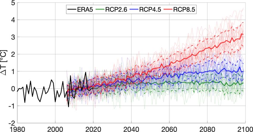
M. Scheiter et al.: The 21st-century fate of the Mocho-Choshuenco ice cap in southern Chile                                                   3641

Figure 3. (a) Elevation-dependent SMB parameterization. SMB increases linearly with elevation until an upper bound S0 and stays constant
at higher elevations. (b) Aspect-dependent SMB parameterization. Equilibrium line altitude (ELA) takes a minimum and maximum on two
opposite directions (BELA ±AELA ) and their mean (BELA ) on perpendicular directions. ϕ0 is a direction offset to rotate the values according
to the atmospheric conditions. In this visualization, ϕ0 is set to 315◦ , the value used in this study, and (xsum , ysum ) indicates the position of
Mocho’s summit.

where [H ] is the typical ice thickness and [SMB] the typ-                  by 18 m in 1979 with respect to the state in 2013, accord-
ical SMB (e.g. Greve and Blatter, 2009). By taking [H ] =                   ing to the ELA-temperature gradient of 88 m K−1 which we
Vobs /Aobs (where Vobs = 1.038 km3 is the observed ice vol-                 determine in Sect. 2.6. Afterwards, we adjust the model pa-
ume and Aobs = 15.1 km3 the observed area) and [SMB] =                      rameters mean ELA (BELA ), ELA amplitude (AELA ), maxi-
2.6 m w.e. yr−1 (computed as the mean of the absolute val-                  mum SMB (S0 ), SMB gradient (M0 ), direction of maximum
ues from the observed SMB at the stakes), we obtain τ ≈                     ELA (ϕ0 ), and sliding coefficient (Cb ) in order to match the
27 years. This is slightly less than the 35-year period of                  present-day observations of SMB, ice thickness, ice extent,
ERA5 data, which therefore should be sufficient to produce                  ice volume, and surface velocity of the ice cap. While the pa-
a valuable spin-up for the year 2013.                                       rameters defining the SMB parameterization were calibrated
   ERA5 is a state-of-the-art global reanalysis produced by                 under observational constraints, Cb was purely used as a cali-
the European Centre for Medium-Range Weather Forecasts                      bration parameter. We discuss this in more detail in Sect. 4.1.
(ECMWF). It combines large amounts of historical obser-                     It is important to note that the steady-state spin-up in the
vations into global estimates using advanced modelling sys-                 1970s is a theoretical construct as the glacier had been losing
tems and data assimilation, i.e. Integrated Forecasting Sys-                mass before this period and was not in a steady state. It is
tem (Cycle 41r2) (Hersbach et al., 2020). ERA5 has a spatial                only to be interpreted as a first step in order to get an accu-
resolution of 0.25◦ × 0.25◦ (∼ 30 km) and vertical resolution               rate representation of the shrinking ice cap in 2013 with its
of 137 levels from the surface to a height of 80 km.                        negative SMB.
   Given that there are no available long-term surface me-
teorological data around the ice cap, we contrasted 700 hPa                 2.5    Temperature projections
ERA5 temperature data against the radiosonde data (Inte-
grated Global Radiosonde Archive v2, available at https:
                                                                            The main goal of this study is to project the future evolu-
//www1.ncdc.noaa.gov/pub/data/igra/, last access: 11 Febru-
                                                                            tion of the Mocho-Choshuenco ice cap. We use future tem-
ary 2021) from Puerto Montt (41.5◦ S, 72.9◦ W) for the
                                                                            perature simulations from 23 climate models participating in
period 1979–2019. This is due to the fact that Schaefer
                                                                            CMIP5 (see Appendix A). To ease the calculations, all the
et al. (2017) found a very good correlation between the
                                                                            models were interpolated onto a common grid of 1.5◦ × 1.5◦
700 hPa pressure level temperature from the radiosonde data
                                                                            using bilinear interpolation. Then the time series of each
at Puerto Montt and temperature measured at the Mocho au-
                                                                            model were extracted from the grid point corresponding to
tomatic weather station. In this respect, ERA5 shows rea-
                                                                            Mocho-Choshuenco ice cap (40◦ S, 72◦ W). As the model
sonable skills in capturing the long-term regional tempera-
                                                                            trajectories start in 2006 and in order to be consistent with
ture trend (+0.19 ◦ C in 41 years) detected in the radiosonde
                                                                            the reference ice cap conditions based on the observational
data (+0.22 ◦ C in 41 years) with a high temporal correlation
                                                                            dataset obtained between 2009 and 2013, we used the pe-
(0.77).
                                                                            riod from 2006 to 2020 as the reference period rather than
   Due to this temperature increase of around 0.2 ◦ C, we
                                                                            the commonly used historical periods (e.g. 1976–2005) in
build the steady state by lowering the mean ELA (BELA )
                                                                            order to construct projections of temperature anomalies. For

https://doi.org/10.5194/tc-15-3637-2021                                                              The Cryosphere, 15, 3637–3654, 2021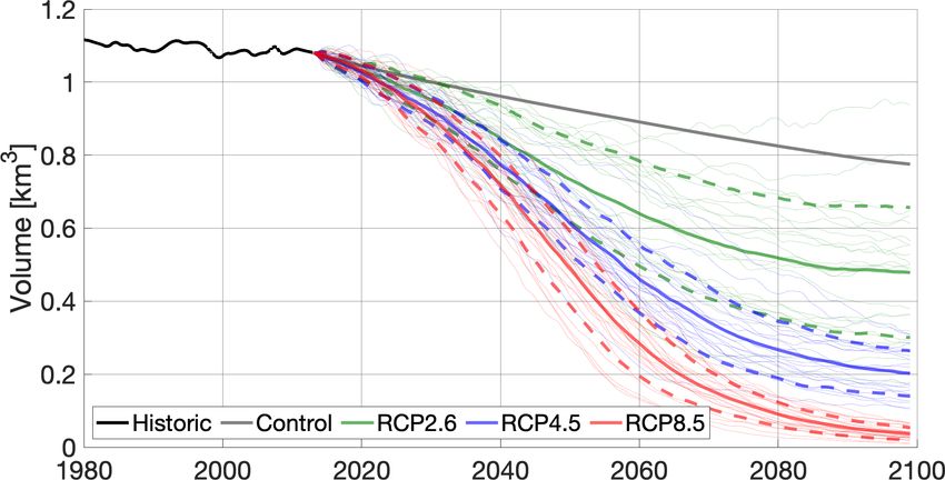
3642 M. Scheiter et al.: The 21st-century fate of the Mocho-Choshuenco ice cap in southern Chile
Figure 4. Temperature projections for the Mocho-Choshuenco ice cap through the 21st century for three different scenarios, RCP2.6, RCP4.5,
and RCP8.5, along with historical ERA5 data which are used for the transient spin-up. The thin lines show projections of the 23 individual
climate models, thick solid lines indicate their mean, and thick dashed lines indicate the 1σ confidence interval. The period between 2006
and 2020 is used as the reference period for each individual model.
each of the individual models, the mean temperature between lutions after the 2050s with weaker projected changes than
2006 and 2020 was then subtracted from the whole time those in RCP8.5. By the end of the century, projected tem-
series, leading to anomaly temperature projections with re- perature increases for the RCP2.6 and RCP4.5 scenarios are
spect to this period. At the final step, the SICOPOLIS model 0.33 ± 0.47 and 1.01 ± 0.43 ◦ C, respectively.
was driven by each of the 23 model projections to provide a
more robust assessment of the future evolution of the Mocho- 2.6 Glacier sensitivity to temperature change
Choshuenco ice cap. This allows us to assess the uncertainty
associated with climate model differences. In addition to the To link the projected 21st-century temperature rise to ice
future projections, we also include a control run in our anal- dynamics, it is necessary to relate the temperature anoma-
ysis in which we run the model for the period 2013–2100 lies to changes in SMB, which is determined by the mean
with zero temperature anomaly with respect to the reference ELA (BELA ) in our case. We assume that temperature is the
period 2006–2020. This enables us to calculate a committed only influencing factor on the projected net SMB without ex-
mass loss and assess the influence of ice dynamics alone, in- plicitly distinguishing between precipitation and runoff. Fur-
dependent of future temperature increase. ther, we focus on annual rather than melt-season tempera-
Our approach makes use of three emission scenarios fol- ture projections as the climate models project both to be very
lowing the IPCC protocols (IPCC, 2013): high-mitigation, close to each other in the Mocho-Choshuenco volcanic com-
Paris Agreement compatible (RCP2.6); medium stabilization plex. There are 4 years (2009–2013) when both the ELA and
scenario with a peak around 2040, then decline (RCP4.5); annual mean temperature at a similar altitude are available
and high-end baseline scenario with no control policies of (Schaefer et al., 2017). These data are shown in Fig. 5, to-
greenhouse gas emissions (RCP8.5). This allows us to con- gether with the ELA error estimates.
trast the future evolution of the Mocho-Choshuenco ice cap In order to predict the ELA for any temperature, we
under different emission scenarios, together with the uncer- first assume a linear relationship between both and solve a
tainty introduced by future emissions. Figure 4 shows the weighted least squares problem to find the slope and inter-
projected changes in temperature obtained from 23 individ- cept (i.e. ELA gradient and ELA for 0 ◦ C). ELA predictions
ual climate models for the ice cap under the three different for any temperature {Ti , Tj , . . .} can be made by multiplying
emission scenarios until the end of the century. This yields the forward operator Ĝ with the vector m containing both
69 projections which are all used to run SICOPOLIS and are model parameters:
averaged afterwards. All projections follow a similar trend
until the 2040s, when the RCP8.5 scenario separates from the
ELA = Ĝm = ĜN (µ, 6) = N Ĝµ, Ĝ6 ĜT ,
others and continues to increase throughout the century, lead-
ing to a model mean temperature increase of 3.15 ± 0.69 ◦ C
Ti 1
by the end of the century. The temperature projections under
Ĝ = Tj 1 , (6)
the RCP2.6 and RCP4.5 scenarios have largely similar evo- .. ..
. .
The Cryosphere, 15, 3637–3654, 2021 https://doi.org/10.5194/tc-15-3637-2021M. Scheiter et al.: The 21st-century fate of the Mocho-Choshuenco ice cap in southern Chile 3643
Since the temperature projections give anomalies with re-
spect to the period 2006–2020, we only rely on relative rather
than absolute temperatures. Therefore, we convert the tem-
perature changes into changes of ELA with the parameter
µ1 = 88 m K−1 , which means that the ELA increases by 88 m
per ◦ C temperature increase. We assess the uncertainty prop-
agation of this parameterization through the ice flow simu-
lation code by performing additional
√ experiments with up-
per and lower ELA gradients µ1 ± 611 = (88±37) m K−1 ,
which corresponds to the 1σ confidence interval.
Figure 5. Relationship between annual temperature and ELA on 3 Results
Mocho-Choshuenco ice cap. The error bars indicate the error as es-
timated by Schaefer et al. (2017). The relationship between ELA 3.1 Spin-up and model calibration
and temperature was found through weighted linear regression.
Following the spin-up and calibration procedure explained in
where m is distributed according to a bivariate normal distri- Sect. 2.4, we tune the model to find the following optimal pa-
bution N (µ, 6) with mean vector µ and model covariance rameters: BELA = 2050 m, AELA = 87.5 m, S0 = 2.2 m yr−1
matrix 6 (e.g. Aster et al., 2018): and Cb = 1.0 × 10⁻⁴ m yr−1 Pa−1 , M0 = 0.027 yr−1 , and
ϕ0 = 315◦ . We discuss the physical plausibility of these val-
m ∼ N (µ, 6) , ues in Sect. 4.1.
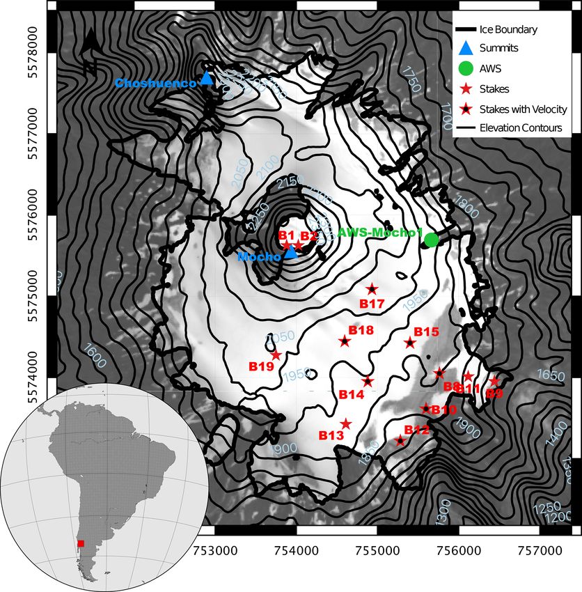
−1 The spin-up is evaluated against observations in Fig. 6.
µ = ĜT 6 −1
d Ĝ ĜT 6 −1
d d̂, Figure 6a shows the thickness distribution and extent of the
−1 simulated ice cap. The model captures the general outlines
6 = ĜT 6 −1
d Ĝ . (7) of the ice cap with only small inaccuracies at some outlet
tongues. In Fig. 6b, we compare the simulated and observed
Inserting the observed data, we identify the forward operator ice thickness. Overall, the simulations overestimate ice thick-
Ĝ, the data covariance matrix 6 d , and the vector of observed ness in the northern part of the ice cap and underestimate
ELAs d̂ as it in the south-east. Figure 6c shows that the simulated ice
T1 1
2
σ1 0 0 0
thickness is in reasonable agreement with observations along
T2 1 2 the radar profiles, with a high correlation (0.91), and the root
, 6 d = 0 σ2 0 0
Ĝ = , mean square error (RMSE) that is around 13 % of the maxi-
T3 1 0 0 σ32 0
T4 1 0 0 0 σ42 mum measured ice thickness.
The velocity map in Fig. 6d shows velocities of less than
ELA1 50 m yr−1 on most parts of the ice cap, matching well with
ELA2
d̂ = (8) the observed low velocities that were measured in spring
ELA3 .
2013 (Geoestudios, 2013). Stakes where velocity measure-
ELA4 ments are available are marked with black stars in Fig. 6d.
Predictions for a general temperature T can be made through Observed and modelled velocities at these locations are com-
pared in Table 1, showing an overall good agreement (RMSE
of 12.5 m yr−1 ), with simulated velocities being on average
ELA(T ) = N µ1 T + µ2 , 611 T 2 + 2612 T + 622 , (9)
9.4 m yr−1 lower. However, the modelled velocities represent
with a yearly average, whereas the velocity measurements were
taken in the spring season, making a direct comparison diffi-
88 m K−1
µ= , cult, and these values should only be seen as a rough orien-
1777 m tation.
1365 m2 K−2 −2203 m2 K−1 The simulated SMB in Fig. 6e matches well with ob-
6= , (10) servations reported by Schaefer et al. (2017) with the ob-
−2203 m2 K−1 3657 m2
served SMB distribution, SMB gradient, and ELA on the
where µ1 = 88 m K−1 is our estimated increase in ELA per south-eastern catchment. Figure 6f shows a direct compar-
degree Celsius, and µ2 = 1777 m is the ELA that we would ison of modelled SMB at the stake locations and the respec-
obtain for a yearly average temperature of 0 ◦ C. Figure 5 tive observations. The fit is very good, with a high correlation
shows the mean of ELA predictions against temperature, to- (0.94), and the RMSE corresponds to roughly 11 % of the ab-
gether with the 1σ confidence interval. solute range between highest and lowest observed SMB.
https://doi.org/10.5194/tc-15-3637-2021 The Cryosphere, 15, 3637–3654, 20213644 M. Scheiter et al.: The 21st-century fate of the Mocho-Choshuenco ice cap in southern Chile
Figure 6. Results of the transient spin-up for 2013. (a) Ice thickness distribution with observed (black) and modelled (blue) extent, (b) dif-
ference between modelled and observed ice thickness, (c) modelled thickness against observed thickness along radar profiles, (d) surface
flow velocity and stakes with velocity observations, (e) modelled surface mass balance over model domain with SMB stakes as black stars
and simulated ELA as solid black line, and (f) modelled SMB against observed SMB at stakes.
3.2 Projected future evolution of the ice cap ments between the ensemble members. For the RCP4.5 sce-
nario, this is only the case until the 2060s, and as the mean
The evolution of the total ice volume under the RCP2.6, curve flattens, the uncertainties remain constant. The uncer-
RCP4.5, and RCP8.5 scenarios, as well as the control run tainty of the RCP8.5 scenario increases until the 2050s and
with a zero-anomaly with respect to the reference period then decreases until the year 2100. These contrasts in the pro-
2006–2020, is shown in Fig. 7. For the control run, the ice jections under different emission scenarios reflect the higher
cap loses 28 % of its volume by 2100, which can be inter- signal-to-noise ratio for the RCP8.5 scenario as this scenario
preted as the committed loss due to the non-steady-state con- has a more prominent temperature increase (also see Fig. 4).
ditions during the reference period. The projections for the Projected ice volumes and uncertainties for different scenar-
23 individual climate models (thin lines) can be summarized ios and years are summarized in Table 2.
by the multimodel ensemble mean (thick solid lines) and 1σ In addition to the uncertainty introduced by different cli-
confidence interval (thick dashed lines). All three scenarios mate models, we analyse the impact that the ELA depen-
start with a negative slope and lose mass at a similar rate, re- dence on temperature has on glacier projections. We average
flecting the present-day negative SMB. From the 2050s, the the 23 climate model temperature projections for the three
scenarios begin to diverge significantly, indicating that the scenarios before running SICOPOLIS instead of forcing it
differences between temperature increases of each projection individually with each climate model as in the previous sec-
start to dominate the ice dynamics. By the end of the century, tions. With these mean projections, we perform three model
all mean curves flatten out. runs for each scenario: the mean gradient between temper-
In terms of variability between the climate models, the ature and ELA (88 m K−1 ) and the upper and lower bound
RCP2.6 scenario starts with a narrow confidence interval of the 1σ confidence interval (51 and 125 m K−1 ). The re-
which gets larger throughout the century, reflecting disagree- sulting ice volume evolutions are shown in Fig. 8. The mean
The Cryosphere, 15, 3637–3654, 2021 https://doi.org/10.5194/tc-15-3637-2021M. Scheiter et al.: The 21st-century fate of the Mocho-Choshuenco ice cap in southern Chile 3645
Figure 7. Ice volume evolution under the three scenarios RCP2.6 (green), RCP4.5 (blue), and RCP8.5 (red) until the year 2100. Thin lines
show the 23 individual evolutions from different climate models, thick solid lines indicate their mean, and thick dashed lines indicate the
mean plus and minus the standard deviation. The solid black line shows the evolution of the transient spin-up between 1979 and 2013, and
the thick grey line shows a control run based on a zero-anomaly with respect to the reference period 2006–2020.
Table 2. Projected ice volumes in cubic metres for different sce- Table 3. Projected maximum ice thickness in metres for different
narios and years: mean and standard deviation obtained by forcing scenarios and years: mean and standard deviation obtained by forc-
SICOPOLIS for 23 climate models. ing SICOPOLIS for 23 climate models.
Year RCP2.6 RCP4.5 RCP8.5 Year RCP2.6 RCP4.5 RCP8.5
2013 1.08 1.08 1.08 2013 225.5 225.5 225.5
2040 0.85 ± 0.09 0.77 ± 0.07 0.72 ± 0.08 2040 191.1 ± 23.7 187.1 ± 14.7 186.9 ± 11.1
2060 0.64 ± 0.14 0.46 ± 0.09 0.28 ± 0.09 2060 186.9 ± 45.6 184.7 ± 45.0 176.9 ± 24.4
2080 0.52 ± 0.17 0.27 ± 0.08 0.09 ± 0.03 2080 186.8 ± 78.1 181.2 ± 44.0 145.2 ± 24.8
2099 0.48 ± 0.18 0.2 ± 0.06 0.04 ± 0.02 2099 186.8 ± 86.9 178.4 ± 60.5 91.0 ± 42.4
curves are very similar to those obtained in Fig. 7; however, before 2080, and afterwards the reduction in ice thickness is
the spread is higher for the RCP4.5 and RCP8.5 scenarios less pronounced.
and lower for the RCP2.6 scenario with respect to those ob- The high-end scenario (RCP8.5) shows a clearly differ-
tained in Fig. 7. ent pattern in both thinning and retreat over the 21st century.
The ice volume loss can be broken down into thinning and While the thickness pattern for 2040 is comparable to the two
retreat, i.e. to a lower ice thickness and a smaller ice area, other scenarios, ice loss clearly accelerates between 2040 and
respectively, towards the end of the century. Figure 9 shows 2080. This can be discerned by the faint colours in the last
the evolution of the ice thickness distribution for the different two plots indicating an ice thickness of mostly under 100 m
scenarios obtained after averaging over all 23 climate models and a dramatic retreat until the year 2099 (see also Table 3).
for each of the three scenarios, and Table 3 gives an estimate
of thinning by displaying the maximum ice thickness in the
same years obtained after averaging over all 23 climate mod- 4 Discussion
els.
In the RCP2.6 scenario, thinning is dominant until the year 4.1 Present-day simulations
2060, and especially a dramatically reduced maximum ice
thickness is evident by 2040 (see Table 3). After 2060, ice The first part of our study consists of the creation of a
loss becomes less drastic, and thinning rates are relatively present-day steady state of the Mocho-Choshuenco ice cap.
low until 2100. Retreat is overall moderate and mostly exists Since drivers of the SMB such as solar radiation and snow
in the south-east between 2060 and 2080, presumably as a redistribution are strongly aspect-dependent, we developed a
dynamic response to thinning in the previous decades. new SMB parameterization accounting for aspect-dependent
The RCP4.5 scenario shows a stronger retreat pattern com- SMB variations (see Sect. 2.3). The values of the SMB pa-
pared to the RCP2.6 scenario throughout the century, mostly rameterization were tuned within realistic ranges to find an
until 2080. This retreat is accompanied by strong thinning optimal configuration that reproduces present-day observa-
https://doi.org/10.5194/tc-15-3637-2021 The Cryosphere, 15, 3637–3654, 20213646 M. Scheiter et al.: The 21st-century fate of the Mocho-Choshuenco ice cap in southern Chile Figure 8. Volume evolution for different gradients between ELA and temperature, with the mean shown in solid lines and the 1σ confidence interval indicated by dashed lines. tions of ice thickness, ice extent, SMB, and surface velocity. Ice thickness is mostly underestimated in the south-east and Here we discuss the physical plausibility of the six tuning pa- overestimated in the north. However, as Fig. 2a shows, there rameters. The SMB gradient M0 = 0.027 yr−1 was obtained are in fact very few radar measurements especially in the to match the variation of observed SMB at stakes with re- north, and therefore a direct comparison with the interpo- spect to the elevations, giving a very good match (see Fig. 6e lation is not meaningful in many places. A more valuable and f). The direction of maximum ELA (ϕ0 = 315◦ ) was cho- comparison is that in Fig. 6c, showing how our model re- sen based on the fact that the north-western part is generally produces the directly measured ice thickness along the radar more exposed to both solar radiation and snow erosion by tracks. It shows a satisfying correlation between both with wind and consequently less melt (more shade) and more ac- a low RMSE, and most of the simulated thickness values cumulation due to snow drift on the south-eastern part. The are close to the observed ones. In general, we mostly over- maximum SMB (S0 = 2.2 m yr−1 ) was maintained in a range estimate the ice thickness in thin areas and underestimate it that keeps the stakes at the highest elevations close to the ob- where ice cover is thick. This might indicate local inaccura- served values and fine-tuned in the calibration process. Mean cies introduced by our choice of the SIA as a low-order ice ELA and ELA amplitude (BELA = 2050 m, AELA = 87.5 m) flow parameterization, but overall ice thickness is well repro- were varied in order to match observations and constrained duced. to maintain a similar ELA in the south-eastern part as ob- Modelled ice velocities at the surface are low on the flat served by Schaefer et al. (2017). This is given with an ELA parts of the ice cap and get higher towards the outlets of the of 1963 m in our model, which is near the mean value of ice cap (Fig. 6d). The simulated velocities at the stake loca- 1993 m obtained from measurements between 2009 and 2013 tions are generally lower than the observed ones (Table 1). (Schaefer et al., 2017). As no direct observations of the basal However, this comparison has to be interpreted with some conditions on the ice cap are available, the sliding parameter care as the observed values were taken in October, while (Cb = 1.0 × 10⁻⁴ m yr−1 Pa−1 ) was purely used as a tuning the simulated velocities are representative of the whole year. parameter to match the observations, but its value is within Furthermore, the flow exponent n = 3 in Glen’s flow law the typical range. leads to a significant underestimation of surface velocities The ice thickness map in Fig. 6a reveals that we are able where thickness is also underestimated. Most stakes lie in to reproduce the general magnitude of ice thickness well areas where the ice is thinner in simulations than in obser- (mostly around 100–150 m, with a maximum value of up vations (see Fig. 6b and d), making this a reasonable expla- to 250 m). The ice extent is well reproduced, as a compar- nation. On several stakes (B10 and B15), the velocities are ison between the black and blue lines shows. At the mar- well matched, and we conclude that our spin-up reproduces gins, some ice tongues are not recovered, and some others the observed ice cap well considering the given observations. are added. Most notably, this is the case for one of the south- Figure 6e shows the modelled SMB distribution on the western ice tongues where stakes B9 and B11 are located. ice cap. The only observations available are on the south- This is a minor inconsistency in our model, and due to our eastern catchment, and the distribution of SMB compares simplified parameterization it would be impossible to recover well to that of previous observations (see Fig. 9a in Schae- all details of the observations on the ice cap. fer et al., 2017). Also, simulated and observed SMB values Figure 6b shows the difference in ice thickness between at individual stakes match well, as depicted in Fig. 6f. Most our model and the interpolated ice thickness map in Fig. 2a. of the modelled values are very close to the observations, The Cryosphere, 15, 3637–3654, 2021 https://doi.org/10.5194/tc-15-3637-2021
M. Scheiter et al.: The 21st-century fate of the Mocho-Choshuenco ice cap in southern Chile                                          3647

Figure 9. Ensemble mean ice thickness for three different future temperature scenarios and four different years obtained by averaging the
thickness obtained from all 23 climate models in every grid cell. The dashed coloured lines show modelled ice extent, and solid black lines
show the observed ice extent in 2013.

with an RMSE of around 1 m w.e. yr−1 and a high correla-                glacier state in previous decades, the calculated times indi-
tion. As SMB controls the ice evolution in our future projec-           cate that the most important features of the transient state in
tions, these SMB comparisons indicate that our projections              2013 should be captured by our model. The control run under
are realistic within the observational limitations.                     a constant 2006–2020 mean temperature in Fig. 7 still shows
   In terms of our choice for a transient spin-up with tem-             a remarkable shrinking of the ice cap in 2100 compared to
perature forcing over the last 35 years, there are several fac-         the most optimistic scenario. This indicates that committed
tors that indicate its superiority over a steady-state spin-up          mass loss plays a significant role in future glacier evolution
in which the present-day glacier is built under a constant              which could not be represented by a steady-state spin-up.
climate. Most importantly, currently observed SMB is neg-               A recent study found highly accelerated glacier mass losses
ative (Schaefer et al., 2017), indicating a shrinking ice cap           worldwide in the last two decades (Hugonnet et al., 2021),
which by definition could not be reproduced by a steady                 underpinning the need for a transient model initialization and
state. Our choice of a 35-year transition period is justified           showing that our projected high mass loss rates in the upcom-
by the turnover time of the ice cap, which we calculated as             ing decades seem to be more realistic than the more moderate
27 years (see Sect. 2.4). While we do not reproduce the exact

https://doi.org/10.5194/tc-15-3637-2021                                                        The Cryosphere, 15, 3637–3654, 2021
3648                         M. Scheiter et al.: The 21st-century fate of the Mocho-Choshuenco ice cap in southern Chile

ones that would be obtained after a steady-state model initial-    4.3   Limitations of our approach
ization.
                                                                   In this study, the principal uncertainties we assign to our re-
                                                                   sults are based on the spread of the temperature projections
                                                                   of the global climate models and on the uncertainty of the
4.2    21st-century projections                                    temperature–ELA parameterization. In this section, we dis-
                                                                   cuss possible further sources of uncertainty and make sug-
                                                                   gestions on how future work could encounter these chal-
In all scenarios, the future projections start with a signifi-     lenges.
cant negative trend due to the negative present-day SMB. Af-          Our approach is based on the shallow-ice approximation
terwards, the different scenarios diverge, and in this section     (SIA), with assumptions including almost parallel and hori-
we interpret their evolution based on the results presented in     zontal glacier bed and surface, significantly larger horizon-
Sect. 3.2.                                                         tal than vertical dimensions, and simple-shear ice deforma-
   The effect of emission reduction in the RCP2.6 scenario         tion. While these assumptions hold well for the large Green-
starts to appear around 2050, which correlates well with an        landic and Antarctic ice sheets, it is less obvious that the
estimated response time of 37 years for our ice cap. From the      SIA can be employed on such a small study object as the
2050s, ice loss starts to be less drastic for this scenario, and   Mocho-Choshuenco ice cap. The SIA assumptions are vio-
towards the end of the century, the ice cap seems to stabilize     lated especially in the steep regions around the two summits
at about half its present-day volume. Thinning is more domi-       and towards the boundaries of the present-day ice cap. How-
nant than retreat until 2060, and afterwards retreat takes over,   ever, they hold true for large parts of the plateau which is
presumably as a dynamic response to the previous thinning.         the most important area in our future projections. Previous
   The uncertainties associated with the volume projections        studies have suggested that low-order assumptions such as
are particularly high for the RCP2.6 scenario, with a large        the SIA hold well for glaciers whose behaviours are mostly
spread introduced by the different climate models. There-          driven by SMB (Adhikari and Marshall, 2013), which is the
fore, we conclude that it is essential to perform ice cap pro-     case for the Mocho-Choshuenco ice cap. However, it would
jections with an ensemble of climate models rather than a          be a valuable experiment to reproduce our results with a full-
single model in order to avoid bias towards the underlying         Stokes model such as Elmer/Ice to verify the applicability of
assumptions of one particular model.                               the SIA.
   The RCP4.5 scenario assumes a significant reduction of             Knowledge about the bed of the ice cap is essential to per-
emissions only after the 2040s, and this is reflected in our       form ice flow simulations. We created a bed map based on
results by the fact that ice volume steadily decreases until       present-day topography and a number of ground-penetrating
around 2080 and only then becomes more stable. Apart from          radar profiles published by Geoestudios (2014). Even though
the reduced emissions, another explanation for the flattening      these profiles cover a significant portion of the ice cap, there
of the curve is the fact that by 2080 most of the plateau of       are large gaps in data coverage, especially in the north-
the ice cap will have melted away, and further elevations of       western part of the ice cap. More observations could help
ELA have less influence due to the steep slopes around the         to reduce the uncertainty introduced by these gaps.
summits. This interpretation is confirmed by the ensemble             Regarding the ELA gradient we use to relate temperature
uncertainty, indicating a generally good agreement between         increase to glacier SMB, it is important to note that we have
the climate models with regards to the state of the ice cap at     only a few data points given for this relationship (Schaefer
the end of the century. As opposed to the RCP2.6 scenario,         et al., 2017). With more years of ELA–temperature pairs and
retreat sets in earlier and accompanies the thinning that is       a thorough uncertainty estimation, we could achieve a higher
prevalent during the whole 21st century.                           confidence in our ELA gradient. However, by performing
   In the RCP8.5 scenario, assuming no emission reduction          the simulations for the mean gradient and a lower and up-
at all, the ice volume loss becomes much steeper from the          per bound, we are within the range of most previous studies
2030s, losing quickly most of the mass of the ice cap. This        (e.g. Six and Vincent, 2014; Sagredo et al., 2014; Wang et al.,
mass loss is driven by both high retreat and thinning rates.       2019).
Only after 2080, with around 10 % of the initial ice volume           Another significant limitation lies in the SMB parame-
left, do losses start to become less when the ELA retreats         terization. While the new aspect-dependent parameterization
towards the summit. By the year 2100, the only remaining           was able to improve the reproduction of the present-day ice
patches of ice are very close to Mocho’s summit. The ensem-        cap significantly, there is still space for improvement. Es-
ble uncertainty for this scenario is highest during the extreme    pecially the northern part is still not well reproduced by
volume loss in the middle of the century, and it becomes very      SICOPOLIS, and it might be advantageous to extend the new
small towards the end of the century, indicating that most cli-    parameterization to the Choshuenco peak. In order to ver-
mate models agree on the almost complete disappearance of          ify our parameterization, it would be helpful to obtain SMB
the ice cap.                                                       measurements in the north-west, i.e. between both summits,

The Cryosphere, 15, 3637–3654, 2021                                                   https://doi.org/10.5194/tc-15-3637-2021
M. Scheiter et al.: The 21st-century fate of the Mocho-Choshuenco ice cap in southern Chile 3649
and thus extend the stake network that is currently focused they both predict rather low mass losses of around 20 % for
on the main catchment in the south-east of Mocho’s sum- the RCP2.6 scenario and under 50 % for the RCP8.5 sce-
mit. This could provide more observational constraints on the nario, which is considerably less than ours (55 % for RCP2.6,
ELA difference between the north-west and south-east. 97 % for RCP8.5). However, making a direct comparison be-
Another way of producing more realistic SMB maps for tween these studies and our results is problematic for several
the ice cap would be using explicit models that try to quantify reasons. First, their study region is highly dominated by the
the physical processes which determine glacier mass balance, large Patagonian ice fields, where many glaciers terminate in
e.g. the COSIPY model (Sauter et al., 2020). A drawback of the ocean or lakes, with frontal ablation contributing to 34 %
these complex models is that they need many input parame- of overall mass loss (Minowa et al., 2021). Frontal ablation,
ters (such as precipitation, relative humidity, or wind speed) however, is only parameterized in 1 of 6 (Hock et al., 2019)
with a high spatial resolution. These can be obtained by re- and 2 of 11 models (Marzeion et al., 2020), and their results
gional climate model simulations (e.g. Bozkurt et al., 2019). therefore need to be interpreted with care. Second, SMB in
However considerable uncertainties are associated with these these global models is highly simplified and averaged over
simulations, and a careful validation of the results is neces- a huge amount of glaciers. While this is convenient in ob-
sary before using them as drivers of SMB simulations. Addi- taining satisfactory global projections, the accuracy is likely
tionally, only a few high-resolution regional climate simula- limited on a regional or local scale. In fact, SMB is positive
tions are available at the moment which is why we prefer our on the Southern Patagonian Ice Field (Schaefer et al., 2015),
simple temperature-dependent SMB parameterization com- reinforcing the need to account for frontal ablation when esti-
bined with a multi-model approach using 23 different GCMs mating mass losses. In the case of our small ice cap, many de-
as drivers of our simulations. tailed SMB observations are available, and our results there-
fore yield valuable local-scale estimates of SMB and future
4.4 Global context of glacier decline mass loss against which global models such as those in Hock
et al. (2019) and Marzeion et al. (2020) can be calibrated.
To our knowledge, there are only a few previous studies that The only glacier in the Andes for which future projections
have projected the future evolution of glaciers in the Andes. under climate change scenarios are available, based on simu-
The nearest study object to the Mocho-Choshuenco ice cap is lations with an ice-flow model (Elmer/Ice), is Zongo Glacier
the Northern Patagonian Ice Field for which by 2100 an ice in Bolivia by Réveillet et al. (2015). They projected 40 % and
mass loss of 592 Gt has been projected under the A1B sce- 89 % volume losses for the RCP2.6 and RCP8.5 scenarios,
nario which is comparable to the RCP6.0 scenario and there- respectively. The value for the high-end scenario is compara-
fore between our results for RCP4.5 and RCP8.5 (Schaefer ble to ours (97 %), which might be expected as both glaciers
et al., 2013). Relating this ice loss to more recent estimates are going to disappear by the end of the century and there-
of total ice mass (Carrivick et al., 2016; Millan et al., 2019), fore have already lost the majority of their ice mass relative
around 50 % of the ice mass is projected to disappear. How- to their present state. Our projections for RCP2.6 (55±16 %)
ever, these simulations were performed on a fixed geometry, are also within the range of their RCP2.6 projections. How-
and they therefore considered only changes in SMB, making ever, this comparison needs to be treated with care due to the
it difficult to compare their results to ours. Collao-Barrios climate differences between the tropics and the Wet Andes
et al. (2018) obtained a committed mass loss of approxi- and also due to the higher ELA gradient with temperature
mately 10 % for San Rafael Glacier under the current climate, of 150 m K−1 used in their study in comparison to 88 m K−1
significantly less than the 28 % which we estimated. How- used in our study. Another factor that changes from glacier
ever, they maintained a constant glacier area during their sim- to glacier is the geometric conditions which can have a sig-
ulations and therefore neglected glacier retreat, which could nificant impact on volume losses.
dramatically change rates of frontal ablation. Outside the Andes, only a few studies have projected
Möller and Schneider (2010) projected the future evolu- glacier evolution in the 21st century with ice flow models.
tion of Glaciar Noroeste, an outlet glacier of the Gran Campo Among them is that of Adhikari and Marshall (2013) who
Nevado ice cap in southern Patagonia between 1984 and performed ice flow simulations on Haig Glacier in the Rocky
2100. Their projections were made for the B1 scenario and Mountains and projected the disappearance of the glacier
yielded a volume loss of around 45 %, which is significantly by 2080 under the RCP4.5 and RCP8.5 scenarios. In Eu-
less than the 61 % volume loss that we project for the compa- rope, Jouvet et al. (2011) projected a volume loss of 90 %
rable RCP4.5 scenario between 2013 and 2100. Their results for Grosser Aletschgletscher in Switzerland by 2100 under
are based on a calibrated relationship between area and vol- the A1B scenario and indicated that even under the present
ume and not on ice flow modelling as in our study. climate the glacier is in disequilibrium and would continue
Hock et al. (2019) and Marzeion et al. (2020) are two stud- to lose significant amounts of ice. Wang et al. (2019) inves-
ies which projected 21st-century glacier evolution worldwide tigated the future evolution of Austre Lovénbreen with the
using 6 and 11 different glacier models, respectively. In both full-Stokes ice flow model Elmer/Ice, a mountain glacier in
studies, the southern Andes are one of the study areas, and Svalbard, and found that with an intermediate temperature
https://doi.org/10.5194/tc-15-3637-2021 The Cryosphere, 15, 3637–3654, 20213650 M. Scheiter et al.: The 21st-century fate of the Mocho-Choshuenco ice cap in southern Chile
increase scenario the glacier would disappear by 2120 and The Mocho-Choshuenco ice cap is the smallest ice body
by 2093 for the most pessimistic scenario. to which SICOPOLIS has been applied so far, justified a pri-
Even though different model set-ups and parameteriza- ori by the cap-like geometry (as opposed to, for example,
tions were applied for all glaciers in the mentioned studies, valley glaciers) and a posteriori by the reasonably good per-
most of them show a similar trajectory for the glacier evolu- formance of the model in replicating the present-day ice cap.
tion in the next 60 to 100 years, and our projections for the Nevertheless, it would be valuable to check if the applica-
Mocho-Choshuenco ice cap fit well into them. All of them tion of a full-Stokes glacier flow model (as, for example,
lose a high percentage of ice mass during the 21st century, Elmer/Ice; Gagliardini et al., 2013) affected the simulated
and we can expect many mountain glaciers in different parts state of the ice cap notably or if the disagreements are mainly
of the world to disappear in the first half of the 22nd century caused by our simplified SMB parameterization.
without reductions of greenhouse gases. When trying to project the future of the largest ice bod-
ies of the Wet Andes (the Patagonian ice fields), the interac-
tion of their outlet glaciers with the surrounding water bodies
5 Conclusions and outlook becomes crucial. Adequate parameterizations for frontal ab-
lation are necessary, which allow the glaciers to adapt their
In this study, we applied the ice-sheet model SICOPOLIS to
frontal positions according to the glacier flow, which, in turn,
reproduce the current state of the Mocho-Choshuenco ice cap
will be crucially determined by its interaction with the water
and to project its future evolution under different emission
bodies.
scenarios. To our knowledge, this is the first estimate of fu-
ture glacier evolution obtained from an ice flow model forced
with climate change scenarios for the Wet Andes and the sec-
ond for the whole Andes. Using a linear temperature–ELA
parameterization, we investigate the future of the ice cap us-
ing projected temperature changes from 23 GCMs as input.
A considerable spread of the projected ice volume at the end
of the 21st century is obtained, depending on the emission
scenario and GCM.
The mean projected ice volume losses by the end of the
century are 56 ± 16 % (RCP2.6), 81 ± 6 % (RCP4.5), and
97 ± 2 % (RCP8.5) with respect to the ice volume derived
from measurements in 2013. This means that even under the
most optimistic emission scenario the expected loss of ice
volume is between 40 % and 72 %. The spread between the
results, when driving the model by different GCMs, becomes
lower when considering higher emission scenarios: under the
emission scenario RCP8.5, which does not consider a reduc-
tion in our emission of greenhouse gases, it is likely that the
ice cap will lose more than 95 % of its current volume by
2100. Since temperature projections are relatively uniform
in the region and geometry of the surrounding ice caps are
similar to Mocho-Choshuenco ice cap, we can expect similar
projections of high volume losses for other ice caps in the
Chilean Lake District (39–41.5◦ S).
The Cryosphere, 15, 3637–3654, 2021 https://doi.org/10.5194/tc-15-3637-2021You can also read