Projection of irrigation water demand based on the simulation of synthetic crop coefficients and climate change - HESS
←
→
Page content transcription
If your browser does not render page correctly, please read the page content below
Hydrol. Earth Syst. Sci., 25, 637–651, 2021
https://doi.org/10.5194/hess-25-637-2021
© Author(s) 2021. This work is distributed under
the Creative Commons Attribution 4.0 License.

Projection of irrigation water demand based on the simulation of
synthetic crop coefficients and climate change
Michel Le Page1 , Younes Fakir2,3 , Lionel Jarlan1 , Aaron Boone4 , Brahim Berjamy5 , Saïd Khabba2,3 , and
Mehrez Zribi1
1 CESBIO,   Université de Toulouse, CNRS/UPS/IRD/CNES/INRAE, 18 Avenue Edouard Belin, bpi 2801,
31401 Toulouse, CEDEX 9, France
2 Faculty of Sciences Semlalia, Cadi Ayyad University, Marrakech, Morocco
3 CRSA (Center for Remote Sensing Application), Mohammed VI Polytechnic University, Ben Guerir, Morocco
4 CNRM, Université de Toulouse, Météo-France, CNRS, Toulouse, France
5 ABHT, Agence du Bassin Hydraulique du Tensift, Marrakech, Morocco

Correspondence: Michel Le Page (michel.le_page@ird.fr)

Received: 17 June 2020 – Discussion started: 2 July 2020
Revised: 18 November 2020 – Accepted: 20 November 2020 – Published: 11 February 2021

Abstract. In the context of major changes (climate, demog-          years, r 2 was reduced to 0.45. This score has been interpreted
raphy, economy, etc.), the southern Mediterranean area faces        as the level of reliability that could be expected for two time
serious challenges with intrinsically low, irregular, and con-      periods after the full training years (thus near to 2050).
tinuously decreasing water resources. In some regions, the             The model has been used to reinterpret a local water man-
proper growth both in terms of cropping density and surface         agement plan and to incorporate two downscaled climate
area of irrigated areas is so significant that it needs to be in-   change scenarios (RCP4.5 and RCP8.5). The examination of
cluded in future scenarios. A method for estimating the fu-         irrigation water requirements until 2050 revealed that the dif-
ture evolution of irrigation water requirements is proposed         ference between the two climate scenarios was very small
and tested in the Tensift watershed, Morocco. Monthly syn-          (< 2 %), while the two agricultural scenarios were strongly
thetic crop coefficients (Kc ) of the different irrigated areas     contrasted both spatially and in terms of their impact on wa-
were obtained from a time series of remote sensing observa-         ter resources. The approach is generic and can be refined by
tions. An empirical model using the synthetic Kc and rain-          incorporating irrigation efficiencies.
fall was developed and fitted to the actual data for each of
the different irrigated areas within the study area. The model
consists of a system of equations that takes into account the
monthly trend of Kc , the impact of yearly rainfall, and the        1   Introduction
saturation of Kc due to the presence of tree crops. The im-
pact of precipitation change is included in the Kc estimate         Water resources are scarce in semiarid areas and a major part
and the water budget. The anthropogenic impact is included          is allocated to agriculture. In the southern Mediterranean re-
in the equations for Kc . The impact of temperature change          gion, irrigation allocation to agriculture represents 80 % of
is only included in the reference evapotranspiration, with no       total water abstraction. It varies from 46 % in eastern coun-
impact on the Kc cycle. The model appears to be reliable            tries up to 88 % in Morocco in 2010 (FAO, 2016). This per-
with an average r 2 of 0.69 for the observation period (2000–       centage has been decreasing in most southern Mediterranean
2016). However, different subsampling tests of the number           countries during the last decades in particular due to the limi-
of calibration years showed that the performance is degraded        tation of available resources and the increase of the urban wa-
when the size of the training dataset is reduced. When sub-         ter demand. In parallel, the pressure on water resources led
sampling the training dataset to one-third of the 16 available      to what Margat and Vallée (2000) called a “post-dam era” or
                                                                    what Molle et al. (2019) called a “groundwater rush” where

Published by Copernicus Publications on behalf of the European Geosciences Union.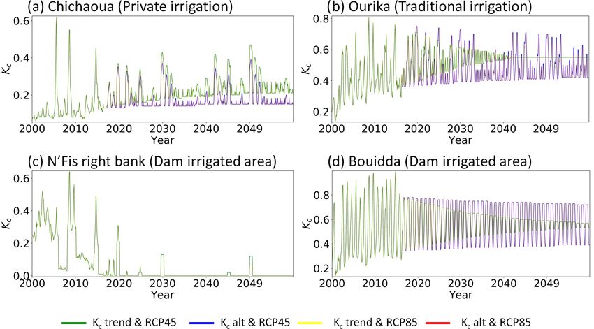
638                                                                M. Le Page et al.: Projection of irrigation water demand

subterranean water is overused to satisfy the growing water        implications of current trajectories as well as the options for
demand. In recent years, overexploitation of groundwater has       action (Raskin et al., 1998). Scenarios are therefore halfway
been facilitated by technological inventions, affordable cost      between facts and speculations in terms of complexity and
of exploitation, and weak monitoring by authorities (MED-          uncertainty (van Dijk, 2012). They are commonly used as a
EUWI working group on groundwater, 2007). The overex-              management tool for strategic planning and for helping man-
ploitation of aquifers can be observed in different countries      agers strengthen decision-making.
over the Mediterranean watershed (Custodio et al., 2016; Le           Various studies (Arshad et al., 2019; Lee and Huang, 2014;
Goulven et al., 2009).                                             Maeda et al., 2011; Schmidt and Zinkernagel, 2017; Tanasi-
   To satisfy the continuous increase in food demand associ-       jevic et al., 2014; Wang et al., 2016) have addressed the es-
ated with population growth, the agricultural sector has been      timation of irrigation water requirement (IWR) of a region
asked to pursue its already initiated process of conversion        with an approach close to Eq. (1). A simplified balance be-
toward agricultural intensification and above all towards a        tween crop evapotranspiration (ETc ) and effective precipi-
sharp increase in yields. This context goes hand in hand with      tation (Pe ) is computed for each crop i and multiplied by
the increase in food trade. The replacement of traditional         the corresponding irrigated area. ETc can be inferred from
crops by more financially attractive crops is already under-       the crop coefficient method (Kc ; Allen et al., 1998). Most
way (Jarlan et al., 2016). In the “growth” scenario (which         of the effects of the various weather conditions are incorpo-
is more or less the actual trend), presented by Malek et al.       rated into ET0 , which accounts for the water demand of a
(2018), the annual production of cultivated land increases         reference crop, while Kc mainly accounts for crop character-
by 40 % and the production of permanent crops increases by         istics. Kc varies according to four main characteristics: the
260 %. In the “sustainable” scenario, annual crop production       crop height, the albedo of the crop and soil, the canopy re-
and tree production increase by 30 % and 38 %, respectively.       sistance of the crop to vapor transfer (leaf area, leaf age and
As a consequence, irrigation water needs are expected to in-       condition, and the degree of stomatal control), and the evapo-
crease (Fader et al., 2016). The expansion and intensification     ration from soil, especially the soil exposed to solar radiation.
of tree crops will also further rigidify the demand for agricul-   Furthermore, as the crop develops, those different character-
tural water and increase the pressure on groundwater reser-        istics change during the various crop phenological stages. Kc
voirs (Jarlan et al., 2016) in order to keep tree crops alive      values and stage lengths, for typical climate conditions, are
during drought events (Le Page and Zribi, 2019; Tramblay           considered to be well known for many crops and have been
et al., 2020). This study is carried on in the Tensift basin in    compiled in the FAO (Food and Agriculture Organization)
Morocco, where the increase in the irrigated area and the in-      look-up tables.
tensification of irrigation during recent decades have caused
                                                                            n
a long-lasting drop in the groundwater table (Boukhari et                   X
                                                                   IWR =      (ETci − Pe ) · Areai
al., 2015). A multimodel analysis of the area over the period
                                                                            i=1
2001–2011 (Fakir et al., 2015) has shown that the groundwa-                 n
ter falls from 1 to 3 m/year and that the cumulated ground-
                                                                            X
                                                                        =         Kci · ET0 − Pe · Areai                        (1)
water deficit in 10 years (about 100 hm3 /year since 2001) is               i=1
equivalent to 50 % of the reserves lost during the previous
40 years. Among the main causes of this depletion is a re-            This approach is also a very convenient way to account for
duction and higher irregularity of precipitation (Marchane et      both climate and crop changes. On the one hand, Pe and ET0
al., 2017) for crop growth and groundwater recharge, a re-         are obtained from meteorology or climatology. On the other
duction of snow water storage (Marchane et al., 2015), an in-      hand, Kc values and stage lengths are taken from the tables.
crease and intensification of irrigated areas, and a progressive   Most of the work consists of evaluating the future irrigated
conversion to arboriculture due to national strategy. Since        area of each crop and assessing the impact of more efficient
irrigation relies increasingly upon groundwater abstraction,       irrigation techniques.
questions are inevitably raised concerning the future of local        There is a significant amount of literature about the esti-
agriculture and groundwater.                                       mation of land use and land cover changes (Mallampalli et
   Therefore, in regions where the cropping density and sur-       al., 2016; Noszczyk, 2018), with various techniques to esti-
face area of irrigated areas are growing strongly (see, for ex-    mate or predict them. Many land cover change approaches
ample, the cases of China and India; Chen et al., 2019), it is     are based on the transition probability that was introduced
necessary to make projections of the irrigation water demand       by Bell (1974) and have been eventually connected to cellu-
with the actual trend in order to build alternative scenarios.     lar automata to account for geographical interrelationships
In their review, March et al. (2012) defined scenario analy-       (Houet et al., 2016; Marshall and Randhir, 2008). A very
sis as “internally consistent stories about ways that a specific   interesting technique has been to combine the top-down
system might evolve in the future. Narrative scenarios are         (demand-driven) and bottom-up (local conversion) processes
plausible accounts of the future rather than forecasts”. Narra-    of land cover change by proceeding to a simplification of lo-
tive scenarios also help identify the drivers of change and the    cal processes (van Asselen and Verburg, 2013; Verburg and

Hydrol. Earth Syst. Sci., 25, 637–651, 2021                                          https://doi.org/10.5194/hess-25-637-2021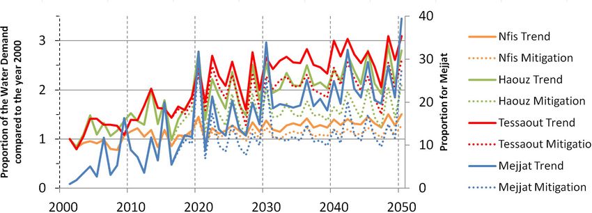
M. Le Page et al.: Projection of irrigation water demand                                                                        639

Overmars, 2009). Despite a huge bibliography both in cli-           In the Discussion section, other paths are discussed, in par-
mate change and land cover change, scenario analysis over           ticular those which are related to irrigation management.
the past 25 years has mostly focused on climate change pro-
jections, while the impact on land use and land cover has
been neglected. Titeux et al. (2016) found that only 11 %           2     Study site and data
of the 2313 studies analyzed have included both land cover
                                                                    2.1    Study area: the Haouz Plain in Morocco
and climate changes. Also based on a large review, March
et al. (2012) have called this a “hegemony” of climate as a         The study area includes the Haouz Plain, underlain by a large
driver of change. Furthermore, the implementation of land           Plio-Quaternary alluvial aquifer. It is located within the Ten-
cover change techniques appears to be tedious and does not          sift watershed in southern Morocco around the city of Mar-
account for the intensification of cropping patterns. The mo-       rakech (Fig. 1). The plain is bordered to the south by the
tivation of the present work is to take into account both land      High Atlas range. The High Atlassian watersheds that peak
cover change and crop intensification in future scenarios of        at 4167 m a.s.l. receive about 600 mm/yr of precipitation of
irrigation water demand, taking into account the impact of          which a major portion falls as snow; 25 % of the stream-
climate change.                                                     flow is generated by snowmelt (Boudhar et al., 2009). The
   The hypothesis is that the dynamics of land use change           plain, which is located at altitudes ranging between 480 and
and intensity of the cropping patterns (hence irrigation wa-        600 m a.s.l., has a semiarid climate (rainfall of 250 mm/yr
ter demand) can be reduced to a synthetic monthly Kc time           and potential evapotranspiration of 1600 mm/yr) with mild,
series for every irrigated area of the studied region. Each syn-    wet winters and very hot and dry summers. Irrigation is es-
thetic time series would then account for the spatial variabil-     sential for good crop development and yield. The so-called
ity of cropping patterns inside each irrigated area. Unless no      “traditional” areas (purple), which originally received wa-
sudden change occurs, a statistical model accounting for the        ter from the Atlassian wadis, are more and more depen-
monthly trend of Kc , the impact of rainfall, and the effect of     dent on groundwater. The areas irrigated from lake reservoirs
saturating the land cover with tree crops should give an ac-        (green) receive water from the Lalla Takerkoust reservoir, the
curate fit that would allow for extrapolating into the next few     Moulay Youssef reservoir, and also from the Hassan I reser-
decades. As the synthesis of Kc for separated irrigated areas       voirs through a 140 km canal called the Rocade Canal. The
would also decrease substantially the amount of information         rest of the irrigation water comes from the groundwater.
compared to a land cover approach, some information, like
the amount of tree crops, should be retrieved back from the         2.2    Data
time series. This approach would prevent the need for tedious
land cover classifications and reduce the difficulty of work-       In order to compute the crop water demand, regional climate
ing with discrete values for developing future scenarios.           model (RCM) simulations over the Mediterranean region
   The objective of this study is to produce two scenarios of       from the Med-CORDEX initiative (https://www.medcordex.
irrigation water demand for the different irrigated areas of        eu (last access: 1 January 2017); Ruti et al., 2016) were uti-
the Tensift watershed in Morocco. One is the trend and the          lized to provide future values of near-surface atmospheric
other one is an alternative scenario derived from a narrative       variables, namely the 2 m air temperature and total precipita-
scenario. To do so, a method for simulating and extrapolat-         tion. RCM results that are from two contrasting greenhouse-
ing Kc is proposed and is tested for the 2000–2016 period.          gas concentration RCP (Representative Concentration Path-
The future time series of Kc is used with climate change sce-       way) trajectory scenarios were selected: the RCP4.5 sce-
narios to obtain an estimate of future irrigation demands. As       nario, which represents the optimistic scenario for CO2
the strategy of irrigation for tree crops is treated very differ-   emissions (a stabilization of emissions) and the RCP8.5
ently from annual crops in the Tensift watershed, the yearly        (increasing emissions). Simulations from Centro Euro-
percentage of tree crops is also retrieved from the Kc time         Mediterraneo sui Cambiamenti Climatici (CMCC), Météo-
series.                                                             France (CNRM), and IPSL-Laboratoire de Météorologie Dy-
   The content of the article is separated into four parts and a    namique (LMD) were used in the current study. The three
conclusion. The first part describes the study area and the         RCMs give a good representation of the spread typically
dataset. The methodology is then detailed in three parts:           found in such simulations. The so-called “delta-change” or
(1) Kc time series are obtained from remote sensing observa-        perturbation method (Anandhi et al., 2011) was used to
tions for the observation period, (2) a model is constructed to     downscale the RCM data using the Global Soil Wetness
project the IWR based on simulating the evolution of Kc and         Project Phase 3 forcings (GSWP3: http://hydro.iis.u-tokyo.
integrating climate change, and (3) an alternative scenario is      ac.jp/GSWP3, last access: 1 January 2017) as the refer-
built from the trend to reflect a narrative scenario built by lo-   ence historical data. Statistical scores (bias and daily correla-
cal water managers. In the Results section, the performance         tion coefficients) were computed between the GSWP3 prod-
of the model and its ability to make projections are analyzed.      uct and 11 SYNOP (surface synoptic observations) stations
The alternative scenario is compared to the simulated trend.        over northwest Africa over the 1981–2010 period. GSWP3

https://doi.org/10.5194/hess-25-637-2021                                            Hydrol. Earth Syst. Sci., 25, 637–651, 2021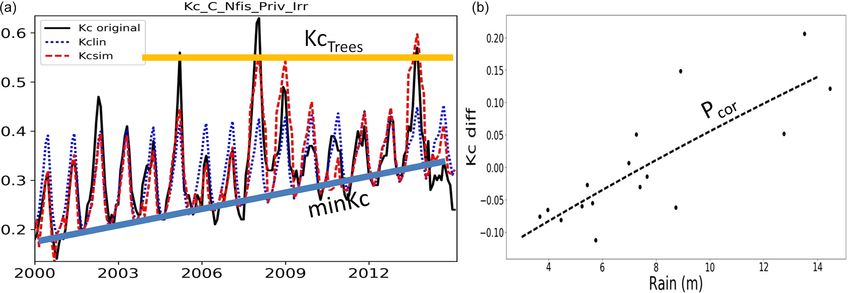
640                                                                       M. Le Page et al.: Projection of irrigation water demand

Figure 1. The Haouz-Mejjat aquifer is located within the Tensift watershed (gray) and separated into four subareas. The most important
traditional and dam irrigated areas are shown on the map. The N’Fis area is a mix of traditional and modern irrigation. All of these areas also
use groundwater, but outside them, the irrigated areas (private irrigation) rely exclusively on groundwater.

well represents the variability of temperature, relative humid-              For generating vegetation time series, we used the
ity, and total precipitation. The correlation coefficients com-           MOD13Q1 Collection 6 product (Didan, 2015), which pro-
puted between both monthly time series are 0.99, 0.87, and                vide 16 d composite series of Normalized Difference Vege-
0.74 for temperature, relative humidity, and precipitation, re-           tation Index (NDVI) from the Moderate Resolution Imaging
spectively. Standard deviations are quite small for the three             Spectroradiometer (MODIS) at a spatial resolution of 250 m.
variables (0.01, 0.03, and 0.12, respectively). At the daily              This product is computed from atmosphere-corrected (Jus-
time step, GSWP3 well represents the day-to-day temper-                   tice et al., 2002), daily bidirectional surface reflectance ob-
ature variability and especially the relative humidity. How-              servations, using a compositing technique based on product
ever, GSWP3 has more errors in terms of the daily evolution               quality (Wan et al., 2015). We used the 16 d composites to
of precipitation (r = 0.08, SD = 14.6). In semiarid regions,              reduce cloud coverage. The data have been compiled for the
where precipitation is infrequent and often convective, it is             period 2000–2016.
difficult to reproduce the precipitation events at the actual
time. In terms of bias, the absolute temperature and rela-
tive humidity values are close to that observed: 0.22 ◦ C and
0.54 %, respectively; meanwhile, precipitation is underesti-              3     Methodology
mated by approximately 10 % on average, but this bias is not
always consistent from one station to another. The 0.5◦ data              3.1    Kc assessment from remote sensing time series
were resampled to a resolution of 1 km, applying a correction
of altitude between the GSWP3 geopotential and a digital el-              Neale et al. (1990) proposed to estimate the Kc coefficient
evation model (GTOPO30 available at https://www.usgs.gov,                 from vegetation indices obtained from remote sensing im-
last access: 1 January 2017) for air and dew point tempera-               agery. In this work, we have been using empirical linear
tures.                                                                    equations where the slope (a) and intercept (b) have been
   The resulting downscaled and rescaled (to 1 km resolu-                 previously calibrated for common crop type in local field
tion) dataset of meteorological variables (rain, temperature,             experiments (Duchemin et al., 2006; Er-Raki et al., 2007,
wind speed, relative humidity and global radiation) extends               2008):
from 2000 to 2050.
                                                                          Kc,sat = a · NDVI + b.                                           (2)

Hydrol. Earth Syst. Sci., 25, 637–651, 2021                                                   https://doi.org/10.5194/hess-25-637-2021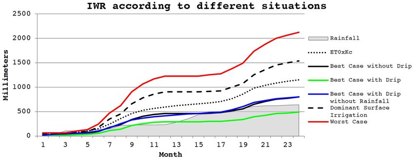
M. Le Page et al.: Projection of irrigation water demand                                                                      641

   Equation (2) accounts for combined evaporation from the             Py was best modeled using a second-degree polynomial
soil and transpiration from the crop in a very simple way, but         according to Eq. (6). An example of this fit is given on
as no water balance is performed, several assumptions must             the right side of Fig. 3.
be kept in mind. (1) The extra evaporation due to wetting
events (rainfall, irrigation) is not computed but is assumed to
be represented in the calibrated NDVI / Kc,sat relationship,           1Kc (y) = Kc,lin (y) − Kc,sat (y) ,                    (4)
which is related to the precipitation of the year used for cali-            Xmar
bration. The inability of this method to increase the evapora-         Py =      Pm ,                                         (5)
tion part of evapotranspiration when frequent small rainfall                 m=sep
events occur should be assessed and corrected for, either at           Kc,cor Py = a2 · Py2 + b2.Py + c2 (where a2, b2,

the level of the ETc computation or in the Pe computation.
                                                                             and c2 are fitted to 1KcM for Py ).              (6)
(2) The lower evaporation due to a reduction of the wetted
fraction characteristic of micro-irrigation is not taken into ac-
                                                                    3. In the third stage, the tree crops and their preservation
count. (3) The crop water stress is not taken into account in
                                                                       were taken into account. In fact, in semiarid Mediter-
this calculation, as the time step of 1 month causes this to be
                                                                       ranean regions, evergreen tree orchards (olive, citrus)
quite complex to represent. However, significant stress may
                                                                       are the major crops responsible for green vegetation in
impact the evolution of the NDVI signal. The approach of
                                                                       the dry season of summer, although the cultivation of
estimating Kc,sat is displayed in the light gray area in Fig. 2.
                                                                       summer vegetables is also possible. In the Tensift re-
                                                                       gion, orchards come first in order of preference for wa-
3.2   Trend projection of Kc
                                                                       ter allocation in agriculture, especially in dry years. The
The simulation of Kc was carried out as follows: a linear              aim is to preserve the tree crops from drought. To en-
adjustment from the original Kc,sat is obtained from remote            sure that the tree crop area would not be reduced from
sensing; secondly, this first guess is corrected according to          one year to the next, the minimum Kc,sim was forced
the rainfall of the year; finally, a correction is made accord-        to not run in the opposite direction to the trend slope
ing to the percentage of tree crops. Figure 3 illustrates the          (it will not be reduced when the trend is growing and
quantities used to perform this calculation. The four steps            inversely). In other words, the yearly rate of minimum
detailed below were reproduced for each of the 29 irrigation           Kc is growing; a new value is ensured to be greater or
areas of the study.                                                    equal to the minimum value of the previous year. Fi-
                                                                       nally, to ensure that the resulting synthetic Kc would be
  1. The first step was to perform a linear adjustment (Eq. 3).        in line with the proportion of trees in the irrigated area,
     For each month M, of the year y, a linear least-squares           the percentage of tree crop has been obtained during the
     fit was made to the Kc,sat values for all years in the se-        dry season when it is assumed that there is no other crop
     ries; thus, we obtained a set of 12 monthly regression            than trees:
     equations for Kc,sat as a function of the year. These 12
     linear regressions thus formed the time series Kclin . An         % Trees(y) = minKc(y)/Kc,Trees ,                       (7)
     example is plotted in blue in Fig. 3:                             where minKc is the minimum Kc,sim for the hydrolog-
                                                                       ical season (see the blue line in Fig. 3), and Kc,Trees is
      Kc,linM (y) = a1M y + b1M (where a1 and b1
                                                                       the maximum Kc for the tree crop considered (see the
             are fitted to Kc,satM (y) for M ∈ [1, 12]).     (3)       orange line in Fig. 3). For the study area, in which olive
                                                                       trees are the dominant tree crop, Kc,Trees has been set
  2. The second step consisted of correcting the first approx-         to 0.55 (Allen et al., 1998). The potential maximum Kc
     imation of Kc,lin for the impact of rainfall. In this semi-       of each year (maxKc) was computed with the weighted
     arid region, sowing and the development of the vege-              sum as follows:
     tation depend very much on the time distribution and              maxKc(y) = Kc,max · (1 − % Trees(y)) + Kc,Trees
     accumulation of rainfall during the agricultural season.
     We chose March as the month most representative of                           · % Trees(y),                               (8)
     these interannual differences (Le Page and Zribi, 2019).          where the non-tree-crop area has a maximum Kc of
     On the one hand, we calculated the difference in Kc               Kc,max , which was set according to winter wheat as in
     (1Kc ) between the observation (Kc,sat ) and the linear           Allen et al. (1998). Winter wheat is a dominant crop of
     regression (Kc,lin ) in the month of March as in Eq. (4).         the study area, and its maximum Kc (1.15) is among the
     On the other hand, the rainfall accumulation Py was               highest known.
     summed between September and March according to
     Eq. (5). This has been done for each year from 2000 to         4. The final estimate of monthly Kc (Kc,sim ) integrated the
     2016. We found that the relationship between 1Kc and              linear trend, the yearly variation due to rainfall, and the

https://doi.org/10.5194/hess-25-637-2021                                          Hydrol. Earth Syst. Sci., 25, 637–651, 2021
642 M. Le Page et al.: Projection of irrigation water demand
Figure 2. Processing steps flowchart. The light gray area of the flowchart was presented in Le Page et al. (2012). The calculations on Kc are
performed on 29 irrigated areas. The input data are indicated in gray boxes. Variable extraction is indicated by a square box. Processing steps
(and their results) are indicated by boxes with beveled corners. The indications between parentheses show the temporal, spatial, and scenario
resolutions. The scenario generation described in this article is indicated in dark gray.
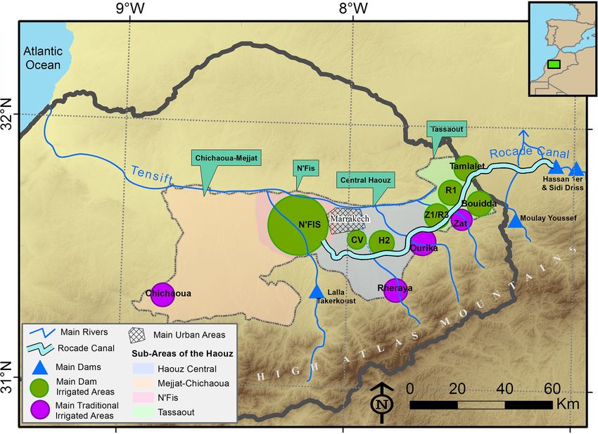
Figure 3. (a) Quantities used to perform the simulation. The example illustration on the left depicts the synthetic Kc of the N’Fis private
area where a mix of tree crops (olive, orange, apricot) and cereal crops (mainly wheat) are cultivated. The peak occurs during March and
April when cereal crops are at their maximum development; the valleys correspond to the summer months when there are no seasonal crops.
The three curves are the Kc time series obtained from remote sensing processing (solid line), the linear estimation (Kc,lin , Eq. 3, dotted blue
line), and the estimation corrected with rainfall (Kc,sim , Eq. 6, dashed red line). Kc,Trees has been set to 0.55 in Eq. (8), and minKc is the
yearly minimum of Kc on Kc,sim . (b) The fitted correction curve of Kc according to the cumulated rainfalls (Pcorr ) is almost linear in this
example.
limitation due to the coverage of tree crops (Eq. 9). this sum did not exceed the potential maximum Kc
(maxKc, Eq. 8). It was also ensured that it did not go
Kc,simM (yP ) =max[min Kc,linM (y) + Kc,cor (P ) , below the Kc of bare soil (Kc,min = 0).
maxKc(y)) Kc,min ], (9)
The set of Eqs. (3) to (9) together model the future trend
where the variability of Kc due to yearly rainfall (Kc,cor ) of Kc . The water demand was then computed from Eq. (1),
was added to the first guess Kc,lin . It was ensured that where ET0 incorporated the weather conditions, and in par-
Hydrol. Earth Syst. Sci., 25, 637–651, 2021 https://doi.org/10.5194/hess-25-637-2021M. Le Page et al.: Projection of irrigation water demand 643
ticular the modifications of temperature predicted by the ter pumping; (2) the conversion of surface irrigation to drip
RCPs. irrigation; (3) an intensification of arboriculture; and (4) an
The performance of the model has been assessed using abandonment of irrigated cereals for vegetable crops. How-
different sampling techniques to obtain calibration and val- ever, neither the plans nor the interviews specify the inten-
idation datasets. First, calibration years are selected to be sity or locations of these changes. Here, we do not address
equally spaced along the time axis: 1 out of every 2 years all of the measures considered, only those concerning land
(8 years), 1 out of every 3 years (6 years), and 1 out of ev- cover changes. A reduction in the rate of increase of olive
ery 4 years (4 years) of calibration. For the “every 2 years” tree areas by 50 % is expected to begin in 2021. At the same
sampling, there were two sets of calibration years; for the time an intensification due to intercropping and the replace-
“every 3 years” sampling, there were three calibrations sets, ment of traditional Moroccan Picholine (100 to 200 trees per
and so on. The three different versions of the model were hectare) by Spanish Arbequina with a density of 1000 trees
run for the different combinations of calibration and valida- per hectare will take place. This is correlated with the ex-
tion datasets. The versions tested were the linear fit (Kc,lin ), pected production increase of 27 %. The fate of citrus trees
the linear fit with rain correction (Kc,cor ), and then with tree is less clear. The recent trend is a strong expansion; however,
correction (Kc,sim ). The performance indicators were aver- the plan expected a stabilization of citrus orchards due to the
aged for each group (1/2, 1/3, 1/4). The years have also been lack of water especially in the western part of the basin. Fi-
separated into two groups: years with less precipitation are nally, a progressive reduction of cereal crops (−722 ha/yr) is
called the “dry years” (2001, 2002, 2005, 2007, 2008, 2011, expected. Here, we proposed to only modify the main trend
2012, 2014, 2016) and the rest are called “wet years”. Three of the Kc curve in order to represent the idea of a pause in
statistical metrics have been computed: the determination co- crop-cover expansion. The set of equations to simulate the
efficient r 2 (Eq. 10), the root mean squared error (RMSE, bending of the curve are the following:
Eq. 11), and the standard deviation of error SE (Eq. 12):
r a10 = a1 · bc ,
2 Cov(X, Y ) b10 = (a1 · bc + b1) − yc a10 ,
r = , (10)
σXσY
s Kc0 ,sim = a10 · Kc,sim + b10 . (13)
Pn 2
1 (X − Y )
RMSE = , (11) A new slope (a10 ) and intercept (b10 ) were computed ac-
n
sP cording to a bending coefficient (bc ) and applied for the de-
n
1 (X − Y ) sired years where yc is the beginning year of the bending.
SE = . (12)
n The bending coefficient was expressed as a percentage.
In order to demonstrate the feasibility of applying scenar-
3.3 Alternative evolution of Kc ios with this model, it was determined that the introduction
of two bending points to the trend scenario (Eq. 13) gave a
The set of Eqs. (3) to (9) was used as a basis for simulat- good representation of the vision of the narrative scenario
ing the long-term trend of Kc . The coefficients a1 and b1 of (−50 % on the trend in 2020 and another −50 % by 2040).
Eq. (3) were fitted with the data from the entire time series. Note that the narrative scenario did not give a detailed view
The parameters a2, b2, and c2 of Eq. (6) were fitted using of the changes, so those coefficients have been applied uni-
the rainfall data taken from the downscaled climate scenario. formly to the 29 irrigated areas.
The system of equations allows for the consideration of
various possibilities for “bending the curve” (Raskin et al.,
1998), which here means modifying the trend of the crop- 4 Results
ping scenario: (1) the parameters a1 and b1 in Eq. (3) can
be modified to account for an overall change in the trend; (2) 4.1 Performance of the simulated Kc,sim
the coefficients a2, b2, and c2 in Eq. (6) can be modified to
account for the influence of cumulative rainfall. (3) The hy- Figure 4 shows the three statistical metrics of the fit for dif-
pothetical law that determines that the rate of change in tree ferent calibration groups. The calibration is computed against
coverage always has the same sign could be relaxed so that a a subset of the 16 years, where one-half (1/2) means 8 cal-
decrease of tree coverage could be possible. ibration years for 8 validation years, one-third (1/3) means
As the status of the Haouz aquifer is becoming criti- 5 calibration years for 11 validation years, and one-quarter
cal, alternative trend scenarios have been proposed by the (1/4) means 4 calibration years for 12 validation years. r 2
Tensift Hydraulic Basin Agency (Agence du Bassin Hy- values were generally located around 0.5, which indicates an
draulique du Tensift) with the support of GIZ (Gesellschaft average fit, but they decreased when the calibration set size
für Internationale Zusammenarbeit) (ABHT GROUP AG – decreased. RMSE ranged between 0.1 for half of the cali-
RESING, 2017). The main drivers defining these changes in- bration years to 0.17 for the corrected methods for only four
clude (1) an expansion of irrigated areas through groundwa- calibration years. It must be noted that the Kc,sim and Kc,cor
https://doi.org/10.5194/hess-25-637-2021 Hydrol. Earth Syst. Sci., 25, 637–651, 2021644 M. Le Page et al.: Projection of irrigation water demand
The performance of the algorithm may be summarized as
follows. The simple linear relationship provided an average
approximation. The rainfall correction improved the average
performance if the calibration years were representative of
the validation years; elsewhere, it worsened the prediction.
There was no visible effect of the tree correction during the
period of time when observations were available. The bound-
ing constraint was basically not reached. Finally, the model
results were much better when the calibration years were
representative of the rainfall variability (wet and dry years).
Given that the remote sensing dataset was processed for the
2000–2016 period (16 years), the performance of the predic-
tion at the 2050 horizon should be comparable to the 1/3 test:
Figure 4. Performance indicators (r 2 , RMSE, SE) for the three vari- r 2 = 0.5, RMSE = [0.1–0.14], and SE = [0.02–0.03].
ations of the model (Kc,lin , Kc,cor , Kc,sim ) as a function of the
splitting strategy for determining the calibration/validation dataset. 4.2 Evaluation of the trend and alternative evolution
under climate change
versions lower the performances regarding RMSE when only Figure 6 shows examples of the extrapolation of Kc for four
1/3 or 1/4 of the years is used. This is also true for the dry contrasted irrigated areas, with the trend and alternative Kc
calibration years, which is explained by the fact that the rain- scenarios and RCP4.5 and RCP8.5 climatic scenarios. The
fall correction (Kc,cor ) needs a good representativeness of ex- region of private irrigation in Mejjat was all but covered with
treme cumulative precipitations. drylands until the early 90s. A boom of groundwater ex-
The trajectory of each irrigated sector can be very dif- ploitation has provoked the development of irrigated areas.
ferent, according to its mix of crop, cropping intensity, and Kc spikes in the rare wet years, but most of the time, the am-
evolution. Figure 5 shows an example of this diversity with plitude of the signal is very small, showing that the area is
four contrasted irrigated areas. The figure also shows the cal- mostly composed of bare soils and tree crops. The trend pro-
ibrated and original time series of Kc when the calibration jection predicts that the Kc will tend toward an average of 0.2
is carried out over the entire time series. The Chichaoua pri- by the year 2050, which means the impact of irrigation will
vate area gave the worst result. As can be seen, the low r 2 be much greater than at the beginning of the 21st century.
was mainly due to the poor distribution of the data at very The alternative Kc greatly reduced the trend and stabilized
low Kc . It is very likely that most of the area was not irri- around 0.15. Ourika is an irrigated area located at the pied-
gated continuously during the whole study period. The N’Fis mont of the Atlas mountains. This area has traditionally re-
right bank is located on the outskirts of the city of Marrakech, lied on spate irrigation from the Atlas wadis fed by snowmelt.
under high urban pressure. The negative trend was well pre- This area is also located over the Haouz aquifer where it ben-
dicted and the correlation score was satisfactory (r 2 = 0.77) efits from recharge from below-river flows. The full coverage
despite the probably erroneous pause in the original Kc data with tree crops was attained around 2040 in the Ourika area.
in 2006 and 2007. The Ourika traditional area is located Therefore, the synthetic Kc of this area is controlled by the
at the outlet of the Ourika River. The scores were average maximum Kc value of Eq. (8), which was set equal to the Kc
(r 2 = 0.646, slope = 0.747). The general growing trend was of olive trees (0.55), which is the dominant tree crop of this
reproduced, especially for the base of the curve. The max- region.
imum and minimum Kc values simulated with the amount On the alternative trajectory, Kc is less saturated, mean-
of annual rainfall were generally accurate, except for the 2 ing that there is still a place for annual crops. As stated ear-
years (2002 and 2003). Those are extremely dry years where lier, the N’Fis right bank irrigated area, which is located near
rainfed cereals could not develop, and there were strong ir- Marrakech, already had a trend toward the disappearance of
rigation restrictions. The Bouidda district is an area irrigated irrigated crops. The two projections maintained the Kc level
by the Moulay Youssef reservoir in the eastern part of the near zero except for wet years. The Bouidda irrigated area
study area. It obtained one of the best scores (r 2 = 0.863). in the Tessaout (also spelled Tassaout) region follows a trend
The area is dominated by cereals, which explains the typical of reconversion toward tree crops without a trend of cropped
seasonal Kc curve. The increase in permanent tree crops was area development, which is almost fulfilled by 2050. In the
well simulated at the baseline. There was also an intensifica- alternative scenario, this trend was controlled, and the area
tion of cereal crops that increased the peaks at the end of the maintained a mix of annual and tree crops.
study period. The lower Kc years, 2006 and 2007, were well In those four examples, the climatic scenarios of rainfall
simulated. The very dry year 2001 was simulated but did not only had a minimum impact on the Kc time series.
reach the minima observed in the original curve.
Hydrol. Earth Syst. Sci., 25, 637–651, 2021 https://doi.org/10.5194/hess-25-637-2021M. Le Page et al.: Projection of irrigation water demand 645 Figure 5. Examples of Kc simulations compared to the original time series for four selected areas. Figure 6. Examples of long-term simulation of Kc in four different irrigated areas with the trend and alternative scenarios of Kc and the RCP4.5 and RCP8.5 climatic scenarios. Figure 7 shows the relative evolution of water demand lation and has not been plotted in Fig. 7. However, we must compared to the year 2000 and the expected impact of the keep in mind that if climate change only slightly impacts the “bending” effect for the four different planning areas in the water demand, it will probably reduce the water supply, be- watershed (see Fig. 1). The expected temperature increase cause the runoff decrease will reduce the surface water avail- between RCP4.5 and RCP8.5 is about 1 ◦ C by 2050, leading able for irrigation (snowmelt, runoff, reservoirs). The area to a 2 % difference in yearly ET0 . The impact on irrigation equipped for irrigation (AEI) also remains unchanged while water demand is therefore minimal by the end of the simu- the actual irrigated area may change inside those AEIs. Those https://doi.org/10.5194/hess-25-637-2021 Hydrol. Earth Syst. Sci., 25, 637–651, 2021
646                                                                      M. Le Page et al.: Projection of irrigation water demand

Figure 7. Trend and alternative scenarios for irrigation water demand in the four planning areas of the Tensift with RCP8.5.

simulations showed that each area had it’s own dynamics                 range (2050) which resulted in a difference of only 1 ◦ C
(bearing in mind that subareas also had their own dynam-                and almost no difference in precipitation over the study re-
ics). The Mejjat area, which was mostly unexploited in the              gion. It should be noted that the predicted impact of climate
year 2000, has been experiencing significant growth since.              change on precipitation is more variable in space and less
We can also see that by 2040 the demands tend to stabilize in           certain than that for temperature. It also may be due to the
the trend lines owing to the saturation effect of the irrigated         absence of the impact of including increasing atmospheric
areas. In the alternative scenario, the reduction in the agricul-       CO2 concentration prescribed by the RCP scenario in our ap-
tural development rate stabilizes at a lower level. The N’Fis           proach. Different strategies are possible. For example, Fares
area showed the lowest increase, and the modeled trend to-              et al. (2015) proposed a modification of the ratio bulk re-
ward a flat line showed that the area will be fully dominated           sistance over stomatal resistance rs /ra in the ET0 equation
by tree crops by 2050. The Haouz and Tessaout areas showed              based upon the CO2 emission scenario. The low impact of
the most significant increases in irrigation water demand, as           RCP scenarios could also be explained by the fact that the
it almost tripled during the 50 years of simulation. However,           potential decrease in the annual crop growth cycle duration
the alternative scenario mitigated these increases.                     associated with temperature rise is not represented. Accord-
                                                                        ing to Bouras et al. (2019), the reduction of the cycle can
                                                                        reach 30 % at mid-century under the RCP8.5 scenario for
5   Discussion                                                          wheat in the study region. Similar results were obtained with
                                                                        the ISBA-A-gs model (Calvet et al., 1998) when studying the
The proposed method allowed for projecting irrigation wa-               impact of climate change on Mediterranean crops (Garrigues
ter demand by including both the anthropogenic and climatic             et al., 2015). It is also interesting to note that if the water
vector of changes. The output is given for the next 30 years            demand for seasonal crops is reduced with the crop cycle
for each demand site at the monthly time step, which is a               duration, the yield may also be affected by extreme tempera-
timescale that is commonly used by water planners. Various              tures (Hatfield and Prueger, 2015) so that the trend might be
improvements to the method have been identified. (1) Kc was             affected in order to reach the production objective.
determined by a precalibrated linear relation to the NDVI                  Finally, the assessment of irrigation water demand should
time series. If an actual evapotranspiration product (see, for          also take into account different losses at the system level
example, Xu et al., 2019) would be available for the whole              (storage, transportation, and operating losses) and at the plot
period of study and at a resolution compatible with the size            level (deep percolation and runoff). The future evolution of
of the irrigated areas, Kc could be determined by comput-               the irrigation framework toward more efficient systems such
ing the ratio between actual evapotranspiration products and            as drip irrigation could also be considered using Eq. (14).
reference evapotranspiration. (2) The gridded data were syn-            This equation of gross irrigation water requirement (IWRG
thesized at the monthly time step for each irrigated area, by           expressed in m3 ) is rewritten from Eq. (1):
computing arithmetic averages, which resulted in a loss of
                                                                                        AEI ϕET0 Kc − αP
information. If needed, other statistical indicators, such as           IWRG = 1/σ                       ,                          (14)
the dominant land cover of the irrigated area, could be kept                            10       β
for further analysis. (3) The main temporal trend was fitted            where AEI (hectares) is the area equipped for irrigation. The
with monthly linear regressions (Eq. 3). The degree of the              system efficiency σ is the ratio of water delivered upstream
regression could be easily adapted if the model does not fit            to the water that is distributed to the plots (Blinda, 2012).
adequately with the observations.                                       The coefficient α produces the efficient rainfall similar to that
   The very low difference in impact between the two RCP                proposed by USDA-SCS (1970). The coefficient ϕ is used to
scenarios is interesting. It can be explained by the short time         account, in a simple manner, for a reduction of evapotran-

Hydrol. Earth Syst. Sci., 25, 637–651, 2021                                                 https://doi.org/10.5194/hess-25-637-2021
M. Le Page et al.: Projection of irrigation water demand 647
Figure 8. IWRG according to different efficiencies for 2 years of example (September 2011 to August 2013) in the case of an irrigated
wheat. In the best case without drip curve, all coefficients are set to one except the efficient rainfall, which is set to a classical 0.75 (σ =1,
ϕ = 1, α = 0.75, β = 1). In the best case with drip, The σ coefficient of localized irrigation is set to 0.7 (σ = 1, ϕ = 0.7, α = 0.75, β = 1).
The best case with drip but without taking into account rainfall simulates the irrigation practice done to prevent soil leaching (σ = 1, ϕ = 0.7,
α = 0, β = 1). The dominant surface irrigation simulates an irrigated sector where surface (gravity) irrigation dominates (α = 0.5) and where
the system performance is good (σ = 0.9) (σ = 0.9, ϕ = 1, α = 0.9, β = 0.5). The worst case depicts an irrigated sector with low irrigation
efficiencies (σ = 0.75, ϕ = 1, α = 0.75, β = 0.5).
spiration due to micro-irrigation. β is the effective irrigation climate scenarios (RCP4.5 and RCP8.5) were introduced into
coefficient; it is low for surface irrigation (50 %–70 %) and the trend as alternative scenarios. The local anthropogenic
close to 100 % for drip irrigation. The behavior of Eq. (14) scenarios of irrigation water demand had rapidly changing
is displayed in Fig. 8 for 2 sample years (September 2011 to dynamics and were spatially contrasted. On the contrary, the
August 2013) for the R3 irrigated sector where wheat is the difference in impact between the two climate change sce-
dominant crop. According to those different efficiency con- narios appeared to be very small over the next 30 years, al-
figurations, IWR can vary from single to more than quadru- though the impacts of atmospheric carbon concentration on
ple between the ideal best and the worst situation. However, stomatal controls of the plant were neglected. Finally, the dis-
note that those configurations are theoretical. The best case cussion showed that the approach could easily be combined
with drip irrigation is virtually unachievable in real condi- with irrigation efficiency scenarios. The conjunction of the
tions. present approach with irrigation efficiencies would proba-
bly be a suitable combination for the modeling of water re-
sources management. The approach can be applied to other
6 Conclusions regions where there is a significant growth of irrigated ar-
eas. The MODIS products are available over all the globe, so
Owing to their inherent complexity, scenarios of agricultural the retrieval of a 20-year-long time series of crop coefficients
evolution based on interviews are very difficult to translate can be done anywhere. Different alternative techniques exist
into numbers (when and how much) and to represent spa- to retrieve Kc so that it is possible to switch between meth-
tially (where). The simple and flexible statistical approach ods. A caveat of using these data, however, is their relatively
proposed here is a possible solution for quantifying spatially low spatial resolution (250 m), which implies that some field-
distributed scenarios of agriculture evolution in the context of scale details might be missed or undersampled. The separa-
climate change and irrigated areas that are rapidly changing tion of the territory between different irrigated areas seems
owing to socioeconomic influences. This is the case for many adequate in particular when using a water allocation model.
Mediterranean areas like the Tensift watershed, which was The synthesizing algorithm is efficient and can be applied in
the case used for the current study. The performance of the different regions. The model itself is mainly linear, even if
model was acceptable in most irrigated areas, giving monthly it is corrected by yearly precipitation and an eventual satu-
correlation coefficients for Kc of up to 0.92 but with signif- ration due to the extension of tree crops. In other situations,
icant differences between the irrigated areas. It was shown for example, a late expansion of irrigated areas or where a
that the prediction performance of the model was a func- reduction of the expansion is already noticeable, it will be
tion of the length of the calibration period. With 16 years of necessary to switch to a nonlinear system. A simple ordinary
data (2000–2016), the prediction could only be done for two least square adjustment has been used to fit the coefficients,
other periods of 16 years (until 2050). In order to demon- but other more sophisticated techniques could be used. Those
strate the flexibility of the model for scenario building, a lo- different questions are being taken into account in the frame
cal scenario of water resource management was reinterpreted
to build an alternative scenario upon the trend scenario. Two
https://doi.org/10.5194/hess-25-637-2021 Hydrol. Earth Syst. Sci., 25, 637–651, 2021648 M. Le Page et al.: Projection of irrigation water demand
of the AMETHYST project over the Merguellil watershed in Competing interests. The authors declare that they have no conflict
Tunisia. of interest.
Code availability. Models or code generated or used during the Special issue statement. This article is part of the special issue
study are available from the corresponding author by request. “Changes in the Mediterranean hydrology: observation and mod-
eling”. It is not associated with a conference.
Data availability. Some of the data used during the study are
freely available in online repositories. (1) The datasets of the Med- Acknowledgements. We thank NASA for kindly providing us with
CORDEX RCP45 and RCP85 climate scenarios that have been used the TERRA-MODIS NDVI products and Hungjun Kim (The Uni-
are following: versity of Tokyo) for providing the atmospheric forcing data from
the Global Soil Wetness Project. We would also like to thank the
– CNRM/GAME RCP45 MEDCORDEX_MED-44_CNRM-
Med-CORDEX providers for making their regional climate data
CM5_rcp45_r8i1p1_CNRM-ALADIN52_v1, http://mistrals.
available. We are especially grateful to the Tensift Hydraulic Basin
sedoo.fr/?editDatsId=941 (Somot, 2013a);
Agency (ABHT) and the Haouz Agriculture Office (ORMVAH) for
– CNRM/GAME RCP85 MEDCORDEX_MED- making their data available for the integrated modeling. Finally, we
44_CNRM-CM5_rcp85_r8i1p1_CNRM-ALADIN52_v1 thank the AGIRE project for providing the tentative scenarios of the
http://mistrals.sedoo.fr/?editDatsId=938 (Somot, 2013b); Tensift watershed.
– CMCC RCP45 MEDCORDEX_MED-44_CMCC-
CM_rcp45_r1i1p1_CMCC-CCLM4-8-19_v1, https:
//mistrals.sedoo.fr/?editDatsId=1088 (Conte, 2013); Financial support. This research has been supported by the Agence
Nationale de la Recherche (AMETHYST, ANR-12-TMED-0006-
– CMCC RCP85 MEDCORDEX_MED-44_CMCC- 01), the Centre National pour la Recherche Scientifique et Tech-
CM_rcp85_r1i1p1_CMCC-CCLM4-8-19_v1, https: nique (SAGESSE, PPR/2015/48 , program funded by the Moroc-
//mistrals.sedoo.fr/?editDatsId=1135 (Conte, 2014); can Ministry of Higher Education), and the FP7 International Co-
– LMD RCP45 MED-44_IPSL-IPSL-CM5A- operation (CHAAMS, ERANET3-062). The Laboratoire Mixte In-
MR_rcp45_r1i1p1_LMD-LMDZ4NEMOMED8_v1, ternational TREMA (IRD, UCA) and MISTRALS/SICMED2 are
https://mistrals.sedoo.fr/?editDatsId=1116&datsId=1116& thanked for additional funding.
project_name=MISTRALS&q=lmd+rcp45 (Li, 2014a);
– LMD RCP85 MED-44_IPSL-IPSL-CM5A-
Review statement. This paper was edited by Gil Mahe and reviewed
MR_rcp45_r1i1p1_LMD-LMDZ4NEMOMED8_v1
by two anonymous referees.
https://mistrals.sedoo.fr/?editDatsId=1116&datsId=1116&
project_name=MISTRALS&q=lmd+rcp85 (Li, 2014b).
(2) The Normalized Difference Vegetation Index 16 days
L3 from MODIS/Terra (i.e., MOD13Q1) is available at
https://doi.org/10.5067/MODIS/MOD13Q1.006 (Didan, 2015), References
(3) The USGS DEM data (i.e., GTOPO30) are available at
https://doi.org/10.5066/F7DF6PQS (United States Geological ABHT GROUP AG – RESING: Plan d’action pour la convention
Survey’s Earth Resources Observation and Science (USGS EROS) GIRE Scénario tendanciel pour le bassin Haouz-Mejjat, available
Center, 1996). at: http://conventiongire.lifemoz-dev.com/wp-content/uploads/
The Global Soil Wetness Project Phase 3 dataset (i.e., GSWP3) sites/52/ftp/Rapports/PlanActionConventionEau2017web.pdf
(Dirmeyer et al., 2006) was provided by Hyungjun Kim from The (last access: 1 January 2018), 2017 (in French).
University of Tokyo (see Acknowledgements section). Allen, R., Pereira, L., Raes, D., and Smith, M.: FAO Irrigation and
The data used for deriving an alternative scenario are proprietary Drainage no. 56: Guidelines for Computing Crop Water Require-
or confidential in nature and may only be provided with restrictions ments, FAO, 1998.
by the Agence du Bassin Hydraulique du Tensift. Anandhi, A., Frei, A., Pierson, D. C., Schneiderman, E.
M., Zion, M. S., Lounsbury, D., and Matonse, A. H.:
Examination of change factor methodologies for climate
Author contributions. MLP analyzed and processed the satellite change impact assessment, Water Resour. Res., 47, W03501,
and meteorological data and proposed the model. LJ and AB su- https://doi.org/10.1029/2010WR009104, 2011.
pervised the work, reviewed the paper, and took part in critical dis- Arshad, A., Zhang, Z., Zhang, W., and Gujree, I.: Long-Term Per-
cussions. AB disaggregated the climate change forcings. YF partic- spective Changes in Crop Irrigation Requirement Caused by
ipated in the formulation of the research question and the writing Climate and Agriculture Land Use Changes in Rechna Doab,
of the paper. BB coordinated the work with the Tensift Hydraulic Pakistan, Water, 11, 1567, https://doi.org/10.3390/w11081567,
Basin Agency. LJ, SK, and MZ participated in the research of fund- 2019.
ing and reviewed the paper. All authors read and agreed with the Bell, E. J.: Markov analysis of land use change–an application of
article. stochastic processes to remotely sensed data, Socio Econ. Plan.
Hydrol. Earth Syst. Sci., 25, 637–651, 2021 https://doi.org/10.5194/hess-25-637-2021M. Le Page et al.: Projection of irrigation water demand 649 Sci., 8, 311–316, https://doi.org/10.1016/0038-0121(74)90034- Er-Raki, S., Chehbouni, a., Guemouria, N., Duchemin, B., Ezza- 2, 1974. har, J., and Hadria, R.: Combining FAO-56 model and ground- Blinda, M.: More efficient water use in the Mediterranean, Plan based remote sensing to estimate water consumptions of wheat Bleu, Valbonne, Plan Bleu Papers no. 14, ISBN 978-2-912081- crops in a semi-arid region, Agr. Water Manage., 87, 41–54, 35-3, 2012. https://doi.org/10.1016/j.agwat.2006.02.004, 2007. Boudhar, A., Hanich, L., Boulet, G., Duchemin, B., Ber- Er-Raki, S., Chehbouni, A., Hoedjes, J., Ezzahar, J., Duchemin, jamy, B., and Chehbouni, A.: Evaluation of the Snowmelt B., and Jacob, F.: Improvement of FAO-56 method for olive Runoff Model in the Moroccan High Atlas Mountains using orchards through sequential assimilation of thermal infrared- two snow-cover estimates, Hydrolog. Sci. J., 54, 1094–1113, based estimates of ET, Agr. Water Manage., 95, 309–321, https://doi.org/10.1623/hysj.54.6.1094, 2009. https://doi.org/10.1016/j.agwat.2007.10.013, 2008. Boukhari, K., Fakir, Y., Stigter, T. Y., Hajhouji, Y., and Boulet, Fader, M., Shi, S., von Bloh, W., Bondeau, A., and Cramer, G.: Origin of recharge and salinity and their role on manage- W.: Mediterranean irrigation under climate change: more effi- ment issues of a large alluvial aquifer system in the semi-arid cient irrigation needed to compensate for increases in irriga- Haouz plain, Morocco, Environ. Earth Sci., 73, 6195–6212, tion water requirements, Hydrol. Earth Syst. Sci., 20, 953–973, https://doi.org/10.1007/s12665-014-3844-y, 2015. https://doi.org/10.5194/hess-20-953-2016, 2016. Bouras, E., Jarlan, L., Khabba, S., Er-Raki, S., Dezetter, A., Sghir, Fakir, Y., Berjamy, B., Le Page, M., Sgher, F., Nassah, H., Jarlan, L., F., and Tramblay, Y.: Assessing the impact of global climate Er Raki, S., Simonneaux, V., and Khabba, S.: Multi-modeling as- changes on irrigated wheat yields and water requirements in sessment of recent changes in groundwater resource:application a semi-arid environment of Morocco, Sci. Rep.-UK, 9, 19142, to the semi-arid Haouz plain (Central Morocco), in Geophysi- https://doi.org/10.1038/s41598-019-55251-2, 2019. cal Research Abstracts, Vol. 17, EGU General Assembly 2015, Calvet, J.-C., Noilhan, J., Roujean, J.-L., Bessemoulin, P., Ca- Vienna, Austria, 12–17 April 2015, EGU2015-14624 2015. belguenne, M., Olioso, A., and Wigneron, J.-P.: An in- FAO: AQUASTAT Main Database, available at: http://www.fao.org/ teractive vegetation SVAT model tested against data from nr/water/aquastat/data/query/ (last access: 20 April 2020), 2016. six contrasting sites, Agr. Forest Meteorol., 92, 73–95, Fares, A., Awal, R., Fares, S., Johnson, A. B., and Valenzuela, H.: https://doi.org/10.1016/S0168-1923(98)00091-4, 1998. Irrigation water requirements for seed corn and coffee under po- Chen, C., T. Park, X. Wang, S. Piao, B. Xu, R. K. Chaturvedi, R. tential climate change scenarios, J. Water Clim. Change, 7, 39– Fuchs, et al.: China and India Lead in Greening of the World 51, https://doi.org/10.2166/wcc.2015.025, 2015. through Land-Use Management, Nature Sustainability, 2, 122– Garrigues, S., Olioso, A., Carrer, D., Decharme, B., Calvet, 129, https://doi.org/10.1038/s41893-019-0220-7, 2019. J.-C., Martin, E., Moulin, S., and Marloie, O.: Impact of Conte, D.: CMCC RCP45 MEDCORDEX_MED-44_CMCC- climate, vegetation, soil and crop management variables on CM_rcp45_r1i1p1_CMCC-CCLM4-8-19_v1, available at: multi-year ISBA-A-gs simulations of evapotranspiration over a https://mistrals.sedoo.fr/?editDatsId=1088 (last access: 1 Jan- Mediterranean crop site, Geosci. Model Dev., 8, 3033–3053, uary 2015), 2013. https://doi.org/10.5194/gmd-8-3033-2015, 2015. Conte, D.: CMCC RCP85 MEDCORDEX_MED-44_CMCC- Hatfield, J. L. and Prueger, J. H.: Temperature extremes: Effect on CM_rcp85_r1i1p1_CMCC-CCLM4-8-19_v1, available at: plant growth and development, Weather Clim. Extremes, 10, 4– https://mistrals.sedoo.fr/?editDatsId=1135 (last access: 1 Jan- 10, https://doi.org/10.1016/j.wace.2015.08.001, 2015. uary 2015), 2014. Houet, T., Marchadier, C., Bretagne, G., Moine, M. P., Aguejdad, Custodio, E., Andreu-Rodes, J. M., Aragón, R., Estrela, T., Ferrer, R., Viguié, V., Bonhomme, M., Lemonsu, A., Avner, P., Hi- J., García-Aróstegui, J. L., Manzano, M., Rodríguez-Hernández, dalgo, J., and Masson, V.: Combining narratives and modelling L., Sahuquillo, A., and del Villar, A.: Groundwater intensive use approaches to simulate fine scale and long-term urban growth and mining in south-eastern peninsular Spain: Hydrogeological, scenarios for climate adaptation, Environ. Model. Softw., 86, 1– economic and social aspects, Sci. Total Environ., 559, 302–316, 13, https://doi.org/10.1016/j.envsoft.2016.09.010, 2016. https://doi.org/10.1016/j.scitotenv.2016.02.107, 2016. Jarlan, L., Khabba, S., Szczypta, C., Lili-Chabaane, Z., Driouech, Didan, K.: MOD13Q1 MODIS/Terra Vegetation In- F., Le Page, M., Hanich, L., Fakir, Y., Boone, A., and Boulet, G.: dices 16-Day L3 Global 250 m SIN Grid V006 Water resources in South Mediterranean catchments Assessing [Data set], NASA EOSDIS Land Processes DAAC, climatic drivers and impacts, in: The Mediterranean Region un- https://doi.org/10.5067/MODIS/MOD13Q1.006, 2015. der Climate Change. A Scientific Update, edited by: Thiébault S. Dirmeyer, P. A., Gao, X., Zhao, M., Guo, Z., Oki, T., and Hanasaki, and Moatti J.-P., 303–309, 2016. N.: GSWP-2: Multimodel Analysis and Implications for Our Per- Justice, C. O., Townshend, J. R. G., Vermote, E. F., Masuoka, E., ception of the Land Surface, B. Am. Meteorol. Soc., 87, 1381– Wolfe, R. E., Saleous, N., Roy, D. P., and Morisette, J. T.: An 1198, 2006. overview of MODIS Land data processing and product status, Duchemin, B., Hadria, R., Er-Raki, S., Boulet, G., Maisongrande, Remote Sens. Environ., 83, 3–15, https://doi.org/10.1016/S0034- P., Chehbouni, A., Escadafal, R., Ezzahar, J., Hoedjes, J. C. B., 4257(02)00084-6, 2002. Kharrou, M. H., Khabba, S., Mougenot, B., Olioso, A., Ro- Le Goulven, P., Leduc, C., Bachta, M. S., and Poussin, C.: Sharing driguez, J.-C., and Simonneaux, V.: Monitoring wheat phenology Scarce Resources in a Mediterranean River Basin: Wadi Mer- and irrigation in Central Morocco: On the use of relationships be- guellil in Central Tunisia, in: River Basin Trajectories, edited tween evapotranspiration, crops coefficients, leaf area index and by: Molle, F. and Wester, P., 147–170, CABI/IWMI, 2009, remotely-sensed vegetation indices, Agr. Water Manage., 79, 1– ISBN 978-1-84593-538-2, 2009. 27, https://doi.org/10.1016/j.agwat.2005.02.013, 2006. https://doi.org/10.5194/hess-25-637-2021 Hydrol. Earth Syst. Sci., 25, 637–651, 2021
You can also read