Integrating theory and experiments to link local mechanisms and ecosystem-level consequences of vegetation patterns in drylands
←
→
Page content transcription
If your browser does not render page correctly, please read the page content below
Integrating theory and experiments to link local mechanisms
                                                 and ecosystem-level consequences of vegetation patterns in
                                                                         drylands
                                                          Ricardo Martinez-Garcia1,∗ , Ciro Cabal2 , Justin M. Calabrese3,4,5 ,
                                                Emilio Hernández-García6 , Corina E. Tarnita2 , Cristóbal López6,† , Juan A. Bonachela7,†
                                                 1
                                                   ICTP South American Institute for Fundamental Research & Instituto de Física Teórica - Universidade
                                                                                  Estadual Paulista, São Paulo, SP, Brazil.
                                                      2
                                                        Department of Ecology and Evolutionary Biology, Princeton University, Princeton, NJ, USA.
arXiv:2101.07049v3 [q-bio.PE] 15 May 2021

                                                               3
                                                                 Center for Advanced Systems Understanding (CASUS), Görlitz, Germany.
                                                                  4
                                                                    Helmholtz-Zentrum Dresden Rossendorf (HZDR), Dresden, Germany.
                                            5
                                                Department of Ecological Modelling, Helmholtz Centre for Environmental Research – UFZ, Leipzig, Germany.
                                                6
                                                  IFISC, Instituto de Física Interdisciplinar y Sistemas Complejos (CSIC-UIB), Palma de Mallorca, Spain.
                                                7
                                                  Department of Ecology, Evolution, and Natural Resources, Rutgers University, New Brunswick, NJ, USA

                                                                   ∗
                                                                       Correspondence: ricardom@ictp-saifr.org            † equal contribution.

                                                                                                    Abstract
                                                          Self-organized spatial patterns of vegetation are frequent in water-limited regions and have been
                                                     suggested as important indicators of ecosystem health. However, the mechanisms underlying their
                                                     emergence remain unclear. Some theories hypothesize that patterns could result from a water-
                                                     mediated scale-dependent feedback (SDF), whereby interactions favoring plant growth dominate at
                                                     short distances and growth-inhibitory interactions dominate in the long range. However, we know
                                                     little about how net plant-to-plant interactions may shift from positive to negative as a function
                                                     of inter-individual distance, and in the absence of strong empirical support, the relevance of this
                                                     SDF for vegetation pattern formation remains disputed. These theories predict a sequential change
                                                     in pattern shape from gapped to labyrinthine to spotted spatial patterns as precipitation declines.
                                                     Nonetheless, alternative theories show that the same sequence of patterns could emerge even if net
                                                     interactions between plants were always inhibitory (purely competitive feedbacks, PCF). Importantly,
                                                     although these alternative hypotheses lead to visually indistinguishable patterns they predict very
                                                     different desertification dynamics following the spotted pattern, limiting their potential use as an
                                                     ecosystem-state indicator. Moreover, vegetation interaction with other ecosystem components can
                                                     introduce additional spatio-temporal scales that reshape both the patterns and the desertification
                                                     dynamics. Therefore, to make reliable ecological predictions for a focal ecosystem, it is crucial
                                                     that models accurately capture the mechanisms at play in the system of interest. Here, we review
                                                     existing theories for vegetation self-organization and their conflicting predictions about desertification
                                                     dynamics. We further discuss possible ways for reconciling these predictions and potential empirical
                                                     tests via manipulative experiments to improve our understanding of how vegetation self-organizes
                                                     and better predict the fate of the ecosystems where they form.

                                                Keywords: ecological patterns, competition, scale-dependent feedback, ecological transitions, spatial
                                            self-organization, mathematical models.

                                            1        Introduction
                                            From microbial colonies to ecosystems extending over continental scales, complex biological systems often
                                            feature self-organized patterns, regular structures that cover large portions of the system and emerge
                                            from nonlinear interactions among its components (Meinhardt, 1982; Camazine et al., 2003; Sole and
                                            Bascompte, 2006; Pringle and Tarnita, 2017). Importantly, because harsh environmental conditions
                                            provide a context in which self-organization becomes important for survival, emergent patterns contain

                                                                                                         1
crucial information about the physical and biological processes that occur in the systems in which they
form (Sole and Bascompte, 2006; Meron, 2018; Zhao et al., 2019).
A well-known example of ecological self-organization is vegetation pattern formation in water-limited
4/27/2021 Bing Mapas: indicaciones, planificación de viajes, cámaras de tráfico y mucho más
ecosystems (Deblauwe et al., 2008; Rietkerk and van de Koppel, 2008). Flat landscapes can show veg-
Notas
etation spots regularly distributed on a matrix of bare soil, soil-vegetation labyrinths, and gaps of bare
soil regularly interspersed on a homogeneous layer of vegetation (Fig. 1). Importantly, water availability
strongly influences the specific shape of the pattern. In agreement with model predictions (von Hard-
enberg et al., 2001; Meron et al., 2004), a Fourier-based analysis of satellite imagery covering extensive
4/27/2021 Bing Mapas: indicaciones, planificación de viajes, cámaras de tráfico y mucho más
areas of Sudan revealed that more humid regions are dominated by gapped patterns, whereas spotted
patterns dominate in more arid conditions 12.27,
(Deblauwe
3.18
et al., 2011). However, imagery time series are not
long enough to observe whether vegetation cover in a specific region undergoes these transitions between
patterns when aridity increases over time.
a b
4/27/2021 Bing Mapas: indicaciones, planificación de viajes, cámaras de tráfico y mucho más
4/27/2021 Bing Mapas: indicaciones, planificación de viajes, cámaras de tráfico y mucho más
11.02, 28.18 11.02, 28.18
250
250 pies
pies 100
100 m
m
©
© 2021
2021 Maxar
Maxar
c 250
250 pies
pies 100
100 m
m
d
©
© 2021
2021 Maxar
Maxar
https://www.bing.com/maps 1/1
200m
https://www.bing.com/maps 1/1
250
250 pies
pies 100
100 m
m 500
500 pies
pies 200
200 m
m
©
© 2021
2021 Maxar
Maxar ©
© 2021
2021 Maxar
Maxar
Figure 1: Aerial images of self-organized vegetation patterns. In all panels, vegetated regions are darker and
bare-soil regions, lighter. a) Spot pattern in Sudan (11◦ 34’55.2” N; 27◦ 54’47.52”E). b) Labyrinthine pattern
in Mali (12◦ 27’50”N; 3◦ 18’30”E). c) Gap pattern in Niger (11◦ 1’12”N; 28◦ 10’48”E). d) Band pattern in Sudan
(11◦ 3’0”N; 28◦ 17’24”E). Microsoft product screen shot(s) reprinted with permission from Microsoft Corporation.
Image Copyrights ©2021 Maxar.
Following the spotted pattern, if precipitation continues to decrease, models predict that patterned
ecosystems undergo a transition to a desert state. This observed correlation between pattern shape and
water availability suggests that the spotted pattern could serve as a reliable and easy-to-identify early-
warning indicator of this ecosystem shift (Scheffer and Carpenter, 2003; Rietkerk et al., 2004; Scheffer
https://www.bing.com/maps https://www.bing.com/maps 1/1 1/1
et al., 2009; Dakos et al., 2011, 2015). This has reinforced the motivation to develop several models aiming
to explain both the formation of spatial patterns of vegetation and their dependence on environmental
variables (von Hardenberg et al., 2001; Rietkerk et al., 2002; Meron et al., 2004; Borgogno et al., 2009;
Martínez-García et al., 2014; Gowda et al., 2014). Although some attempts to test model predictions
with satellite imagery exist (Weissmann et al., 2017; Bastiaansen et al., 2018), theoretical studies using
models remain the dominant approach to study this hypothesized transition.
All these frameworks successfully reproduce the sequence of gapped, labyrinthine, and spotted pat-
terns found in satellite imagery (Fig. 2a). However, they disagree in their predictions regarding the
nature of the desertification transition that follows the spotted pattern. For example, Rietkerk et al.
(2002) and von Hardenberg et al. (2001) predicted that ecosystems may undergo abrupt desertification,
including a hysteresis loop, following the spotted pattern. Martínez-García et al. (2013a) and Yizhaq and
Bel (2016) predicted that desertification could also occur gradually with progressive loss of vegetation
biomass. Using alternative modeling approaches, other studies have supported the idea that whether an
ecosystem will collapse gradually or abruptly is system-dependent and determined by the intensity of
2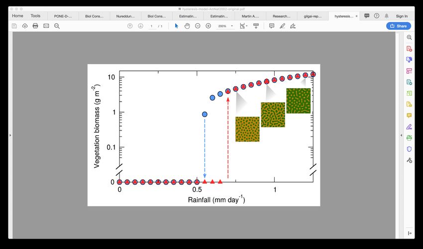
stochasticity (Weissmann et al., 2017), vegetation and soil type (Kéfi et al., 2007b), colonization rates
(Corrado et al., 2015), and intensity of external stresses, such as grazing (Kéfi et al., 2007a). Because
drylands cover ∼ 40% of Earth’s land surface and are home to ∼ 35% of the world population (Mortimore
et al., 2009), determining whether they will respond abruptly or gradually to aridification is critical both
from an ecosystem-management and socio-economic point of view.
    Active lines of theoretical research aiming to address this question have focused on understanding
how different components of the ecosystem may interact with each other to determine an ecosystem’s
response to aridification (Bonachela et al., 2015; Yizhaq and Bel, 2016), as well as on designing synthetic
feedbacks (in the form of artificial microbiomes) that could prevent ecosystems collapses or make such
transitions smoother (Villa Martín et al., 2015; Conde-Pueyo et al., 2020; Vidiella et al., 2020). The
question has also attracted considerable attention from empirical researchers (Maestre et al., 2016), and
recent evidence suggests that certain structural and functional ecosystem attributes respond abruptly
to aridity (Berdugo et al., 2020). Despite current efforts, whether desertification is more likely to occur
gradually or abruptly remains largely unknown.
    Here, we outline and rank strategies that will help answer this question. In section 2, we discuss
the ecological rationale behind existing models for vegetation self-organization. We review such models
in section 3 and summarize their opposing predictions about the ecosystem collapse in section 4. In
section 5, we describe possible manipulative experiments and empirical measures to select among the
previously scrutinized models. Finally, in section 6, we discuss different research lines that build on
current knowledge and discuss how to apply lessons learned from studying self-organized vegetation
patterns to other self-organizing systems.

2    Ecological rationale behind current models for vegetation spa-
     tial self-organization
The net biotic interaction between plants, i.e., the effect that plants have on each other’s survival, repro-
duction, and growth rate ultimately determines vegetation spatial patterns. Depending on the number of
individuals that form each patch, we can classify non-random vegetation spatial patterns into two fami-
lies: segregated and aggregated patterns (Fig. 2b). Segregated patterns emerge when competition is the
dominant net biotic interaction and surviving individuals avoid interacting with each other. In the long
term, vegetation arranges in a hexagonal lattice of patches with each individual representing one patch
(Pringle and Tarnita, 2017). Aggregated patterns, on the other hand, emerge when surviving plants form
vegetation patches with several individuals. Segregated patterns are very common in drylands and are
expected to emerge exclusively due to ecological interference or competition (Pringle and Tarnita, 2017).
Aggregated patterns, which are the focus of this study, are ecologically more intriguing because they
might result from a richer set of mechanisms (van de Koppel et al., 2008; Rietkerk and van de Koppel,
2008; Lee et al., 2021) and their ecological implications strongly depend on them (Fig. 2c, d). Moreover,
a direct evidence of which feedback type drives aggregated patterns of vegetation in drylands remains
elusive.
    Existing theories for vegetation self-organization hypothesize two alternative ways for the formation
of aggregated patterns: scale-dependent feedbacks (SDF) and purely competitive feedbacks (PCF). Both
are based on the biophysical effects of the plant canopy on the microclimate underneath and of the root
system on the soil conditions (Cabal et al., 2020b) (Fig. 2c), but they differ in how the net interaction
between plants changes with the inter-individual distance. Next, we will briefly review the mechanisms
that have been suggested to underpin each of these two feedbacks and the type of patterns they might
create.
    Scale-dependent feedbacks. Biotic facilitation is a very common interaction in semiarid and arid
ecosystems (Holmgren and Scheffer, 2010). The SDFs invoked to explain vegetation self-organization
are caused by the facilitative effects of plants nearby their stems, coupled with negative effects at longer
distances. Several ecological processes have been suggested to support these SDFs. One is the positive
effects of shade, which can overcome competition for light and the effects of root competition for water,
and lead to under-canopy facilitation (Valladares et al., 2016). In this context, focal plants have an overall
facilitative effect in the area of most intense shade at the center of the crown. This effect progressively
loses intensity with distance to the center of the crown and ultimately vanishes, leaving just simple below-
ground competition in areas farther from the plant. A complementary rationale is that plants modify
soil crust, structure, and porosity, and therefore enhance soil water infiltration (Eldridge et al., 2000;
Ludwig et al., 2004). Enhanced water infiltration has a direct positive effect close to the plant because

                                                      3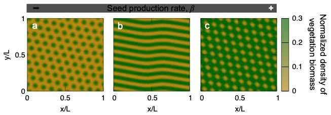
it increases soil water content but, as a by-product, it has negative consequences farther away from the
    plant’s insertion point because, by increasing local infiltration, plants also reduce the amount of water
    that can infiltrate further away in bare soil locations (Montaña, 1992; Bromley et al., 1997). The spatial
    heterogeneity in water availability due to plant-enhanced infiltration is higher in sloped landscapes where
    down-slope water runoff leads to the formation of banded vegetation patterns (Deblauwe et al., 2012;
    Valentin et al., 1999), but it is also significant in flat landscapes and might cause the of emergence gaps,
    labyrinths, and spots of vegetation (HilleRisLambers et al., 2001; Gilad et al., 2004; Okayasu and Aizawa,
    2001). (Fig. 2a).
Bare soil

                                                                       Crown range
            a    HUMID
                          b                          c                                                                Negative
                                                                                                                      feedback
                                                                                                                      Positive
                                                                                                                      feedback
                                                                                     Root system                      Adult individual
                                                                                       range                          crown
                                                                                                                      Multi-individual
                              Random (no pattern)                                                                     vegetation patch

                                                                                                   d
                                                           PURELY COMPETITIVE FEEDBACK (PCF)                        Gradual shifts

                                                      NI

                                                                                                   Veg. biomass
                                                         0
                              Segregated pattern

                                                                                                                           Rainfall

                                                           SCALE DEPENDENT FEEDBACK (SDF)                         Catastrophic shifts

                                                      NI

                                                                                                   Veg. biomass
                                                         0
                               Aggregated pattern
                  ARID
                                                                        Location                                           Rainfall

    Figure 2: Conceptual summary of existing theories for vegetation self-organization, their emergent patterns
    and the type of desertification processes they predict. a) Observed spatial patterns across a gradient of rainfall,
    with more humid ecosystems showing gaps and more arid, spots. b) Examples of spatial random, segregated,
    and aggregated patterns as defined in the main text. Aggregated patterns may result both from PCF and
    SDF, whereas segregated patterns emerge from PCF. c) Types of feedbacks invoked to explain the emergence of
    self-organized vegetation patterns and d) the different desertification transitions they predict.

        Purely competitive feedbacks. On the other hand, competition for resources is a ubiquitous interaction
    mechanism that affects the relation between any two plants that are located in sufficient proximity.
    Above ground, plants compete for light through their canopies; below ground, they compete for several
    soil resources, including water and nitrogen, through their roots (Craine and Dybzinski, 2013). If only
    competitive mechanisms occur, we should expect plants to have a negative effect on any other plant within
    their interaction range (Fig. 2c) and the intensity of this effect to peak at intermediate distances between
    vegetation patches(van de Koppel and Crain, 2006; Rietkerk and van de Koppel, 2008). Because finite-
    range competition is the only interaction required by PCF models to explain vegetation self-organization,
    PCF is the most parsimonious feedback type that generates vegetation patterns.

    3           Models for vegetation self-organization
    Mathematical frameworks to vegetation self-organized are grouped into two main categories: individual-
    based models (IBM) and partial differential equations models (PDEM). IBMs describe each plant as
    a discrete entity whose attributes change in time following a stochastic updating rule (DeAngelis and
    Yurek, 2016; Railsback and Grimm, 2019). PDEMs describe vegetation biomass and water concentration
    as continuous fields that change in space and time following a system of deterministic partial differential
    equations (Meron, 2015). IBM are the most convenient approach to study segregated patterns, where

                                                              4
single individuals are easy to identify and central to the formation of vegetation patches (Bolker and
Pacala, 1999; Iwasa, 2010; Wiegand and Moloney, 2013; Plank and Law, 2015). Conversely, PDEMs are
a better approximation to aggregated patterns because they focus on a continuous measure of vegetation
abundance and describe the dynamics of patches that can spread or shrink without any upper or lower
limit on their size. Natural multi-individual patches can change in size and shape depending on the
interaction among the individual plants within them, whereas the size of single-plant patches is subject
to stronger constraints (they usually grow, not shrink, and their maximum size is bounded by plant
physiology). Therefore, PDEMs represent a simplification of the biological reality that is more accurate
in aggregated than in segregated patterns. Because we are only considering aggregated patterns, we will
focus our review of the mathematical literature on PDEMs.

3.1     Reaction-diffusion SDF models
In 1952, Turing showed that differences in the diffusion coefficients of two reacting chemicals can lead to
the formation of stable spatial heterogeneities in their concentration (Turing, 1952). In Turing’s original
model, one of the chemicals acts as an activator and produces both the second chemical and more of
itself via an autocatalytic reaction. The second substance inhibits the production of the activator and
therefore balances its concentration (Fig. 3a). Spatial heterogeneities in the concentrations can form if
the inhibitor diffuses much faster than the activator, so that it inhibits the production of the activator at
a long range and confines the concentration of the activator locally (Fig. 3b). This activation-inhibition
principle thus relies on a SDF to produce patterns: positive feedbacks (autocatalysis) dominate on short
scales and negative, inhibitory feedbacks dominate on larger scales. In the context of vegetation pattern
formation, plant biomass acts as the self-replicating activator. Water is a limiting resource and thus
water scarcity is an inhibitor of vegetation growth (Rietkerk and van de Koppel, 2008; Meron, 2012).

              a                   kaa                   b                        Activator        Inhibitor

                  Da            Activator
                                                             Concentration

                                                                                                          Time
                          kai               kia

             Di                 Inhibitor

                                                                             Spatial coordinate

Figure 3: a) Schematic of the Turing activation-inhibition principle. The activator, with diffusion coefficient
Da , produces the inhibitor at rate kai as well as more of itself at rate kaa through an autocatalytic reaction. The
inhibitor degrades the activator at rate kia and diffuses at rate Di > Da . b) Schematic of the pattern-forming
process in a one-dimensional system.

3.1.1   Two-equation water-vegetation dynamics: the generalized Klausmeier model
Initially formulated to describe the formation of stripes of vegetation in sloping landscapes (Fig. 1d),
subsequent studies have generalized the Klausmeier model to flat surfaces (Kealy and Wollkind, 2011;
Bastiaansen et al., 2018; Eigentler and Sherratt, 2020). Mathematically, the generalized version of the
Klausmeier model is given by the following equations:

                       ∂w(r, t)
                                   = R − l w(r, t) − a g (w) f (v) v(r, t) + Dw ∇2 w(r, t),                      (1)
                         ∂t
                       ∂v(r, t)
                                   = a q g (w) f (v) v(r, t) − m v(r, t) + Dv ∇2 v(r, t),                        (2)
                         ∂t

                                                         5
where w(r, t) and v(r, t) represent water concentration and density of vegetation biomass at location r
and time t, respectively. In Eq. (1), water is continuously supplied at a precipitation rate R, and its
concentration decreases due to physical losses such as evaporation, occurring at rate l (second term),
and local uptake by plants (third term). In the latter, a is the plant absorption rate, g(w) describes the
dependence of vegetation growth on water availability, and f (v) is an increasing function of vegetation
density that represents the positive effect that the presence of plants has on water infiltration. Finally,
water diffuses with a diffusion coefficient Dw . Similarly, Eq. (2) accounts for vegetation growth due to
water uptake (first term), plant mortality at rate m (second term), and plant dispersal (last term). In
the plant growth term, the parameter q represents the yield of plant biomass per unit of consumed
water; although the original model assumed for mathematical simplicity linear absorption rate and plant
response to water (g(w) = w(r, t) and f (v) = v(r, t)), other biologically-plausible choices can account
for processes such as saturation in plant growth due to intraspecific competition (Eigentler, 2020).
The generalized Klausmeier model with linear absorption rate and plant responses to water has
three spatially-uniform equilibria obtained from the fixed points of Eqs. (1)-(2): an unvegetated state
(v ∗ = 0, w∗ = R/l), stable for any value of the rainfall parameter R; and two states in which vegetation
and water coexist at different non-zero values. Only the vegetated state with higher vegetation biomass
is stable against non-spatial perturbations, and only for a certain range of values of R. The latter suffices
to guarantee bistability, that is, the presence of alternative stable states (vegetated vs unvegetated), and
hysteresis. For spatial perturbations, however, the stable vegetated state becomes unstable within a
range of R, and the system develops spatial patterns.
3.1.2 Three-equation water-vegetation dynamics: the Rietkerk model
The Rietkerk model extends the generalized Klausmeier model by splitting Eq. (1) into two equations
(one for surface water, and another one for soil water) and including a term that represents water
infiltration. Moreover, the functions that represent water uptake and infiltration are nonlinear, which
introduces additional feedbacks between vegetation, soil water, and surface water. The model equations
are as follows:
∂u(r, t) v(r, t) + k2 w0
= R−α u(r, t) + Du ∇2 u(r, t) (3)
∂t v(r, t) + k2
∂w(r, t) v(r, t) + k2 w0 v(r, t) w(r, t)
= α u(r, t) − gm − δw w(r, t) + Dw ∇2 w(r, t) (4)
∂t v(r, t) + k2 k1 + w(r, t)
∂v(r, t) v(r, t) w(r, t)
= c gm − δv v(r, t) + Dv ∇2 v(r, t) (5)
∂t k1 + w(r, t)
where u(r, t), w(r, t), and v(r, t) are the density of surface water, soil water, and vegetation, respectively.
In Eq. (3), R is the mean annual rainfall, providing a constant supply of water to the system; the second
term accounts for infiltration; and the diffusion term accounts for the lateral circulation of water on
the surface. In Eq. (4), the first term represents the infiltration of surface water into the soil, which is
enhanced by the presence of plants; the second term represents water uptake; the third one accounts for
physical losses of soil water, such as evaporation; and the diffusion term describes the lateral circulation
of underground water. Finally, the first term in Eq. (5) represents vegetation growth due to the uptake of
soil water, which is a function that saturates for high water concentrations; the second term accounts for
biomass loss at constant rate due to natural death or external hazards; and the diffusion term accounts
for plant dispersal. The meaning of each parameter in the equations, together with the values used in
Rietkerk et al. (2002) for their numerical analysis, are provided in Table 1.
In the spatially uniform case, this model allows for two different steady states: a vegetated state
in which vegetation, soil water, and surface water coexist at non-zero values; and an unvegetated (i.e.,
desert) state in which only soil water and surface water are non-zero. Considering the parameterization
in Table 1, the stability of each of these states switches at R = 1. For R < 1, only the unvegetated
equilibrium is stable against non-spatial perturbations, whereas for R > 1 the vegetated equilibrium
becomes stable and the desert state, unstable. When allowing for spatial perturbations, numerical
simulations using the parameterization in Table 1 show the existence of spatial patterns within the
interval 0.7 . R . 1.3, which is in agreement with analytical approximations (Gowda et al., 2016).
Within this range of mean annual rainfall, the patterns sequentially transition from gaps to labyrinths
to spots with increasing aridity. For R ≈ 0.7, the system transitions abruptly from the spotted pattern
to the desert state.
6Parameter Symbol Value
c Water-biomass conversion factor 10 (g mm−1 m−2 )
α Maximum infiltration rate 0.2 (day−1 )
gm Maximum uptake rate 0.05 (mm g−1 m−2 day−1 )
w0 Water infiltration in the absence of plants 0.2 (-)
k1 Water uptake half-saturation constant 5 (mm)
k2 Saturation constant of water infiltration 5 (g m−2 )
δw Soil water loss rate 0.2 (day−1 )
δv Plant mortality 0.25 (day−1 )
Dw Soil water lateral diffusion 0.1 (m2 day−1 )
Dv Vegetation dispersal 0.1 (m2 day−1 )
Du Surface water lateral diffusion 100 (m2 day−1 )
Table 1: Typical parameterization of the Rietkerk model (Rietkerk et al., 2002).
The Rietkerk model assumes constant rainfall, homogeneous soil properties, and only local and short-
range processes. Therefore, all the parameters are constant in space and time, and patterns emerge from
SDFs between vegetation biomass and water availability alone. This simplification is, however, not valid
for most ecosystems. Arid and semi-arid regions feature seasonal variability in rainfall (Salem et al.,
1989). Kletter et al. (2009) showed that, depending on the functional dependence between water uptake
and soil moisture, stochastic rainfall might increase the amount of vegetation biomass in the ecosystem
compared to a constant rainfall scenario. Moreover, the properties of the soil often change in space.
A widespread cause of this heterogeneity is soil-dwelling macrofauna, such as ants, earthworms, and
termites (Pringle and Tarnita, 2017). Bonachela et al. (2015) found that heterogeneity in substrate
properties induced by soil-dwelling macrofauna, and modeled by space-dependent parameters, might
interact with SDFs between water and vegetation and introduce new characteristic spatial scales in the
pattern. Finally, researchers have also extended the Rietkerk model to account for long-range, nonlocal
processes. For example, Gilad et al. (2004) introduced a nonlocal mechanism in the interaction between
vegetation biomass and soil water of Eqs. (4)-(5) to model the water conduction of lateral roots towards
the plant canopy. As explained in the next section, although this model accounts for nonlocal processes,
it is conceptually very different from kernel-based models.
3.2 Kernel-based SDF models
Kernel-based models are those in which all the feedbacks that control the interaction between plants
are encapsulated in a single nonlocal net interaction between plants. The nonlocality in the net plant
interaction accounts for the fact that individual (or patches of) plants can interact with each other within
a finite neighborhood. Therefore, the vegetation dynamics at any point of the space is coupled to the
density of vegetation at locations within the interaction range. Because all feedbacks are collapsed into
a net interaction between plants, kernel-based models do not describe the dynamics of any type of water
and use a single partial integro-differential equation for the spatiotemporal dynamics of the vegetation.
The kernel is often defined as the addition of two Gaussian functions with different widths, with the wider
function taking negative values to account for the longer range of competitive interactions (D’Odorico
et al., 2006) (central panels of Fig. 2).
3.2.1 Models with additive nonlocal interactions
In the simplest kernel-based SDF models, the spatial coupling is introduced linearly in the equation for
the local dynamics (D’Odorico et al., 2006),
Z
∂v(r, t)
= h (v) + dr 0 G (r 0 ; r) [v (r 0 , t) − v0 ] . (6)
∂t
The first term describes the local dynamics of the vegetation, i.e., temporal changes in vegetation density
at a location r due to processes in which neighboring vegetation does not play any role. The integral
term describes any spatial coupling, i.e., changes in vegetation density at r due to vegetation density
at neighbor locations r’. Assuming spatial isotropy, the kernel function G(r, r 0 ) decays radially with
the distance from the focal location, |r 0 − r|, so G (r 0 , r) = G(|r 0 − r|). Therefore, the dynamics of the
vegetation density is governed by two main contributions: first, if the spatial coupling is neglected, the
7vegetation density increases or decreases locally depending on the sign of h(v) until reaching a uniform
steady state v0 , solution of h(v0 ) = 0; second, the spatial coupling enhances or diminishes vegetation
growth depending on the sign of the kernel function (i.e., whether the spatial interactions affect growth
positively or negatively) and the difference between the local vegetation density and the uniform steady
state v0 .
Assuming kernels that are positive close to the focal location and negative far from it (a la SDF),
local perturbations in the vegetation density around v0 are locally enhanced if they are larger than
v0 and attenuated otherwise. As a result, the integral term destabilizes the homogeneous state when
perturbed, and spatial patterns arise in the system. Long-range growth-inhibition interactions, together
with nonlinear terms in the local-growth function h(v), avoid the unbounded growth of perturbations
and stabilize the pattern. However, although this mechanism imposes an upper bound to vegetation
density, nothing prevents v from taking unrealistic, negative values. To avoid this issue, the model must
include an artificial bound at v = 0 such that vegetation density is reset to zero whenever it becomes
negative.
3.2.2 Models with multiplicative nonlocal interactions
A less artificial way to ensure that vegetation density remain always positive is to modulate the spatial
coupling with nonlinear terms. For example, the pioneering model developed by Lefever and Lejeune
(1997) consists of a modified logistic equation in which each of the terms includes an integral term to
encode long-range spatial interactions,
∂v(r, t) (ω2 ∗ v) (r, t)
= β (ω1 ∗ v) (r, t) 1 − − η (ω3 ∗ v) (r, t) (7)
∂t K
where β is the rate at which seeds are produced (a proxy for the number of seeds produced by each plant)
and η is the rate at which vegetation biomass is lost due to spontaneous death and external hazards
such as grazing, fires, or anthropogenic factors (last term). The model assumes spatial isotropy, and the
symbol ∗ indicates a linear convolution operation:
Z
(ωi ∗ v) (r, t) = dr 0 ωi (r − r 0 ; `i )v(r 0 , t) i = 1, 2, 3 (8)
in which each ωi is a weighting function with a characteristic spatial scale `i that defines the size of
the neighborhood contributing to the focal process. For instance, ω1 (r − r 0 ; `1 ) defines the size of
the neighborhood that contributes to the growth of vegetation biomass at r. Similarly, `2 defines the
scale over which plants inhibit the growth of their neighbors, and `3 the scale over which vegetation
density influences the spontaneous death rate of vegetation at the focal location. Because the sign of
the interaction is explicit in each term of Eq. (7), the convolutions only represent weighted averages of
vegetation biomass and the weighting functions are always positive. In addition, because Lefever and
Lejeune (1997) set the scale of the inhibitory interactions larger than the scale of the positive interactions
(`2 > `1 ), the model includes a SDF with short-range facilitation and long-range competition.
Expanding upon this work, several other models have introduced non-linear spatial couplings via
integral terms (Fernandez-Oto et al., 2014; Escaff et al., 2015; Berríos-Caro et al., 2020), and others have
expanded the integral terms and studied the formation of localized structures of vegetation (Parra-Rivas
and Fernandez-Oto, 2020).
3.3 Kernel-based PCF models.
In previous sections, we invoked the existence of SDFs in the interactions among plants to explain the
emergence of self-organized spatial patterns of vegetation. Both theoretical and empirical studies, how-
ever, have highlighted the importance of long-range negative feedbacks on pattern formation, suggesting
that short-range positive feedbacks might be secondary actors that sharpen the boundaries of clusters
rather than being key for the instabilities that lead to the patterns (van de Koppel and Crain, 2006;
Rietkerk and van de Koppel, 2008; van de Koppel et al., 2008). Following these arguments, Martínez-
García et al. (2013a), (2014) proposed a family of purely competitive models with the goal of identifying
the smallest set of mechanisms needed for self-organized vegetation patterns to form.
The simplest PCF models consider additive nonlocal interactions (Martínez-García et al., 2014).
Alternatively, nonlocal interactions can be represented through nonlinear functions modulating either
the growth or the death terms. In both cases, the models develop the full sequence of patterns (gaps,
8labyrinths, and spots). The model proposed in Martínez-García et al. (2013a) introduces competition
through the growth term:
∂v(r, t) v(r, t)
v , δ) β v(r, t) 1 −
= PE (e − η v(r, t), (9)
∂t K
where β and K are the seed production rate and the local carrying capacity, respectively. δ is the
competition-strength parameter, and ve (r, t) is the average density of vegetation around the focal position
r: Z
ve (r, t) = dr 0 G (|r 0 − r|) v (r 0 , t) . (10)
where the kernel function G, assumes spatial isotropy and weighs how vegetation at a location r 0 con-
tributes to the average vegetation density around r, and is necessarily defined positive. Because it is a
weighting function, G plays the same role and has the same properties described for the ωi functions in
section 3.2. The model further assumes that vegetation losses occur at constant rate η and vegetation
grows through a three-step sequence of seed production, local dispersal, and establishment (Calabrese
et al., 2010), represented by the three factors that contribute to the first term in Eq. (9). First, plants
produce seeds at a constant rate β, which leads to the a growth term βv(r, t). Second, seeds disperse
locally and compete for space which defines a local carrying capacity K. Third, plants compete for
resources with other plants, which is modeled using a plant establishment probability, PE . Because the
only long-range interaction in the model is root-mediated interference, and competition for resources is
more intense in more crowded environments, PE is a monotonically decreasing function of the nonlocal
vegetation density ṽ(r, t) defined in Eq. (10). Moreover, PE also depends on the competition-strength
parameter, δ, representing resource limitation. In the limit δ = 0, resources are abundant, competition
is weak, and PE = 1. Conversely, in the limit δ → ∞, resources are very scarce, competition is very
strong, and PE → 0.
In PCF models, spatial patterns form solely due to the long-range competition. If patches are far
enough from each other, individuals attempting to establish in between patches compete with vegetation
from more than one adjacent patch, whereas individuals within a patch only interact with plants in that
same patch. As a result, competition is more intense in the regions between patches than inside each
patch, which stabilizes an aggregated pattern of vegetation (Fig. 4) whose shape (gaps, labyrinths or
spots) will depend on the model parameterization. This same mechanism has been suggested to drive
the formation of clusters of competing species in the niche space (Scheffer and van Nes, 2006; Pigolotti
et al., 2007; Hernández-García et al., 2009; Fort et al., 2009; Leimar et al., 2013) and the aggregation
of individuals in models of interacting particles with density-dependent reproduction rates (Hernández-
García and López, 2004).
a b c
Figure 4: In PCF models, patchy distributions of vegetation in which the distance between patches is between
one and two times the range of the nonlocal interactions are stable. Individuals within each patch only compete
with the individuals in that patch (a,b), whereas individuals in between patches compete with individuals from
both patches (c). Color code: green trees are focal individuals, and dashed circles limit the range of interaction
of the focal individual. Dark grey is used for individuals that interact with the focal one, whereas light gray
indicates individuals that are out of the range of interaction of the focal individual.
94 Self-organized patterns as indicators of ecological transitions
Models using different forms for the net biotic interaction between neighbor patches (SDF vs PCF) have
successfully reproduced qualitatively the spatial patterns of vegetation observed in water-limited ecosys-
tems (Deblauwe et al., 2011). All these different models also predict that the spotted pattern precedes
a transition to an unvegetated state, which positions it as an early-warning indicator of desertification
transitions (Scheffer et al., 2009; Dakos et al., 2011). Despite the similar prediction, models with different
underlying mechanisms for the formation of these patterns result in different desertification processes.
The Rietkerk model from section 3.1.2, for example, predicts that self-organized ecosystems eventually
collapse following an abrupt transition that includes a hysteresis loop (Fig. 5a). Abrupt transitions such
as this one are typical of bistable systems in which the stationary state depends on the environmental
and the initial conditions. Bistability is a persistent feature of models for vegetation pattern formation,
sometimes occurring also in transitions between patterned states (von Hardenberg et al., 2001). It also
denotes the existence of thresholds in the system that trigger sudden, abrupt responses in its dynamics.
These thresholds are often created by positive feedbacks or quorum-regulated behaviors, as is the case in
populations subject to strong Allee effects (Courchamp et al., 1999). In the Rietkerk model, as rainfall
decreases, the spatial distribution of vegetation moves through the gapped-labyrinthine-spotted sequence
of patterns (Fig. 5a). However, when the rainfall crosses a threshold value the system responds abruptly,
and all vegetation dies. Setting up the simulations as indicated in Rietkerk et al. (2002) and using the
parameterization of Table 1, this threshold is located at R ≈ 0.55 mm day−1 . Once the system reaches
this unvegetated state, increasing water availability does not allow vegetation recovery until R ≈ 0.70
mm day−1 , which results in a hysteresis loop and a region of bistability (R ∈ [0.55, 0.70] in Fig. 5a).
Bistability and hysteresis loops make abrupt, sudden transitions like this one extremely hard to revert.
Hence, anticipating such abrupt transitions is crucial from a conservation and ecosystem-management
point of view (Scheffer et al., 2009; Dakos et al., 2011).
Extended versions of the Rietkerk model have suggested that the interaction between vegetation
and other biotic components of the ecosystem may change the transition to the unvegetated state.
Specifically, Bonachela et al. (2015) suggested that soil-dwelling termites, in establishing their nests
(mounds), engineer the chemical and physical properties of the soil in a way that turns the abrupt
desertification into a two-step process (Fig. 5b). At a certain precipitation level (R ≈ 0.75 mm day−1
using the parameterization in Table 1 and the same initial condition used for the original Rietkerk model),
vegetation dies in most of the landscape (T1 in Fig. 5b) but persists on the mounds due to improved
properties for plant growth created by the termites. On-mound vegetation survives even if precipitation
continues to decline, and is finally lost at a rainfall threshold R ≈ 0.35 mm day−1 (T2 in Fig. 5b).
As a consequence of the two-step transition, the ecosystem collapse is easier to prevent because a bare
soil matrix with vegetation only on mounds serves as an early-warning signal of desertification, and it is
easier to revert since termite-induced heterogeneity breaks the large hysteresis loop of the original model
into two smaller ones (compare the hysteresis loops in Figs. 5a and 5b).
On the other hand, the PCF model in Martínez-García et al. (2013a), (2013b) discussed in section
3.3 predicts a smooth desertification in which vegetation biomass decreases continuously in response to
decreasing seed production rate (a proxy for worsening environmental conditions). It is important to say
that considering local vegetation dispersal, and thus not introducing a diffusive term in model Eq. (9),
is also one of the assumptions leading to this smooth transition. According to this model, the spotted
pattern would persist as precipitation declines, with vegetation biomass decreasing until it eventually
disappears (Fig. 5c). As opposed to the catastrophic shift described for the Rietkerk model, smooth
transitions such as the one depicted by this model do not show bistability and do not feature hysteresis
loops. This difference has important socio-ecological implications, because it enables easier and more
affordable management strategies to restore the ecosystem after the collapse (Villa Martín et al., 2015).
Moreover, continuous transitions are also more predictable because the density of vegetation is univocally
determined by the control parameter (seed production rate β in Fig. 5c).
10101 a
Vegetation biomass (g m-2)
100
10-1
Increasing R
Decreasing R
10-2
0.25 0.75 1.25
Rainfall (mm day ) -1
0.3
101
b c
Normalized vegetation density
Vegetation biomass (g m-2)
0.2
100 (T1)
10-1 0.1
(T2)
10-2 0
0.25 0.75 1.25 0 5 10 15 20
Rainfall (mm day-1) Seed production rate, β
Figure 5: Although different models for vegetation pattern formation may recover the same sequence of gapped-
labyrinthine-spotted patterns from different mechanism, the type of desertification transition that follows the
spotted pattern strongly depends on the model ingredients. a) Abrupt desertification as predicted by the Rietkerk
model (Rietkerk et al., 2002). b) Two-step desertification process as predicted in Bonachela et al. (2015) when
soil-dwelling insects are added to the Rietkerk model. c) Progressive desertification as predicted by the PCF
model introduced in Martínez-García et al. (2013a). For each panel, numerical simulations were conducted using
the same setup described in the original publications.
In the three scenarios discussed above, patterns have tremendous potential for ecosystem management
as an inexpensive and reliable early indicator of ecological transitions (Scheffer et al., 2009; Dakos et al.,
2011). However, the different predictions that models make about the transition highlights the need
for tailored models that not only reproduce the observed patterns but do so through the mechanisms
relevant to the focal system. We have shown that widespread spotted patterns can form in models
accounting for very different mechanisms (Fig. 5). Because ecosystems are highly complex, it is very
likely that spotted patterns observed in different regions emerge from very different mechanisms (or
combinations of them) and thus anticipate very different transitions (Kéfi et al., 2007a,b; Corrado et al.,
2015; Weissmann et al., 2017). Therefore, a reliable use of spotted patterns as early warning indicators
of ecosystem collapse requires (i) mechanistic models that are parameterized and validated by empirical
observations of both mechanisms and patterns; (ii) quantitative analyses of field observations; and (iii)
manipulative experiments.
5 Testing models for vegetation self-organization in the field
As depicted through this review, the study of self-organized vegetation patterns has been mostly theo-
retical and empirical evidences of the self-organization hypotheses explaining the formation of vegetation
spatial patterns are much less widespread. In this section, we explore the possible empirical approaches to
understanding the mechanisms responsible for the formation and persistence of self-organized aggregated
patterns and propose a two-step protocol to this end.
At least three possible approaches exist to study existing self-organization hypotheses for pattern
formation in natural systems. First, the observation and measurement of the spatial structure of pat-
11terns from aerial and satellite photography (the observational approach). Second, the assessment of the
net interactions among plants or plant patches as a function of the distance between them (the net-
interaction approach). Third, the investigation of the specific mechanisms underpinning that interaction
(the selective mechanistic approach). The observational approach has been relatively common, and is
the one that has motivated the development of most existing models (Borgogno et al., 2009; Wu et al.,
2000). Nevertheless, without a more detailed understanding of the focal systems, one cannot discard
whether agreement between model predictions and natural observations is coincidental. The mechanis-
tic approach has been relatively common. Some studies have investigated selectively the mechanisms
potentially leading to pattern formation in tiger bush banded vegetation in Niger (Valentin and Poesen,
1999), vegetation rings in Israel (Sheffer et al., 2011; Yizhaq et al., 2019), or fairy circles in Namibia
(Ravi et al., 2017) and Australia (Getzin et al., 2021). To our knowledge, the net-interaction approach is
conspicuous by being absent, and researchers have scarcely measured directly the net interaction among
plants or vegetation patches and its variation with the inter-plant distance in patterned ecosystems.
Because we are discussing here aggregated patterns, a first step in such approach is to confirm that
vegetation patches are formed by several aggregated individuals. In the case of segregated patterns, we
recommend the use of point pattern analysis under the hypothesis of the dominance of competition forces
(Franklin, 2010). Following this preliminary test, we propose a two-step protocol to conduct future field
reseearch on the emergence and maintenance of vegetation spatial patterns.
First step: phenomenological investigation of the net interaction among plants within the vegetated
patch and in bare soil. This first step is needed because a myriad of alternative mechanisms can explain
the formation of spatial patterns, some of them well aligned with the idea of vegetation self-organization
and others dependent on external biological or geological factors. For example, in the case of fairy
circles researchers have explored the role of higher evaporation (Vlieghe and Picker, 2019) and increased
termite activity (Juergens, 2013) within the circles; spatial heterogeneity in hydrological processes, such
as increased infiltration in the circles of bare soil (Ravi et al., 2017) or increased water runoff in the
circles and in the matrix (Getzin et al., 2021); and the geological emanation of toxic gases (Naudé et al.,
2011) and the presence of allelochemical substances (Meyer et al., 2020) in the circles. By using a
phenomenological approach as a first step, researchers can discard many of these potential mechanisms,
directing their efforts towards more specific hypotheses in a second step. For this first step, a simple
experimental setup, based on mainstream methods to measure plant biotic interaction would reveal
whether PCF, SDF, or none of them are responsible for the emergent pattern (Armas et al., 2004).
Our proposed experiment would compare a fitness proxy (e.g., growth, survival) of experimental plants
planted in the system under study, where we observe a regular vegetation pattern and we assume that
the vegetation vegetation dynamics has reached a stationary state for the location-specific environmental
conditions. Each experimental block would consist of a plant growing under-canopy (Fig. 6a), a plant
growing in bare soil (i.e., between two vegetation patches) (Fig. 6b), and a control plant growing in the
same ecosystem but artificially isolated from the interaction with pattern-forming individuals (Fig. 6c).
To isolate control plants from canopy interaction they need to be planted in bare soil areas. To isolate
them from below-ground competition, one can excavate narrow, deep trenches in which a root barrier
can be inserted (Morgenroth, 2008). To isolate them from the competition for runoff water with the
vegetation patches, root barriers should protrude from the soil a few centimeters, preventing precipitation
water to leave the area and runoff water to enter. Comparing the fitness proxy of the control plant with
that of plants growing in vegetation patches or bare soil reveals the sign and strength of the net biotic
interaction. By replicating this experimental block, we can statistically determine whether the pattern
formation results from a SDF, a PCF, or whether it involves a different process. The SDF hypothesis
would be validated if a predominantly positive net interaction is observed under the canopy, and a
negative interaction is observed in bare soils. Conversely, the PCF would be validated if we observe a
negative net interaction in bare soils and under canopy (see Table 2). Any other outcome in the spatial
distribution of the sign of the net interaction between plants would suggest that other mechanisms are at
play, which could include the action of different ecosystem components, such as soil-dwelling macrofauna
(Tarnita et al., 2017), or abiotic factors, such as micro-topology.
Second step: direct measurement of the biophysical processes responsible for the pattern. After con-
firming the PCF, the SDF, finding an alternative spatial distribution of plant interactions or rejecting
the self-organizing hypothesis, a second experimental step would test specific biophysical mechanisms
responsible for the measured interaction and driving the spatial pattern. For example, PCF models
hypothesize that spatial patterns are driven by long-range below-ground competition for a limiting re-
source through the formation of exclusion regions. As discussed in section 3.3, these exclusion regions
are territories between patches of vegetation in which the intensity of competition is higher than within
12Canopy range
Bare soil Bare soil
(c) (a) (b)
Root
barrier
Figure 6: Schematic representation of a simple experimental setup to test in the field whether the mechanism of
spatial patterning is a purely competitive feedback (PCF) or a classic scale-dependent feedback (SDF). Plant (a)
is an experimental plant growing under-canopy, (b) is growing in bare soil, and (c) is a control plant growing in
artificial conditions, free from the biotic interaction using root barriers in bare soil areas of the same environment.
Under canopy vs control Bare soil vs control Outcome
0/− − − Purely competitive feedback
+ − Scale-dependent feedback
Table 2: Testing the PCF versus SDF hypotheses in the experimental setup introduced in Fig. 6. Double signs
indicate stronger intensity. Indexes to calculate the sign of the net interaction can be taken from Armas et al.
(2004).
the patch (van de Koppel and Crain, 2006), possibly because they present a higher density of roots
(Fig. 4) (Martínez-García et al., 2013a, 2014). To test for the existence of exclusion regions and confirm
whether below-ground competition is driving the spatial pattern, researchers can measure the changes
in root density using coring devices (Cabal et al., 2021) across soil transects going from the center of a
vegetated patch to the center of a bare soil patch. Field tests and manipulative experiments to confirm
that SDFs are responsible for vegetation patterns are not easy to perform but researchers can do a hand-
ful of analyses. For example, ecohydrological SDF models assume that water infiltration is significantly
faster in vegetation patches than in bare soil areas (Rietkerk et al., 2002). Many empirical researchers
have tested this assumption in patterned vegetation using mini disk infiltrometers to quantify unsatu-
rated hydraulic conductivity, dual head infiltrometers to measure saturated hydraulic conductivity, or
buried moisture sensors connected to data loggers to record volumetric soil moisture content (Yizhaq
et al., 2019; Ravi et al., 2017; Getzin et al., 2021; Cramer and Barger, 2013). The measures should show
higher infiltration rates and moisture under vegetated patches than in bare soil. Note, however, that
infiltration rates might be very hard to measure due to small-scale soil heterogeneities. Ecohydrological
models make other assumptions that are less often considered in the field. For instance, they assume that
the lateral transport of water is several orders of magnitude larger than vegetation diffusion (i.e., patch
growth speed), which might be true or not depending on soil properties. To test these assumptions, field
researchers need to measure the intensity of the water runoff and compare it to a measure of the lateral
growth rate of vegetation patches. Water runoff is very challenging to measure directly, but estimates
can be calculated using the infiltration rates obtained with infiltrometers (Cook, 1946). The lateral
growth rate of vegetation patches can be estimated based on drone or satellite images repeated over
time (Trichon et al., 2018). Combining measures of both water runoff and expansion rates of vegetation
patches, one can estimate approximated values for the relative ratio of the two metrics.
136 Conclusions and future lines of research
As our ability to obtain and analyze large, high-resolution images of the Earth’s surface increases, more
examples of self-organized vegetation patterns are found in water-limited ecosystems. Here, we have
reviewed different modeling approaches employed to understand the mechanistic causes and the predicted
consequences of those patterns. We have discussed how different models, relying on different mechanisms,
can successfully reproduce the patterns observed in natural systems and that, however, each of these
models predicts very different ecosystem-level consequences of the emergent pattern. This discrepancy
limits the utility of the patterns as applied ecological tools in the absence of explicit knowledge of
underlying mechanisms. To solve this issue, we claim that models need to move from their current
phenomenological formulation towards a more system-specific and mechanistic one. This new approach
must necessarily focus on isolating the system-specific, key feedbacks for vegetation self-organization.
We identify two main directions for future research to develop this new approach to vegetation pattern
formation.
First, biologically-grounded studies should aim to combine system-specific models with empirical
measures of vegetation-mediated feedbacks. Existing models for vegetation self-organization are mostly
phenomenological and are only validated qualitatively via the visual comparison of simulated and ob-
served (macroscopic) patterns. Experimental measures of the (microscopic) processes and feedbacks
central to most models of vegetation pattern formation are hard to obtain, leading to arbitrary (free) pa-
rameter values and response functions. For example, very few models incorporate empirically-validated
values of water diffusion and plant dispersal rates, despite the crucial role of these parameters in the
emergence of patterns. Instead, these models fine-tune such values to obtain patterns similar in, for
example, their wavelength, to the natural pattern. Similarly, we are only beginning to understand how
plants rearrange their root system in the presence of competing individuals (Cabal et al., 2020a), and
hence kernel-based models still do not incorporate realistic functional forms for the kernels. Instead, these
models use phenomenological functions to test potential mechanisms for pattern formation by qualita-
tively comparing model output and target pattern, thus limiting the potential of the models to make
quantitative predictions. To establish a dialogue between experiments and theory, models should develop
from a microscopic description of the system (DeAngelis and Yurek, 2016; Railsback and Grimm, 2019).
This approach allows for a more realistic and accurate description of the plant-to-plant and plant-water
interactions as well as for a better reconciliation between model parameters and system-specific empirical
measures. Hopefully it will also allow researchers to unify existing theoretical approaches to vegetation
pattern formation (Martínez-García et al., 2014). Subsequently, existing tools from mathematics, sta-
tistical physics, and/or computer science can be used to reach a macroscopic PDEM that captures the
key ingredients of the microscopic dynamics. Statistical physics, which was conceived to describe how
observed macroscopic properties of physical systems emerge from the underlying microscopic processes,
provides a compelling and well-developed framework to make such a micro-macro connection.
Second, recent developments in remotely sensed imagery have enabled the measurement of an ecosys-
tem’s state indicators, which will allow researchers to compare observed and simulated patterns quanti-
tatively (Bastiaansen et al., 2018). On the one hand, using existing databases of ecosystem responses to
aridity (Berdugo et al., 2020) and satellite imagery of vegetation coverage (Deblauwe et al., 2011), re-
searchers could conduct a model selection analysis and classify existing models from more to less realistic
depending on whether (and how many) features of the focal ecosystem the model manages to reproduce
in the correct environmental conditions. For example, models could be classified depending on whether,
after proper parameterization, they can predict ecosystem responses such as transitions between pattern
types at the correct aridity thresholds. To elaborate this model classification, the use of Fourier analysis
for identifying regularity in natural patterns, geostatistics for quantifying spatial correlations, and time
series analysis for tracking changes in the ecosystem properties through time will be essential.
Beyond water-limited ecosystems, SDFs have been invoked to explain spatial pattern formation in
mussel beds (Rietkerk and van de Koppel, 2008), freshwater and salt marshes (van de Koppel et al., 2005;
Van Wesenbeeck et al., 2008; Zhao et al., 2021), and seagrasses (van der Heide et al., 2011; Ruiz-Reynés
et al., 2017). Conversely, nonlocal competition drives the emergence of aggregated patterns in freshwater
marshes (van de Koppel et al., 2008) and in theoretical models of population dynamics (Fuentes et al.,
2003; Dornelas et al., 2019; Maruvka and Shnerb, 2006; Da Cunha et al., 2011; Clerc et al., 2005;
Maciel and Martinez-Garcia, 2020). Understanding the conditions in which negative feedbacks dominate
over positive feedbacks, finding the key features that distinguish the patterns caused by these different
feedbacks, and contrasting their divergent ecological consequences constitutes an exciting venue for future
research that has just started to develop (Lee et al., 2021).
14You can also read