A simulation-experiment-based assessment of retrievals of above-cloud temperature and water vapor using a hyperspectral infrared sounder - Recent
←
→
Page content transcription
If your browser does not render page correctly, please read the page content below
Atmos. Meas. Tech., 14, 5717–5734, 2021
https://doi.org/10.5194/amt-14-5717-2021
© Author(s) 2021. This work is distributed under
the Creative Commons Attribution 4.0 License.

A simulation-experiment-based assessment of retrievals of
above-cloud temperature and water vapor using a
hyperspectral infrared sounder
Jing Feng1 , Yi Huang1 , and Zhipeng Qu1,2
1 Department   of Atmospheric and Oceanic Sciences, McGill University, Montreal, Quebec, Canada
2 Observations-Based  Research Section, Environment and Climate Change Canada, Toronto, Ontario, Canada

Correspondence: Jing Feng (jing.feng3@mail.mcgill.ca)

Received: 4 January 2021 – Discussion started: 16 March 2021
Revised: 14 July 2021 – Accepted: 15 July 2021 – Published: 20 August 2021

Abstract. Measuring atmospheric conditions above convec-         tion of the ice water content and effective radius compared to
tive storms using spaceborne instruments is challenging. The     prior knowledge based on retrievals from active sensors. Our
operational retrieval framework of current hyperspectral in-     results suggest that existing infrared hyperspectral sounders
frared sounders adopts a cloud-clearing scheme that is un-       can detect the spatial distributions of temperature and humid-
reliable in overcast conditions. To overcome this issue, pre-    ity anomalies above convective storms.
vious studies have developed an optimal estimation method
that retrieves the temperature and humidity above high thick
clouds by assuming a slab of cloud. In this study, we find
that variations in the effective radius and density of cloud     1   Introduction
ice near the tops of convective clouds lead to non-negligible
spectral uncertainties in simulated infrared radiance spec-      Water vapor in the upper troposphere and lower stratosphere
tra. These uncertainties cannot be fully eliminated by the       (UTLS) plays an essential role in the Earth’s climate sys-
slab-cloud assumption. To address this problem, a syner-         tem due to its important radiative effects (Huang et al., 2010;
gistic retrieval method is developed here. This method re-       Dessler et al., 2013) and chemical effects (Shindell, 2001;
trieves temperature, water vapor, and cloud properties simul-    Kirk-Davidoff et al., 1999; Anderson et al., 2012).
taneously by incorporating observations from active sensors         Our understanding of UTLS water vapor has long been in-
in synergy with infrared radiance spectra. A simulation ex-      formed by accurate in situ observations carried out during
periment is conducted to evaluate the performance of dif-        aircraft and balloon campaigns. Long-term records provided
ferent retrieval strategies using synthetic radiance data from   by balloon-borne observations have suggested a decadal in-
the Atmospheric Infrared Sounder (AIRS) and cloud data           crease in stratospheric water vapor (Oltmans et al., 2000;
from CloudSat/CALIPSO. In this experiment, we simulate           Rosenlof et al., 2001; Hurst et al., 2011) but a decadal cool-
infrared radiance spectra from convective storms through a       ing in tropical tropopause temperature over the same period
combination of a numerical weather prediction model and a        (Rosenlof et al., 2001; Randel et al., 2004). These contra-
radiative transfer model. The simulation experiment shows        dictory trends in water vapor and temperature are not repro-
that the synergistic method is advantageous, as it shows high    duced well by reanalysis products (Davis et al., 2017), and
retrieval sensitivity to the temperature and ice water con-      the key processes at play are still under debate. This increase
tent near the cloud top. The synergistic method more than        in UTLS water vapor, if true, may accelerate the decadal
halves the root-mean-square errors in temperature and col-       rate of surface warming through its impact on thermal ra-
umn integrated water vapor compared to prior knowledge           diation (Solomon et al., 2010). While balloon-borne instru-
based on the climatology. It can also improve the quantifica-    ments suggest possible changes in UTLS water vapor, air-
                                                                 craft campaigns reveal that UTLS water vapor can be highly

Published by Copernicus Publications on behalf of the European Geosciences Union.
5718                                      J. Feng et al.: Synergistic retrieval of above-cloud temperature and water vapor

variable under the influence of deep convection. By sampling      studies, DeSouza-Machado et al. (2018) used the a priori
plumes from convective detrainment, these campaigns have          cloud state from a numerical weather prediction (NWP)
found that overshooting deep convection can increase the          model and then adjusted the cloud state to match the ob-
UTLS water vapor by injecting moist plumes or ice particles       served brightness temperature of an infrared window chan-
that sublimate in a warmer environment (e.g., Corti et al.,       nel. Irion et al. (2018) retrieved the cloud optical depth, cloud
2008; Schiller et al., 2009; Anderson et al., 2012; Sun and       effective radius, and the cloud-top temperature by obtaining
Huang, 2015; Smith et al., 2017). Despite substantial evi-        a priori data from collocated MODIS (Moderate Resolution
dence of convective hydration, it has been argued that the        Imaging Spectroradiometer; Platnick et al., 2003) observa-
overall impact of convection on the global UTLS water va-         tions. While DeSouza-Machado et al. (2018) and Irion et al.
por budget might be negligible (e.g., Ueyama et al., 2018;        (2018) discussed the implementation of an all-sky, single-
Schoeberl et al., 2019; Randel and Park, 2019).                   footprint OE scheme in general, Feng and Huang (2018)
   Therefore, long-term global observations of UTLS wa-           focused especially on optically thick cloud conditions, for
ter vapor, especially above convective storms, are essential.     which they conducted a comprehensive information content
However, the operational global radiosonde network does not       analysis. They showed that existing hyperspectral infrared
perform well in cold and low-pressure environments such as        sounders present substantial numbers of degrees of free-
the UTLS (Kley, 2000). Moreover, while satellite observa-         dom for signal (DFS; a higher DFS indicates greater verti-
tional products have been extensively used to investigate the     cal resolution) in UTLS temperature (∼ 5) and water vapor
spatial and temporal variability of UTLS water vapor (Sun         (∼ 1). They also found that the presence of thick cloud in
and Huang, 2015; Randel and Park, 2019; Yu et al., 2020;          the upper troposphere increases the DFS compared to clear-
Wang and Jiang, 2019; Jiang et al., 2020), these products         sky conditions. By validating the retrieval using in situ ob-
have some limitations. Although limb-viewing and solar oc-        servations carried by aircraft campaigns, Feng and Huang
cultation instruments are sensitive to the UTLS region, they      (2018) demonstrated that it is possible to detect both hydra-
are not suitable for detecting small-scale variability above      tion and dehydration anomalies in the UTLS using current
convective storms because the horizontal sampling footprints      infrared hyperspectral sounders. In the case of optically thick
of these instruments are larger than 100 km. Furthermore,         clouds, e.g., deep convective clouds, these studies (DeSouza-
contamination from convective clouds leads to higher uncer-       Machado et al., 2018; Irion et al., 2018; Feng and Huang,
tainty in the current products of microwave sounders (such        2018) similarly represent the cloud as a slab (an optically
as MLSv4.2, Livesey et al., 2017) due to strong scattering.       thick and uniform layer) of ice clouds with fixed microphys-
Moreover, because they are limited by the occurrence of solar     ical properties, based on cloud states inferred a priori from
occultation, instruments that use this technique do not pro-      the brightness temperature of an infrared window channel,
vide sufficient sampling to study convective events.              NWP, or coincident passive cloud instrument (e.g., MODIS).
   Meanwhile, the current hyperspectral sounding framework        Retrieval methods that use this cloud assumption are referred
of the NOAA and NASA adopts a cloud-clearing scheme               to as slab-cloud methods hereafter.
(Susskind et al., 2003; Gambacorta et al., 2014). This scheme        However, neglecting the variability in cloud mass and mi-
infers the radiance of clear scenes from a 3 × 3 set of adja-     crophysical properties leads to uncertainty in the thermal
cent instrument fields of view (FOVs) with different cloud        emission of the cloud, and this emission greatly contributes
amounts, assuming the same temperature and atmospheric            to the observed top-of-atmosphere (TOA) radiances. Yang
absorber (including water vapor) fields in all FOV footprints     et al. (2013) showed that the scattering and absorption prop-
(∼ 13.5 km). Consequently, such a cloud-clearing scheme           erties of ice clouds across the infrared spectrum are greatly
fails in overcast cloud conditions (i.e., when there are the      impacted by the size and shape of ice particles. Furthermore,
same cloud amounts in adjacent footprints) or when ther-          deep convective clouds are typically associated with large
modynamic properties vary drastically among adjacent foot-        temperature perturbations near the cloud top and drastic tem-
prints. For this reason, the current retrieval products from      perature decreases with altitude (Biondi et al., 2012). If there
hyperspectral infrared sounders, including AIRS (the At-          is an anomalous temperature field, inferring the cloud-top po-
mospheric Infrared Sounder; Chahine et al., 2006), IASI           sition from the brightness temperature of an infrared window
(Infrared Atmospheric Sounding Interferometer; Blumstein          channel, as done in previous studies, can lead to biases (Sher-
et al., 2004), and CrIS (Cross-track Infrared Sounder; Bloom,     wood et al., 2004). When the temperature lapse rate is large,
2001), are not reliable above convective storms.                  the vertical distribution of ice content can influence the ther-
   Recently, researchers have demonstrated the feasibil-          mal emission of the cloud. Therefore, it is necessary to assess
ity of performing single-footprint retrievals in cloudy-sky       and constrain the impacts of these factors on the retrieval ac-
conditions from AIRS using an optimal estimation (OE)             curacy.
scheme (DeSouza-Machado et al., 2018; Irion et al., 2018;            These uncertainties regarding clouds can be reduced by
Feng and Huang, 2018). Using the same instrument, such            combining collocated observations from active sensors on-
single-footprint retrievals improve the spatial resolution from   board the same satellite constellation. The A-Train satel-
40.5 km in the cloud-clearing scheme to 13.5 km. In those         lite constellation uniquely provides collocated observations

Atmos. Meas. Tech., 14, 5717–5734, 2021                                            https://doi.org/10.5194/amt-14-5717-2021
J. Feng et al.: Synergistic retrieval of above-cloud temperature and water vapor                                                5719

from an orbital hyperspectral infrared sounder (i.e., AIRS)           2. a radiative transfer model that is used to generate syn-
and active remote-sensing instruments, including the cloud               thetic observations with the AIRS instrument specifica-
profiling radar aboard CloudSat (Stephens et al., 2008) and              tions and as the forward model in the retrieval, as de-
CALIOP (Cloud–Aerosol Lidar with Orthogonal Polariza-                    scribed in Sect. 2.2;
tion) aboard CALIPSO (Cloud-Aerosol Lidar and Infrared
Pathfinder Satellite Observation; Winker et al., 2010). Be-           3. retrieval algorithms, as explained in Sect. 2.3; and
fore the year 2015, these instruments passed over nearly the
                                                                      4. comparisons between the retrieved quantities and the
same locations within 2 min of each other while traveling
                                                                         NWP-generated truth in Sect. 3.
along the A-Train orbit track. The nearest lidar (90 m × 90 m)
and CPR (2.5 km × 1.4 km) footprints were typically lo-                 A tropical cyclone event is simulated because it gener-
cated around 5 km from the center of the AIRS footprints             ates a vast convective cloud system that covers a large spa-
(13.5 km × 13.5 km), well within the AIRS FOVs.                      tial domain for contrasting the above-storm temperature and
   DARDAR-Cloud (Delanoë and Hogan, 2008, 2010) is a                 humidity fields. In the framework of this simulation experi-
joint product that combines radar reflectivity measurements          ment, we neglect the complexity of the scan geometry of the
from CPR with the lidar attenuated backscatter ratio from            instrument by assuming that the instrument views from the
CALIOP to provide ice water content (IWC) and effective              nadir, that the atmospheric conditions are uniform within one
radius profiles at each CPR footprint. Compared to passive           footprint, and that coincident cloud products are available for
instruments, this joint product is more sensitive to the verti-      every sample. In reality, the scanning angle of AIRS foot-
cal ice distribution near the cloud top, which can be an im-         prints for which the nearest CloudSat footprints are within
portant influence on the thermal emission of the cloud. In           6.5 km from the center is around 16◦ off the nadir.
the present work, we develop an optimal estimation method
to retrieve the temperature, water vapor, ice water content,         2.1   Numerical weather prediction model
and effective radius simultaneously by incorporating active
cloud remote-sensing products and infrared hyperspectra, us-         In this study, we use the Global Environmental Multiscale
ing the DARDAR-Cloud product and AIRS L1B observa-                   (GEM) model of Environment and Climate Change Canada
tions to construct an example. A retrieval method that in-           (hereafter ECCC; Côté et al., 1998; Girard et al., 2014)
corporates such collocated cloud products is referred to as          to provide a detailed and realistic representation of storm-
a synergistic method.                                                impacted atmospheric and cloud profiles, following the study
   In this paper, we first quantify the uncertainty in infrared      by Qu et al. (2020). The GEM model is formulated using
radiance spectra induced by cloud optical properties. We then        nonhydrostatic primitive equations with a terrain-following
evaluate the performance of retrieval strategies that use the        hybrid vertical grid. It can be run as a global model or a
slab-cloud and synergistic methods following a simulation            limited-area model and is capable of one-way self-nesting.
experiment emulating an implementation based on the AIRS             For the experiments conducted here, three self-nested do-
L1B and DARDAR-Cloud products. This experiment sim-                  mains are used with areas of 3300 × 3300, 2000 × 2000, and
ulates observational signals from realistic temperature, hu-         1024 × 1024 km2 and horizontal grid spacings of 10, 2.5,
midity, and cloud fields above a deep convective event simu-         and 1 km, respectively, centered at 141◦ E, 16◦ N. All sim-
lated by an NWP model. Section 2 describes the main com-             ulations use 67 vertical levels, with a vertical grid spac-
ponents of this simulation experiment. We then implement             ing 1z ∼ 250 m in the UTLS region and the model top
different retrieval strategies, as formulated in Sect. 2.3, to re-   at 13.5 hPa (29.1 km). The simulation is initialized with
trieve from synthetic observations. The results are evaluated        conditions from the ECCC global atmospheric analysis at
in Sect. 3 by comparing the retrievals to the prescribed truth.      00:00 UTC 16 May 2015. It runs for 24 h until 00:00 UTC
The application of the improved synergistic retrieval scheme         on 17 May 2015. A model spin-up time of 6 h is used to
to existing instruments is discussed in Sect. 4.                     ensure the correct formation of clouds. Model outputs at a
                                                                     horizontal grid spacing of 1 km are saved every 10 min. The
                                                                     subdomains of the 1 km simulation near the cyclone are used
2    Method                                                          in the simulation experiment.
                                                                        For the two high-resolution simulations with horizontal
The simulation experiment in this study consists of the fol-
                                                                     grid spacings of 2.5 and 1 km, the double-moment version
lowing components:
                                                                     of the bulk cloud microphysics scheme of Milbrandt and Yau
    1. a cloud-resolving NWP model that is used to provide           (2005, hereinafter referred to as MY2) is used. This scheme
       the true atmospheric conditions (the “truth”) during a        predicts the mass mixing ratio for each of six hydromete-
       tropical cyclone event and to construct a priori and test     ors, including nonprecipitating liquid droplets, ice crystals,
       sets, as described in Sect. 2.1;                              rain, snow, graupel, and hail. Condensation (ice nucleation)
                                                                     is formed only upon reaching grid-scale supersaturation with
                                                                     respect to liquid (ice). In addition to the MY2 scheme, the

https://doi.org/10.5194/amt-14-5717-2021                                              Atmos. Meas. Tech., 14, 5717–5734, 2021
5720 J. Feng et al.: Synergistic retrieval of above-cloud temperature and water vapor
planetary boundary-layer scheme (Bélair et al., 2005) and
the shallow convection scheme (Bélair et al., 2005) can also
produce cumulus, stratocumulus, and other low-level clouds,
which are of less relevance to our UTLS-centric simulation
experiment.
A snapshot of the 1 km resolution GEM simulation ob-
tained 410 min after the initial time step is used for the radi-
ance simulation because a mature storm at that time point
generated abundant convective clouds, which our retrieval
approach targets. Figure 1 shows the atmospheric conditions
at this time step, including the distributions of temperature
and water vapor at 81 hPa, the level at which the variance is
largest. To mimic the satellite infrared image, we show the
distribution of the brightness temperature in a window chan-
nel at 1231 cm−1 (8.1 µm, BT1231 ). A cold BT1231 suggests a
deep convective cloud (DCC) that extends to the tropopause
level. Overshooting DCCs are often identified from satellite
infrared images based on a warmer BT in a water vapor chan-
nel (BT1419 cm−1 ) relative to BT1231 , which can be attributed
to water vapor emission above the cold point (Aumann and
Ruzmaikin, 2013). The BT-based criterion is used to select
retrieval samples, mimicking the scenario in which satellite
infrared radiance measurements alone are used to identify
overshooting DCCs, as done in Feng and Huang (2018). Us-
ing the BT-based criterion, 9941 retrieval samples are iden-
tified, with their locations marked in Fig. 1. These samples Figure 1. GEM-simulated atmospheric conditions used as the truth
are confirmed to be continuous precipitating clouds that fully in the simulation experiment. (a) Brightness temperature (K) at
cover the vertical range from near the ground to a potential 1231 cm−1 . (b) Temperature (K) at 81 hPa. (c) Water vapor vol-
temperature of 380 K. Among these samples, 100 profiles are ume mixing ratio (ppmv) at 81 hPa. (d) Column integrated water
vapor (CIWV) from 110 to 70 hPa. Solid color-coded dots mark
randomly selected to construct a test set. The sample size is
the overshooting deep convective clouds sampled via the BT-based
verified to check that it meets the convergence requirement
criterion. The test set used to conduct the retrievals was randomly
of the statistical evaluation conducted in Sect. 3. The other selected from these samples. Partially transparent colors show the
simulated profiles (numbering O(106 )) are used, regardless rest of the simulated fields. The variable fields were taken 410 min
of cloud conditions, to construct an a priori dataset to define after the initial time step.
the prior knowledge used in the retrieval in Sect. 2.3.
2.2 Radiative transfer model
In this study, we use MODTRAN 6.0 to simulate the
This study uses the code MODerate spectral resolution all-sky radiances with user-defined atmospheric profiles. 80
TRANsmittance version 6.0 (MODTRAN 6.0) (Berk et al., fixed atmospheric pressure levels are used. Temperature, wa-
2014) to simulate infrared radiance spectra observed by satel- ter vapor, and ice cloud (IWC) profiles from GEM simula-
lites. MODTRAN 6.0 provides a line-by-line (LBL) algo- tions at 67 layers are input into the model. Above the GEM
rithm that performs monochromatic calculations at the cen- model top (13.5 hPa), the values from a standard tropical pro-
ters of 0.001 cm−1 sub-bins. Within each 0.2 cm−1 spec- file (McClatchey, 1972) are placed between 13.5 and 0.1 hPa.
tral region, this method explicitly sums contributions from Other trace gases are fixed at their tropical mean values.
line centers while precomputing contributions from line tails. User-defined cloud extinction coefficient, single-scattering
This algorithm has been validated against a benchmark ra- albedo, and asymmetry factor (defined per unit mass of cloud
diation model, LBLRTM, and was found to deviate from ice) values are added to the model, based on the cloud optical
this benchmark by an atmospheric transmittance of less than library of Yang et al. (2013). This cloud optical library pro-
0.005 throughout most of the spectrum (Berk and Hawes, vides a look-up table for the scattering, absorption, and polar-
2017). MODTRAN 6.0 accounts for both absorptive and ization properties of ice particles of different habits, rough-
scattering media in the atmosphere by implementing a spher- nesses, and sizes. We parameterize the particle size distribu-
ical refractive geometry package and the DISORT discrete tion following microphysical data obtained from in situ ob-
ordinate model to solve the radiative transfer equation (Berk servations at temperatures lower than −60 ◦ C (Heymsfield
and Hawes, 2017). et al., 2013; Baum et al., 2014). Following Appendices A–
Atmos. Meas. Tech., 14, 5717–5734, 2021 https://doi.org/10.5194/amt-14-5717-2021J. Feng et al.: Synergistic retrieval of above-cloud temperature and water vapor 5721
B in Baum et al. (2011), the mean extinction coefficients, fective radius, and (3) the variation in cloud optical proper-
mean single-scattering albedo, and mean asymmetry factor ties caused by crystal habit mixture variation and the layer-
of the parameterized particle size distribution are obtained at to-layer (vertical) variation in effective radius. Uncertainties
individual wavelengths for effective radii ranging from 1 to due to the particle size distribution are not evaluated because
100 µm. These optical properties are then supplied to the ra- there is a lack of observations of its variability and because
diative transfer calculations for specified effective radii and it has a smaller impact compared to the other cloud vari-
crystal habit mixtures. The optical depth of ice clouds in the ables considered here. The surface roughness of the ice par-
DCC samples exceeds 100, which completely attenuates the ticles is neglected because it mainly affects the scattering
emission from liquid clouds. Liquid clouds are therefore ne- angle (Yang et al., 2013), which plays only a minor role in
glected. the infrared channels. To gain knowledge of cloud ice parti-
The instrument specifications of AIRS are used in the re- cles and their impacts on the infrared radiance spectrum, and
trieval framework of this simulation experiment. This instru- to prescribe relevant information in the UTLS retrieval (see
ment has 2378 channels from 650 to 2665 cm−1 . The radio- Sect. 2.3), we use the DARDAR-Cloud product to form a
metric noise of this instrument is obtained from the AIRS dataset of observations close to tropical cyclones, due to their
L1B product, and corresponds to a noise-equivalent temper- relevance to the simulation experiment. The times at which
ature difference (NEdT) of around 0.3 K (at 250 K). This A-Train satellites pass over tropical cyclones are identified
NEdT increases to around 0.5 K at a reference temperature by the CloudSat 2D-TC product (Tourville et al., 2015) for
of 200 K. Based on the radiometric quality of each chan- the years 2006–2016. Only overpasses in the western part of
nel, 1109 channels are selected. This rigorous channel selec- the Pacific are used. From these overpasses, we select DAR-
tion also excludes O3 absorption channels (980–1140 cm−1 ), DAR footprints that are within 1000 km of a cyclone center.
CH4 absorption channels (1255–1355 cm−1 ), and shortwave Based on the CloudSat-CLDCLASS product, 98 293 of these
infrared channels (2400–2800 cm−1 ). Adopting the AIRS footprints contain OT-DCCs that penetrate beyond 16 km in
spectral response function, synthetic radiances are generated altitude. Each profile consists of the IWC and the effective
using MODTRAN with temperature, water vapor, and ice radius (Re ) at a vertical resolution of 60 m.
water content profiles from the test set described in Sect. 2.1. Using the identified OT-DCC profiles from DARDAR-
Effective radius profiles of the test set are prescribed ac- Cloud, we calculate the probability distribution function
cording to the DARDAR-Cloud observations described in (PDF) of the effective radii of ice particles at the topmost
Sect. 2.2.1. A crystal habit mixture model (Baum et al., 2011) cloud layer. Figure 2a shows that the ice particles are typ-
for tropical deep convective clouds is used to generate syn- ically small, with an average effective radius of 21.5 µm
thetic radiance spectra. Spectrally uncorrelated noise is gen- and 1st and 99th percentiles of 13.3 and 39.7 µm, respec-
erated and added to the synthetic radiance spectra. The noise tively. Using the same OT-DCC profiles, profiles of the mean
in each channel follows the Gaussian distribution, the mean and standard deviation (SD) of the IWC are obtained and
of which is equal to the radiometric noise of the AIRS instru- are shown in Fig. 2b. The statistical calculations performed
ment. These infrared radiance spectra are used as synthetic here exclude zero values. The average cloud-top height is
observations in the simulation experiment. 16.7 km.
Baum et al. (2011) developed a model of habit mixture
2.2.1 Cloud-induced uncertainties as a function of ice particle size for tropical deep convec-
tive clouds. Using this model, ice cloud optical properties are
Ice clouds impact infrared radiance spectra via their thermal generated following the description in Sect. 2.2. A radiance
emission. Besides its temperature, the thermal emission of a spectrum calculated using this model is indicated by the sub-
cloud is influenced by the mass density of cloud ice and its script “mix.” Based on the habit mixture model, over 80 %
optical properties, which include the extinction coefficient, of small ice particles in tropical deep convection are solid
single-scattering albedo, and asymmetry factor. These optical columns. Therefore, we also generate the radiance from ice
properties are jointly affected by the particle size distribution, cloud optical properties using solid columns alone, and this
effective radius, habit, and surface roughness of ice particles, is indicated by the subscript “sc.”
and are defined per unit mass in this study. In this section, we 100 profiles are selected from the OT-DCC samples. For
are interested in whether the mass density of cloud ice and each sample, we calculate the upwelling infrared radiance
optical properties significantly affect infrared radiance spec- Rmix (Re , IWC) using the IWC profile, effective radius (Re )
tra. We also evaluate uncertainties in the forward model when profile, and the habit mixture model developed by Baum
simulating infrared radiance spectra with simplified cloud in- et al. (2011). The mean temperature (t0 ) and water vapor (q0 )
puts. profiles of the NWP simulation domain (Fig. 1) are used in
The cloud-induced uncertainties in infrared radiance spec- the radiative transfer calculations.
tra are evaluated with regard to three factors: (1) the vari- Considering that the infrared radiance spectra may not
ation in IWC, (2) the variation in cloud optical properties be sensitive to vertical variations in cloud optical prop-
caused by the column to column (horizontal) variation in ef- erties, we assume that optical properties are constant in
https://doi.org/10.5194/amt-14-5717-2021 Atmos. Meas. Tech., 14, 5717–5734, 20215722 J. Feng et al.: Synergistic retrieval of above-cloud temperature and water vapor
Figure 2. Cloud statistics based on 98 293 overshooting deep convective samples from the DARDAR-Cloud dataset. The samples are within
1000 km of a tropical cyclone center. (a) Histograms of the effective radius (µm) of cloud ice particles at the topmost layer (blue) and the
effective radius for representing vertically uniform optical properties (Re,opt , red). (b) Mean IWC (blue curve) and SD of the IWC (gray
area).
all vertical layers of an atmospheric column and a crys- In the following, the Re,opt determined for each pro-
tal habit of solid columns to simplify the input cloud vari- file as described above is used to represent the verti-
ables for MODTRAN. Following this assumption, we cal- cally constant effective radius value for characterizing the
culate Rsc (Re,opt , IWC) using solid columns alone and one cloud optical properties of a cloud column. It is also used
effective radius value, Re,opt , for all vertical layers of an to evaluate the spectral differences caused by IWC and
individual profile. This Re,opt , which minimizes the bright- column-to-column variations in cloud optical properties. We
ness temperature difference between Rmix (Re , IWC) and calculate infrared radiance spectra with the mean effec-
Rsc (Re,opt , IWC), is solved iteratively. The PDF of Re,opt is tive radius (Re,0 , 34 µm) or IWC profile (IWC0 ), denoted
shown in red in Fig. 2a; it has an average of 34 µm (Re,0 ) Rsc (Re,0 , IWC) and Rsc (Re,opt , IWC0 ), respectively. Pertur-
and a SD of 11 µm. In practice, one may estimate Re,opt bations of infrared spectra caused by variations in effective
from the effective radius of a cloud layer where the optical radius (Re,opt ) are then evaluated using the mean (blue curve)
depth measured from the cloud top reaches unity, in which and the SD (gray-shaded area) of the equivalent brightness
case the root-mean-square error (RMSE) is 1.6 µm (∼ 5 %). temperature of Rsc (Re,opt , IWC0 ), as shown in Fig. 3b. Us-
The spectrum of the RMSE in Rsc (Re,opt , IWC) relative to ing the mean effective radius leads to a RMSE spectrum in
Rmix (Re , IWC) is shown by the red solid curve in Fig. 3a. Rsc (Re,0 , IWC) relative to Rsc (Re,opt , IWC), as shown by the
The magnitude of this RMSE spectrum in the mid-infrared red curve in Fig. 3b. Similar results are shown in Fig. 3c for
is around 0.1 K, confirming that the mid-infrared spectrum is the IWC.
not sensitive to layer-to-layer variations in effective radius or In Fig. 3b and c, the mean spectrum of OT-DCCs shows
to mixtures of crystal habits that differ from solid columns. A cold and relatively uniform brightness temperatures in the
reasonable representation of the mid-infrared emission spec- window and weak absorption channels that largely corre-
trum of a tropical deep convective cloud can be obtained by spond to the emission from the cloud top. While variations
assuming constant cloud optical properties for the entire col- in the effective radius (Re,opt ) and IWC have only a weak ef-
umn of the cloud. At wavenumbers higher than 1800 cm−1 , fect on the strong absorption channels, they greatly impact
however, neglecting the variations in effective radius and the cloud emission, thus leading to large radiance variations
crystal habit induces significant RMSE, as shown in Fig. 3a. in the window and weak absorption channels. As a result, the
The RMSE spectrum is also computed by adopting an AIRS- two RMSE spectra are similar. The RMSE due to column-to-
like spectral response function, εsynergistic , to represent the column variations in effective radius (Re,opt ) is around 1 K,
forward model uncertainty in the synergistic retrieval method and the RMSE due to a varying IWC profile is around 3 K.
introduced in Sect. 2.3. The RMSE spectra are further normalized with respect to
the spectral mean, as shown in Fig. 3d, to examine whether
Atmos. Meas. Tech., 14, 5717–5734, 2021 https://doi.org/10.5194/amt-14-5717-2021J. Feng et al.: Synergistic retrieval of above-cloud temperature and water vapor 5723 Figure 3. Effects of variations in tropical deep convective clouds on infrared radiance spectra from 200 to 2500 cm−1 at 5 cm−1 resolution. (a) The mean bias (blue, left y axis) and RMSE (red, right y axis) in Rsc (Re,opt , IWC) (solid) and Rsc (Re,opt , slab) (dashed), respectively, relative to Rmix (Re , IWC). (b) The mean radiance spectrum of Rsc (Re,opt , IWC0 ) (blue, left y axis) and its SD (gray area). Red curves (right y axis) show the RMSE in Rsc (Re,0 , IWC) relative to Rsc (Re,opt , IWC). (c) The mean radiance spectrum of Rsc (Re,0 , IWC) (blue, left y axis) and its SD (gray area). Red curves (right y axis) show the RMSE in Rsc (Re,opt , IWC0 ) relative to Rsc (Re,opt , IWC). (d) The RMSE in Rsc (Re,0 , IWC) relative to Rsc (Re,opt , IWC) (blue) and the RMSE in Rsc (Re,opt , IWC0 ) relative to Rsc (Re,opt , IWC) (red); both are also normalized to the spectral mean. the spectral signatures of the effective radius and IWC are idea of the slab-cloud method used by Feng and Huang distinguishable from each other. Despite the overall similar- (2018) is to minimize the infrared radiance residual at this ity, the effective radius affects the spectrally dependent ex- window channel by placing a slab of cloud at the ver- tinction coefficients, leading to a tilted pattern across the in- tical layer where the atmospheric temperature differs the frared spectra, while the RMSE due to the IWC is relatively least from BT1231 . This 500 m thick slab of cloud has uniform across the infrared window. Therefore, it is possi- a uniform IWC of 1.5 g m−3 and an effective radius of ble to distinguish the radiative signals of the effective radius 34 µm. The temperature of this vertical layer is adjusted from those of the IWC with a mid-infrared coverage char- to BT1231 . With this prescribed cloud layer in place, ra- acteristic of existing instruments. Interestingly, differences diance spectra denoted Rsc (Re,0 , slab) are calculated again in the two normalized RMSE spectra are more prominent for each profile. The BT1231 values of Rmix (Re , IWC) and at lower wavenumbers (∼ 200 cm−1 ), suggesting that far- Rsc (Re,0 , slab) are identical. Consequently, the differences infrared channels – e.g., those from future instruments such between Rmix (Re , IWC) and Rsc (Re,0 , slab) in other chan- as FORUM (Palchetti et al., 2020) and TICFIRE (Blanchet nels highlight the radiance uncertainty due to the slab- et al., 2011) – may be advantageous for UTLS retrieval. This cloud assumption. The RMSE in Rsc (Re,0 , slab) relative to is beyond the scope of the present simulation experiment but Rmix (Re , IWC) is shown by the dashed red curve in Fig. 3a. warrants future investigation. Figure 3a reveals that the slab-cloud assumption cannot To enable a comparison, we follow Feng and Huang fully account for the spectral variations in cloud emission. (2018) in obtaining the infrared spectra using the slab-cloud This assumption leads to a spectrally tilted mean radiance method. For each Rmix (Re , IWC), we calculate the bright- bias, as shown by the red curve in Fig. 3a. We note that this ness temperature of the window channel at 1231 cm−1 . The tilted pattern is related to the spectrally dependent extinction https://doi.org/10.5194/amt-14-5717-2021 Atmos. Meas. Tech., 14, 5717–5734, 2021
5724                                        J. Feng et al.: Synergistic retrieval of above-cloud temperature and water vapor

coefficient, which is affected by the effective radius (the vari-   where Sa and Sε are the covariance matrix of the state vector
ation in Re,opt ) so that radiances at different wavenumbers        as given by the a priori dataset and that of the error in the
are contributed by cloud emission at different heights, which       observation vector, respectively. Sε is set to be a diagonal
is in turn affected by the vertical distribution of ice mass.       matrix because the observation errors in different channels
Therefore, the clear-cut cloud boundary in the slab cloud           are considered to be uncorrelated.
and the constant effective radius (Re,opt ) collectively con-          x̂ can then be solved iteratively via
tribute to the radiance bias shown by the dashed blue curve in
                                                                                                   −1
Fig. 3a. The RMSE of Rsc (Re,0 , slab) shows a minimum of           x̂ i+1 = x 0 + KTi S−1       −1
                                                                                                        KTi S−1

                                                                                                                 y − F xˆi

                                                                                         ε Ki + Sa           ε
around 0.2 K in the mid-infrared window and a maximum
of over 4 K at high wavenumbers (over 2000 cm−1 ). This

                                                                           +Ki x̂ i − x 0 ,                                                 (5)
RMSE spectrum is also calculated by adopting an AIRS-like
spectral response function to represent the radiance uncer-         where the subscript i refers to the ith iteration step.
tainty induced by the slab-cloud assumption in the retrieval           The equations described above are adopted from Feng and
described in Sect. 2.3, and is denoted εslab .                      Huang (2018), where the state vector x includes the tempera-
                                                                    ture and the logarithm of specific humidity. For comparison,
2.3    Retrieval algorithm                                          we adopt the slab-cloud retrieval scheme of Feng and Huang
                                                                    (2018) as described above and refer to the result as the slab-
The cloud-assisted retrieval proposed by Feng and Huang             cloud retrieval in the following. The only difference from
(2018) is an optimal estimation method (Rodgers, 2000)              Feng and Huang (2018) is in Sε . While Sε is the square of the
that retrieves atmospheric states above clouds using infrared       radiometric noise of the AIRS instrument in Feng and Huang
spectral radiance. Similar to Eq. (1) in Feng and Huang             (2018), in this study using the slab-cloud retrieval scheme,
(2018), we express the relation between the observation vec-        Sε contains the sum of the square of radiometric noise and
tor y and the state vector x as follows:                            the square of εslab (as schematically depicted by the dashed
                                                                    red curve in Fig. 3a) to account for radiance uncertainties
              ∂F                                                    induced by the slab-cloud assumption. Because εslab is rela-
y = F (x 0 ) +    (x − x 0 ) + ε                             (1)
              ∂x                                                    tively small, especially at absorption channels, we find that
  = y 0 + K (x − x 0 ) + ε.                                  (2)    adding off-diagonal correlations to Sε does not improve the
                                                                    retrieval quality significantly. Therefore, Sε keeps its diago-
Using a similar definition to that in Feng and Huang (2018),        nal form.
the state vector includes the temperature x t and the loga-            We further examine whether the addition of εslab masks
rithm of specific humidity x q in 67 model layers. x 0 refers       spectral signals from atmospheric variations. Figure 1 shows
to the first guess for the state vector, which is the mean of       that strong cooling and hydration appear above overshooting
the a priori dataset. y contains the infrared radiance observa-     DCCs near the cyclone center (141◦ E, 16◦ N). We denote the
tions y rad . F is the forward model that relates x to y. Here,     mean profiles of temperature and water vapor in this region as
the forward model is the radiative transfer model, MOD-             tcold and qmois , respectively, and these are shown in Fig. 4b, d
TRAN 6.0, configured with the spectral response function            (blue curves). A set of radiative transfer calculations are con-
of the AIRS instrument. The forward model can be linearly           ducted to obtain Rsc (Re,0 , t0 , q0 ), Rsc (Re,0 , tcold , qmois ), and
approximated by the Jacobian matrix K, which is iteratively         Rsc (Re,0 , tcold , q0 ) at 0.1 cm−1 spectral resolution using an
computed at every time step. ε is the measurement error,            effective radius of 34 µm and a randomly selected IWC pro-
which includes the radiometric uncertainties of the instru-         file (cloud top at 100 hPa) for this region. The spectral sig-
ment and the forward model error. The forward model error           nals for temperature and water vapor are then obtained from
comes from the radiative transfer algorithm used by the for-        Rsc (Re,0 , t0 , q0 ) − Rsc (Re,0 , tcold , q0 ) and Rsc (Re,0 , t0 , q0 ) −
ward model and from inputs to the forward model. Because            Rsc (Re,0 , t0 , qmois ), respectively. The signal strength under
the line-by-line algorithm of MODTRAN has been validated            different spectral specifications was examined by Feng and
against LBLRTM (Berk and Hawes, 2017), we consider the              Huang (2018) and that investigation is not repeated here. The
forward model error to mainly arise from the uncertainties          spectral signals are compared to the radiance uncertainties in
in the inputs, namely the cloud assumptions in the radiative        Fig. 4. The spectral range used in the retrieval tests (between
transfer simulation, which is evaluated in Sect. 2.2.1. Other       649.6 and 1613.9 cm−1 ) is demarcated by dotted gray lines
uncertainties in the forward model calculations are neglected.      in Fig. 4.
   Following the optimal estimation method (Rodgers, 2000,             Figure 4 shows that the radiance uncertainty from using
Eq. 5.16), an estimate of x, denoted x̂, is expressed as            the slab-cloud assumption, εslab , does not completely obscure
                                                                    the temperature signal or water vapor signal. In the CO2 and
x̂ = x 0 + GK (x − x 0 ) + G (y − Kx)                        (3)    water vapor channels, where the signal is the strongest, the
                         −1                                       TOA radiance spectra are not as sensitive to cloud emission
G = Sa KT KSa KT + Sε         ,                              (4)    due to strong atmospheric attenuation in these channels. εslab

Atmos. Meas. Tech., 14, 5717–5734, 2021                                                 https://doi.org/10.5194/amt-14-5717-2021
J. Feng et al.: Synergistic retrieval of above-cloud temperature and water vapor 5725
Figure 4. Spectral signals of above-storm atmospheric variations in (a) temperature and (c) water vapor from 200 to 2500 cm−1 . The signals
are obtained by differencing the upwelling radiance spectra at the TOA simulated from the mean of all profiles (black curves in panels b and
d) and radiance spectra simulated from the mean of the profiles with overshooting convective clouds near the cyclone center (blue curves in
panels b and d). These signals are shown at a spectral resolution of 0.1 cm−1 . In (a) and (c), the dotted light gray lines denote a NEdT of
0.5 K (characterizing the AIRS instrument at cold scene temperature). The solid red lines denote the uncertainties for a combination of the
NEdT and εsynergistic and the dotted red lines denote those for a combination of the NEdT and εslab , which are convoluted at 5 cm−1 spectral
intervals in this plot. The AIRS spectral range used in this study is 649.6–1613.9 cm−1 and is marked by dashed dark gray lines.
becomes greater in the wings of absorption channels, where product. At every iteration step (Eq. 5), the IWC and effec-
the signals are already masked by the instrumental NEdT of tive radius are included in the state vector x and are updated
∼ 0.5 K. along with the temperature and humidity profiles.
In this simulation experiment, the observation vector for
2.3.1 Synergistic method the IWC, y iwc , is set to be the natural logarithm of the IWC
profile to account for IWC variations ranging from O(10−5 )
The radiance uncertainty due to the slab-cloud assumption, to O(1) g m−3 and to avoid negative values. Uncertainties in
εslab , can be largely eliminated by incorporating collocated IWC measurements are estimated by averaging the posterior
observations of cloud profiles from active sensors (CloudSat- uncertainty of the IWC (provided by the DARDAR-Cloud
CALIPSO) along the same track as the hyperspectral in- product for every footprint) in the OT-DCC profiles identi-
frared sounder (such as AIRS). Motivated by the work of fied in Sect. 2.2.1. This estimated precision is denoted εiwc ,
Turner and Blumberg (2018), instead of simply prescrib- and corresponds to an uncertainty in the IWC at vertical lev-
ing the cloud profile from the active sensors in the for- els near the tropopause of roughly 20 %. Then we account
ward model, we include relevant cloud variables in a syn- for the IWC observation uncertainty by randomly perturb-
ergistic retrieval. Turner and Blumberg (2018) demonstrated ing y iwc so that y iwc deviates from the true state by an error
that additional observation vectors, such as atmospheric and that has an SD of εiwc . As mentioned in Sect. 2.2, the ef-
cloud profiles from other instruments or NWP products, can fective radius profiles of the test set are sampled from the
improve convergence in cloudy scenes and retrieval preci- DARDAR-Cloud product. However, we do not intend to re-
sion by constraining the posterior uncertainty. Following this trieve the effective radius profile because mid-infrared radi-
idea, the observation vector y in Eq. (1) is formulated as: ance spectra are not sensitive to layer-to-layer variations in
[y rad , y other ], where y rad contains the infrared radiance obser- effective radius, as found in Sect. 2.2.1. Instead, the effec-
vations and y other includes elements other than radiance ob- tive radius for representing the spectral emission of an entire
servations; we refer to the latter as the additional observation cloud column is retrieved, which is the same as Re,opt defined
vector. Collocated cloud observations are added to y other to in Sect. 2.2.1. The true Re,opt is obtained by approaching the
mimic cloud properties obtained from the DARDAR-Cloud true radiance spectra through iteration. The observation vec-
https://doi.org/10.5194/amt-14-5717-2021 Atmos. Meas. Tech., 14, 5717–5734, 20215726 J. Feng et al.: Synergistic retrieval of above-cloud temperature and water vapor
tor for Re,opt , y Re,opt , is constructed by randomly perturbing choice of simulation time step is intended to represent the po-
the effective radius value at the layer where the optical depth tential quantitative differences in temperature, humidity, and
measured from the cloud top reaches unity (Re,τ =1 ) with an cloud fields between a reanalysis product and the true state.
uncertainty of 5 µm. Note that this prescribed uncertainty is Distributions of retrieval variable fields are shown in
larger than the typical value in the DARDAR-Cloud product Fig. 6. As inferred from the brightness temperature, the mas-
(1.6 µm) to account for sampling differences between the in- sive spatial coverage of DCCs is evident at the time step used
struments. Because the satellite-measured infrared radiance as the truth (410 min after the initial time in the GEM sim-
spectra are most sensitive to cloud emission near the cloud ulation). At the later time step (810 min), the atmospheric
top, only the top 1.5 km of the IWC profile in y iwc is kept, data used as y atm are taken from the same locations but de-
which corresponds to six model layers in the radiative trans- viate from the truth as they are not directly above convective
fer calculations. overshoots at this time step. The RMSE between atmospheric
The state vector x iwc contains six layers of the logarithm profiles from the two time steps (410 and 810 min) defines
of the IWC at the same model layers as y iwc . Note that x iwc the uncertainties in y atm . To be conservative, the uncertainty
and y iwc are not required to have the same vertical resolution; in y atm is set to quadruple the square of the RMSE in the
in practice, the vertical resolution of y iwc can be much finer corresponding diagonal elements of Sε .
than that of the model layers. The first guess and covariance
matrix of x iwc are calculated using the same a priori dataset
described in the previous section, although cross-correlations 3 Results
between the IWC and other atmospheric variables are ne-
Four retrieval cases are examined to assess the retrieval per-
glected. Consequently, the forward model for relating x iwc
formance achieved using different strategies. Among them,
to y iwc is a matrix that linearly interpolates the pressure level
Cases 1 and 2 use the slab-cloud method whereas Cases 3
of x iwc to match the level of y iwc (Eq. 6 in Bowman et al.,
and 4 use the synergistic method that incorporates cloud ob-
2006). The a priori value of x Re,opt is 34 µm with an uncer-
servations. Cases 2 and 4 differ from Cases 1 and 3 in that
tainty range of 11 µm. The diagonal elements of Sε for y iwc
they include y atm in the retrieval. The components of the
and y Re,opt are set by conservatively quadrupling the squares
state and observation vectors for the four cases are listed in
of the uncertainty ranges of the variables (20 % for the IWC
Table 1. An additional case is also performed, Case 5, which
and 5 µm for Re,opt ).
follows the same optimal estimation framework as in Case 4
In this synergistic retrieval framework, cloud optical prop-
without using the infrared radiances y rad . It is expected to
erty inputs to the forward model are considered to be the
converge to a posterior state that is jointly determined by the
major source of uncertainties in the forward model. While
a priori profile, y iwc , and y atm . Therefore, the statistical dif-
the IWC and Re,opt are retrieved states, uncertainties in other
ferences between Case 4 and 5 indicate the improvements at-
cloud variables should be included in the forward model er-
tributable to infrared radiances (as opposed to other sources
ror quantified by εsynergistic in Sect. 2.2.1. Therefore, the Sε
of information). Case 5 is relatively uniform in space and
for y rad in the synergistic method contains the sum of the
is therefore not included in the figures, but it is listed in Ta-
square of the radiometric noise and the square of εsynergistic .
bles 1 and 2 for comparison. Following the framework of this
As shown in Figs. 3 and 4, εsynergistic is much smaller than
simulation experiment, retrievals are then performed for the
εslab and the spectral signals from the temperature and water
100-profile test set, using the synthetic radiance observations
vapor. It is also smaller than the spectral RMSE caused by
(y rad ) generated in Sect. 2.2, the IWC (y iwc ) and effective
the IWC and Re,opt , with a distinct shape in mean biases (see
radius (y Re,opt ) described in Sect. 2.3.1, and the additional
Fig. 3).
atmospheric product (y atm ) constructed in Sect. 2.3.2. Re-
trieval performance is assessed by examining the mean biases
2.3.2 Additional atmospheric observations
and RMSEs in Figs. 5 and 6. Retrieved temperature, water
vapor, and IWC profiles are also compared to the first guess,
Besides the cloud observations, other products that provide
observation constraints (y other ), and the truth in Fig. 7 for two
collocated atmospheric profiles can be useful for improving
samples from the test set.
the precision of the posterior estimation. These additional
We next examine the DFS (degrees of freedom for signal;
products may include atmospheric observations from other
Rodgers, 2000) of the temperature, water vapor, IWC, and
instruments that are in the same satellite constellation as the
effective radius in the four retrieval cases (Table 1). DFS is
hyperspectral infrared sounder, as well as reanalysis prod-
defined as the trace of the averaging kernel A, which relates
ucts, which typically do not assimilate cloudy infrared ra-
the retrieved state x̂ to the true state x 0 , as derived from
diances in operation. In this study, we investigate the effect
Eq. (5) at the end of the iteration:
of incorporating coincident reanalysis products by adding an
observation vector, y atm , which contains the temperature and x̂ − x 0 = A (x − x 0 ) (6)
the logarithm of specific humidity at a later time step in the −1
GEM simulation: 810 min after the initial time. This arbitrary A = KT S−1 ε K + Sa
−1
KT S−1
ε K. (7)
Atmos. Meas. Tech., 14, 5717–5734, 2021 https://doi.org/10.5194/amt-14-5717-2021J. Feng et al.: Synergistic retrieval of above-cloud temperature and water vapor 5727
Table 1. State vector and observation vector in four retrieval strategy cases. Case 5 is a posterior estimation of the state vector from a
combination of y atm , y iwc , y Re,opt , and the a priori profile. DFS is compared to the number of vertical layers of the state vector. DFS is
counted from 130 to 13.5 hPa for temperature and water vapor (20 model layers).
x y DFS
Slab cloud
Case 1 xt , xq y rad t: 3.15, q: 0.69
Case 2 xt , xq y rad , y atm Same as Case 1
Synergistic
Case 3 x t , x q , x iwc , x Re,opt y rad , y iwc , y Re,opt t: 3.6, q: 0.74, IWC: 1.94, Re,opt : 0.65
Case 4 x t , x q , x iwc , x Re,opt y rad , y atm , y iwc , y Re,opt Same as Case 3
Case 5 x t , x q , x iwc , x Re,opt y atm , y iwc , y Re,opt –
While all observation vectors are used in the retrieval, only
the radiance observation y rad is included to calculate the
DFS, so a higher DFS indicates higher information content
brought by y rad alone. Because the DFS depends on the cloud
distribution, the DFS shown in Table 1 is averaged over the
100-profile test set.
Although εslab does not mask the observable signals in
Fig. 4a and b, the DFS for temperature increases from 3.15
(Case 1) to 3.6 (Case 3) when the synergistic method is
adopted. This improved DFS highlights the strong sensitiv-
ity of the synergistic method to the temperature near the
cloud top. In comparison, the slab-cloud method fails to fully
capitalize on information near the cloud top as it neglects
contributions from the vertical layers around the assumed
sharp cloud boundary. Therefore, the synergistic method is
expected to achieve a better result for temperature.
Moreover, significant DFS values are found for the IWC
(1.94 out of 6, on average) and effective radius (0.66 out of 1,
on average). The DFS confirms the sensitivity of infrared ra-
diances to the IWC profile and effective radius near the cloud
top, which is consistent with the large radiative perturbation
caused by varying IWC (Fig. 3c–d) based on the DARDAR-
Cloud product. The DFS for IWC varies from 0.96 to 2.71
in the test set, depending on the optical depth near the cloud
top. Low ice density near the cloud top leads to a higher DFS
for IWC and effective radius. For example, the DFS for IWC
increases from 1.30 in Fig. 7c to 2.63 in Fig. 7f because ther-
mal emission from lower levels can be transmitted through
the topmost cloud layer. In the meantime, the DFS for effec-
tive radius increases from 0.04 to 0.66 because the thermal
Figure 5. Profiles of the mean and RMSE of the temperature (a, b)
and water vapor (c, d) for the four retrieval strategy cases. Profiles of emission is more sensitive to the spectral shape of extinction
the percent mean bias (e) and RMSE (f) of the IWC are also shown. coefficients induced by the effective radius (as depicted in
Blue curves show the bias and RMSE in the prior. Red curves re- Fig. 3c) when the optical depth is small. Overall, the DFS
fer to cases where the retrieval strategy uses the slab-cloud method values suggest that the synergistic method can improve the
(solid lines for Case 1 and dotted lines for Case 2), while yellow precision of IWC and effective radius measurements relative
curves refer to cases where the retrieval strategy uses the synergis- to collocated cloud products alone.
tic method (solid lines for Case 3 and dotted lines for Case 4). Retrieval performance is evaluated through the mean bias
and RMSE in temperature, humidity, and IWC between each
retrieved profile and the truth, as shown in Fig. 5. The re-
https://doi.org/10.5194/amt-14-5717-2021 Atmos. Meas. Tech., 14, 5717–5734, 20215728 J. Feng et al.: Synergistic retrieval of above-cloud temperature and water vapor
Figure 6. Horizontal distributions of the anomalies (defined as the deviation from x 0 ) in water vapor (in ppmv, upper panels), temperature
(in K, middle panels) at 81 hPa, and column integrated water vapor between 110 and 70 hPa (in g m−2 , lower panels). The true states are
shown in the first column, with the BT1231 distribution shown in the background of each panel via gray shading. The second to fifth columns
show retrieved results for the four retrieval strategy cases described in Table 1. The sixth column shows the distribution of the additional
observation vector, y atm , incorporated into the retrievals in Cases 2 and 4. This additional atmospheric constraint (y atm ) is taken from the
model fields 810 min after the initial simulation time step.
trieval performance is also evaluated with regard to these Case 2 reduces the RMSE in the CIWV by half when com-
quantities at selected levels and with regard to CIWV inte- pared to Case 1.
grated from 110 to 70 hPa. To demonstrate how well the retrieved atmospheric field
represents the spatial variability in the true state (Fig. 1),
3.1 Slab-cloud retrieval namely the moister and colder UTLS region in the cyclone
center compared to the south of the domain, the distribu-
Improving upon Feng and Huang (2018), Case 1 accounts for tions of water vapor, temperature, and CIWV are presented
the radiance uncertainties due to the slab-cloud assumption, in Fig. 6. It shows that the true spatial patterns are well re-
while Case 2 further incorporates additional atmospheric produced by the Case 2 retrieval.
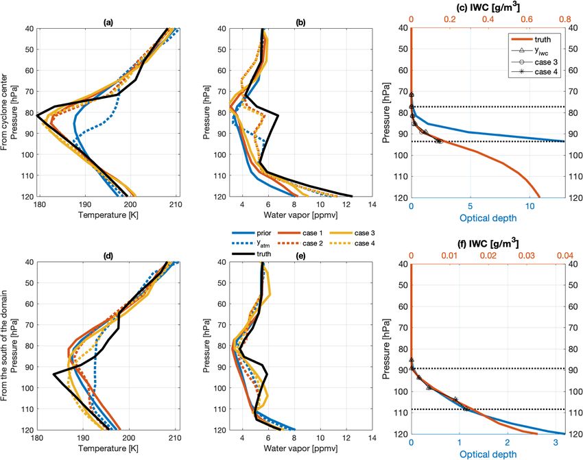
constraints to improve the precision of the method. Furthermore, individual profiles from two clusters of over-
The results for Case 1 are shown as solid red curves in shooting DCCs, which include the DCCs near the cyclone
Figs. 5 and 7. The major improvement in Case 1 as com- center and those in the south of the domain, are randomly
pared to the prior (solid blue curves) is in the temperature selected to investigate how well the retrieval reproduces the
profile from 100 to 75 hPa. Although the DFS for water va- spatial variability in temperature and water vapor. The all-sky
por reaches 0.69, Case 1 does not provide much of an im- optical depths from TOA and IWC profiles for the two loca-
provement in water vapor from the first guess. tions are shown in Fig. 7c, d. The retrievable signals mainly
Case 2 improves upon Case 1 owing to the informa- come from the atmospheric column above thick cloud layers,
tion carried by the additional atmospheric constraints, y atm . i.e., where the optical depth is less than 2 (only 13.5 % of the
Case 2 is represented by the dotted red curves in Figs. 5 and infrared emission is transmitted through this cloud layer).
7. It approaches the true state better than Case 1, despite Figure 7a–c shows results for a location close to the cy-
warm and dry biases in the first guess and y atm (see Fig. 5a, clone center. At this location, the slab-cloud method pre-
c). Notably, it increases the retrieved water vapor concentra- scribes the cloud layer to be located at the cold point due
tion by around 1 ppmv on average and reduces the RMSE to the strong cloud emission. Atmospheric anomalies above
from 2.4 to 1.0 ppmv, as shown in Fig. 5c, d and Table 2. 86 hPa have an impact on TOA infrared radiances. Around
Atmos. Meas. Tech., 14, 5717–5734, 2021 https://doi.org/10.5194/amt-14-5717-2021You can also read