Mass, nutrients and dissolved organic carbon (DOC) lateral transports off northwest Africa during fall 2002 and spring 2003
←
→
Page content transcription
If your browser does not render page correctly, please read the page content below
Ocean Sci., 16, 483–511, 2020
https://doi.org/10.5194/os-16-483-2020
© Author(s) 2020. This work is distributed under
the Creative Commons Attribution 4.0 License.

Mass, nutrients and dissolved organic carbon (DOC) lateral
transports off northwest Africa during fall 2002
and spring 2003
Nadia Burgoa1 , Francisco Machín1 , Ángeles Marrero-Díaz1 , Ángel Rodríguez-Santana1 , Antonio Martínez-Marrero2 ,
Javier Arístegui2 , and Carlos Manuel Duarte3
1 Departamento de Física, Universidad de Las Palmas de Gran Canaria, Las Palmas de Gran Canaria, Spain
2 Instituto
          de Oceanografía y Cambio Global, Universidad de Las Palmas de Gran Canaria, Telde, Spain
3 Red Sea Research Center, King Abdullah University of Science and Technology, Thuwal, Saudi Arabia

Correspondence: Nadia Burgoa (nadia.burgoa@ulpgc.es)

Received: 29 July 2019 – Discussion started: 26 August 2019
Revised: 6 March 2020 – Accepted: 12 March 2020 – Published: 24 April 2020

Abstract. The circulation patterns and the impact of the lat-      1   Introduction
eral export of nutrients and organic matter off NW Africa are
examined by applying an inverse model to two hydrographic          The North Atlantic subtropical gyre (NASG) is one of the
datasets gathered in fall 2002 and spring 2003. These esti-        most important components in the thermohaline circulation.
mates show significant changes in the circulation patterns at      It presents a well-known intensification in its western mar-
central levels from fall to spring, particularly in the southern   gin, the Gulf Stream, with maximum velocities up to 2 m s−1
boundary of the domain related to zonal shifts of the Cape         (Halkin and Rossby, 1985). The currents observed in this
Verde Frontal Zone. Southward transports at the surface and        western margin of the gyre occupy a small horizontal ex-
central levels at 26◦ N are 5.6 ± 1.9 Sv in fall and increase      tension compared to that of the currents in the eastern side,
to 6.7 ± 1.6 Sv in spring; westward transports at 26◦ W are        resulting in an asymmetric gyre (Stramma, 1984; Tomczak
6.0 ± 1.8 Sv in fall and weaken to 4.0 ± 1.8 Sv in spring. At      and Godfrey, 2003). The low intensity of the currents at
21◦ N a remarkable temporal variability is obtained, with a        the eastern boundary made them very little studied until the
northward mass transport of 4.4 ± 1.5 Sv in fall and a south-      1970s, when the CINECA (Cooperative Investigations of the
ward transport of 5.2 ± 1.6 Sv in spring. At intermediate lev-     Northern Part of the Eastern Central Atlantic) program fo-
els important spatiotemporal differences are also observed,        cused on the productive African upwelling system (Ekman,
and it must be highlighted that a northward net mass transport     1923; Tomczak, 1979; Hughes and Barton, 1974; Hempel,
of 2.0 ± 1.9 Sv is obtained in fall at both the south and north    1982). Käse and Siedler (1982) found strikingly intense cur-
transects. The variability in the circulation patterns is also     rents south of the Azores connected to the Gulf Stream and
reflected in lateral transports of inorganic nutrients (SiO2 ,     suggested that part of the recirculation of the NASG occurs
NO3 , PO4 ) and dissolved organic carbon (DOC). Hence, in          southward in the vicinity of the African coast. Later on, sev-
fall the area acts as a sink of inorganic nutrients and a source   eral surveys based on both in situ and remote sensing obser-
of DOC, while in spring it reverses to a source of inorganic       vations contributed to defining the general characteristics
nutrients and a sink of DOC. A comparison between nutrient         for the average flow of the region (Käse and Siedler, 1982;
fluxes from both in situ observations and numerical modeling       Stramma, 1984; Käse et al., 1986; Stramma and Siedler,
output is finally addressed.                                       1988; Mittelstaedt, 1991; Zenk et al., 1991; Fiekas et al.,
                                                                   1992; Hernández-Guerra et al., 1993).
                                                                      Most of the eastward flow from the Gulf Stream is con-
                                                                   fined to a band between the Azores and Madeira islands, re-
                                                                   circulating southward through the Canary Islands and north

Published by Copernicus Publications on behalf of the European Geosciences Union.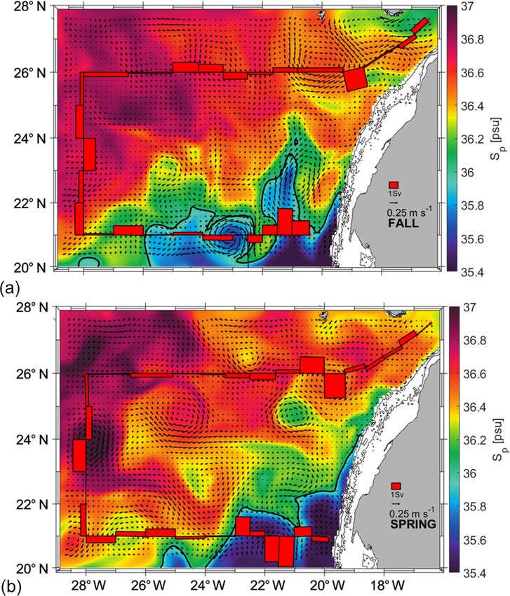
484                                            N. Burgoa et al.: Mass, nutrients and DOC lateral transports off NW Africa

of Cape Verde to become a southwestward flow (Stramma,            and biogeochemical processes. Within the euphotic zone, pri-
1984). This current system is composed of the Azores Cur-         mary production is solely limited by the availability of inor-
rent (AC), the Canary Current (CC), the Canary Upwelling          ganic nutrients (INs) (Copin-Montegut and Copin-Montegut,
Current (CUC), the North Equatorial Current (NEC) and the         1983; Falkowski et al., 1998). Below the euphotic zone res-
Poleward Undercurrent (PUC). The AC divides into several          piration exceeds primary production. As a result, the organic
branches defining the boundary current system off north-          matter produced at the sea surface is remineralized in the sub-
west Africa. It first feeds the Iberian Current (Haynes et al.,   surface layers, and hence the concentration of INs increases
1993), while a second significant branch enters the Mediter-      from the interplay between the local rate of remineralization
ranean Sea (Candela, 2001). Most of the AC recirculates           and the rate of water supply (Azam, 1998; Del Giorgio and
southward, splitting into the main CC across the Canarian         Duarte, 2002; Pelegrí et al., 2006; Pelegrí and Benazzouz,
archipelago and the secondary CUC (Pelegrí et al., 2005,          2015b).
2006). These currents extend southward, developing the               In order to study the impact of lateral transports on the dis-
Cape Verde Frontal Zone (CVFZ), a density-compensated             tributions of biogeochemical variables, the first step to fol-
front with North Atlantic Central Water at its northern side      low is to analyze the dynamic of the area with an inverse
and South Atlantic Central Water at its southern one (Zenk        box model. This method provides a velocity field consistent
et al., 1991; Martínez-Marrero et al., 2008). Finally, the        with both mass and property conservation within a closed
PUC is located below the CUC, flowing northward on the            volume and with the thermal wind equation (Wunsch, 1996).
continental slope (Barton, 1989; Machín and Pelegrí, 2009;        Several authors have already described the circulation pat-
Machín et al., 2010; Pelegrí and Peña-Izquierdo, 2015).           terns of the NASG by applying an inverse model (Ganachaud
   Mesoscale activity constitutes a second main feature in        and Wunsch, 2002; Ganachaud, 2003b, a; Hernández-Guerra
the area of interest, which might be even more energetic          et al., 2005, 2017; Machín et al., 2006; Pérez-Hernández
than the average flow itself (Sangrà et al., 2009). Three         et al., 2013). Moreover, some recent papers addressing lat-
mesoscale domains may be defined: the Canary Eddy Cor-            eral advective transports of biogeochemical variables have
ridor (CEC; Sangrà et al., 2009), the CVFZ and the up-            shed light on this topic in the EBUS off NW Africa (Álvarez
welling front. The CEC is located downstream of the Canary        and Álvarez-Salgado, 2009; Alonso-González et al., 2009;
Islands where the interaction between the southward flow          Santana-Falcón et al., 2017; Fernández-Castro et al., 2018).
and the archipelago generates long-lived eddies (Arístegui           To sum up, the main goal of this paper is to present an
et al., 1994; Barton et al., 1998; Sangrà et al., 2007, 2009;     in situ hydrographic database and to estimate lateral mass as
Ruiz et al., 2014; Barceló-Llull et al., 2017a). The second       well as IN and DOC transports during fall and spring seasons
mesoscale domain is the CVFZ, where several meanders              south of the Canary Islands in the context of a highly variable
and eddies produce strong interleaving between the water          environment featured by the Canary Eddy Corridor, the up-
masses involved (Pérez-Rodríguez et al., 2001; Martínez-          welling off northwest Africa and the CVFZ. The remainder
Marrero et al., 2008). In this domain, the CC and the CUC         of this paper is organized as follows: the dataset is presented
separate from the African coast, fueling the NEC and giv-         in Sect. 2; the seasonal distribution of the water masses and
ing rise to a shadow zone featured by poorly ventilated wa-       their properties is displayed in Sect. 3; the technical details
ters (Luyten et al., 1983). The third area is the front arising   of the inverse box model are covered in Sect. 4; and the re-
between the coastal upwelled waters and the stratified inte-      sulting velocity field and the corresponding mass, nutrient
rior waters, defining the Eastern Boundary Upwelling Sys-         and organic matter transports are presented in Sect. 5. Sec-
tem (EBUS) in the northwest African region (Mittelstaedt,         tion 6 is devoted to the discussion, with some conclusions in
1983; Pastor et al., 2008; Arístegui et al., 2009). This EBUS     Sect. 7.
is actually located off the African slope from the Gulf of
Cádiz until Cape Blanc–Cape Verde in summer–winter with
high mesoscale variability in the form of both filaments and      2   Dataset
eddies (Hagen, 2001; Sangrà et al., 2009; Ruiz et al., 2014).
The upwelling process raises nutrient-rich waters to the eu-      The COCA-I and COCA-II cruises were carried out in fall
photic layer, developing a high-primary-production latitudi-      (10 September to 1 October 2002) and spring (21 May to
nal band off northwest Africa known as the Coastal Transi-        7 June 2003), respectively, aboard the BIO Hesperides as
tion Zone (CTZ) (Barton et al., 1998; Pelegrí et al., 2006).      part of the research project Coastal-Ocean Carbon Exchange
These mesoscale features play an essential role as a lateral      in the Canary Region (Hernández-León et al., 2019). The lo-
source of organic matter towards the oligotrophic waters of       cation of conductivity–temperature–depth (CTD), inorganic
the NASG (Barton et al., 1998; García-Muñoz et al., 2004,         nutrient (IN) and dissolved organic carbon (DOC) stations
2005; Pelegrí et al., 2006; Álvarez-Salgado et al., 2007; San-    in COCA-I and COCA-II defines a closed box along three
grà et al., 2009).                                                transects (Fig. 1). The northern transect (N) spans from sta-
   The distribution of inorganic nutrients and organic mat-       tion 1 to 32 at 26◦ N (the section from stations 1 to 11 is
ter in the ocean responds to a combined effect of physical        tilted some 30◦ with respect to the east). The western tran-

Ocean Sci., 16, 483–511, 2020                                                                 www.ocean-sci.net/16/483/2020/
N. Burgoa et al.: Mass, nutrients and DOC lateral transports off NW Africa                                                   485

Table 1. Summary of the number and type of measurements at sta-     centrated in the shallowest layers (< 200 m; Fig. 2, pink
tions per transect and season.                                      crosses).
                                                                       Wind data were selected from the QuikSCAT database
  Season       Type of                 Number of stations           made available by CERSAT (Centre ERS d’ Archivage et de
  (cruise)     measurement                                          Traitement; http://www.ifremer.fr/cersat/ (last access: 20 De-
                               North     West    South      Total   cember 2017). These wind fields were averaged weekly with
                                                                    a spatial resolution of 0.5◦ (shown in Fig. 1 with half of the
  Fall         CTD                14       6        11       29
                                                                    original spatial resolution). The Smith–Sandwell database
  (COCA-I)     INs                 8       2         6       14
               DOC                 8       2         6       15     with 1 min horizontal resolution was used as the source of
                                                                    bathymetry data (Smith and Sandwell, 1997).
  Spring       CTD                15       6        12       31        Freshwater flux data were estimated from the rates of
  (COCA-II)    INs                 9       3         8       18
                                                                    evaporation and precipitation extracted from the Surface Ma-
               DOC                10       3         7       18
                                                                    rine Data 1994 of da Silva et al. (1994) (http://iridl.ldeo.
                                                                    columbia.edu/SOURCES/.DASILVA/.SMD94/, last access:
                                                                    20 December 2017). The climatological mean depths of the
                                                                    neutral density field for the years 2002 and 2003 were cal-
sect (W) is located at 26◦ W from station 32 to 42. Finally,        culated from the climatological temperature and salinity ex-
the southern zonal transect (S) at 21◦ N runs from station 42       tracted from the World Ocean Atlas 2013 (WOA13; https:
to 63 (COCA-I) or 66 (COCA-II) over the continental slope           //www.nodc.noaa.gov/OC5/woa13/woa13data.html, last ac-
(Table 1). The distance between neighboring CTD stations            cess: 1 February 2018, Locarnini et al., 2013; Zweng et al.,
was some 50 km except for the stations over the continental         2013).
slope where this distance was shortened. Adjacent DOC and              GLORYS         (GLOBAL_REANALYSIS_PHY_001_025
IN stations were separated by a variable distance, with the         product) issued by the Copernicus Marine Environment
shortest distance being about 50 km at stations closer to the       Monitoring Service (CMEMS; http://marine.copernicus.eu,
coast.                                                              last access: 5 June 2018, Garric and Parent, 2018) was used
   CTD data were collected from the sea surface down to             as a primary source of dynamic variables. Its horizontal
2000 m of depth with a vertical resolution of 2 dbar. In situ       resolution is 1/12◦ with 50 standard depths. Hydrological
temperature was calibrated with 45 readings performed with          data from GLORYS were also employed to diagnose the
a reversible digital thermometer, while salinity was cali-          average oceanographic conditions during each cruise. This
brated by analyzing 60 water samples with the Portasal sali-        product assimilates field observations in real time.
nometer. The residuals have an average value of 0.00013 ±              The                    SEALEVEL_GLO_PHY_L4_REP_
0.00400 ◦ C and 0.0005 ± 0.005 in salinity.                         OBSERVATIONS_008_047 product provided surface
   DOC was measured with a total organic carbon (TOC) an-           geostrophic currents estimated from sea level anomalies.
alyzer (Shimadzu TOC-5000), assuming that almost all TOC            These data capture the mesoscale structures and are helpful
was in dissolved form. Water samples (10 mL) were dis-              to validate the near-surface geostrophic field estimated from
pensed directly into glass ampoules previously combusted            the inverse model.
at 500 ◦ C during 12 h; 50 µL of H3 PO4 was immediately                GLORYS-BIO (GLOBAL_REANALYSIS_BIO_001_029
added to the sample, sealed and stored at 4 ◦ C until ana-          product) produced daily mean 3D biogeochemical fields
lyzed. Before the analysis, samples were sparged with CO2 -         with the same resolution as GLORYS. This reanalysis forces
free air for several minutes to remove inorganic carbon. TOC        the biogeochemical model with the nutrient initial conditions
concentrations were determined from standard curves (30             from WOA13. IN concentrations from GLORYS-BIO (SiO2 ,
to 200 µM) of potassium hydrogen phthalate produced ev-             NO3 , and PO4 ) were used to assess nutrient transports by
ery day (Thomas et al., 1995). To check accuracy and pre-           the model (in Sect. 5).
cision, reference material from the Jonathan H. Sharp lab-             The data treatment, the graphical representations and the
oratory (University of Delaware) was analyzed daily. DOC            inverse model are coded in MATLAB (MATLAB, 2018). The
distribution up to 2000 m of depth presented more represen-         vertical sections are produced using the “nearest” 2D inter-
tative coverage in fall than in spring (Fig. 2, green dots), de-    polations, a method also employed in the estimates of the
spite the number of stations being higher in spring than in         IN and DOC transports. Ocean Data View using the DIVA
fall (Fig. 1, black circles; Table 1).                              gridding method is employed to produce DOC concentration
   The three inorganic nutrients sampled were silicates             charts (Schlitzer, 2019).
(SiO2 ), nitrates plus nitrites (NOx ) and phosphates (PO4 ).
These samples were frozen until measured with a
Bran+Luebbe AA3 autoanalyzer following the standard
methodology established by Hansen and Koroleff (1999).
Nutrient data covered up to 2000 m, while in fall they con-

www.ocean-sci.net/16/483/2020/                                                                   Ocean Sci., 16, 483–511, 2020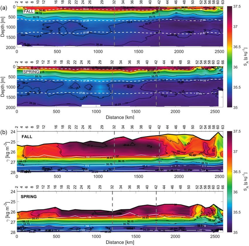
486 N. Burgoa et al.: Mass, nutrients and DOC lateral transports off NW Africa
Figure 1. Hydrological (red dots), inorganic nutrient (pink circles) and DOC (black circles) sampling stations during the COCA-I (a) and
COCA-II (b) cruises. Time-averaged wind stress during each cruise is also represented by the inset arrow denoting the scale (shown with
half of the original spatial resolution).
3 Hydrography and water masses east of the domain. The N–W and W–S corners are indicated
with two vertical grey dashed lines at stations 32 and 42, re-
spectively.
Neutral density γn = γn (θ, S, p) is used as the density ref- The 2 − SA diagrams exhibit four regions delimited by
erence variable, with the isoneutrals representing the sur- potential density anomaly contours of 26.39, 27.30 and
faces where the values of γn are constant (Jackett and Mc- 27.72 kg m−3 , equivalent to the isoneutrals that separate the
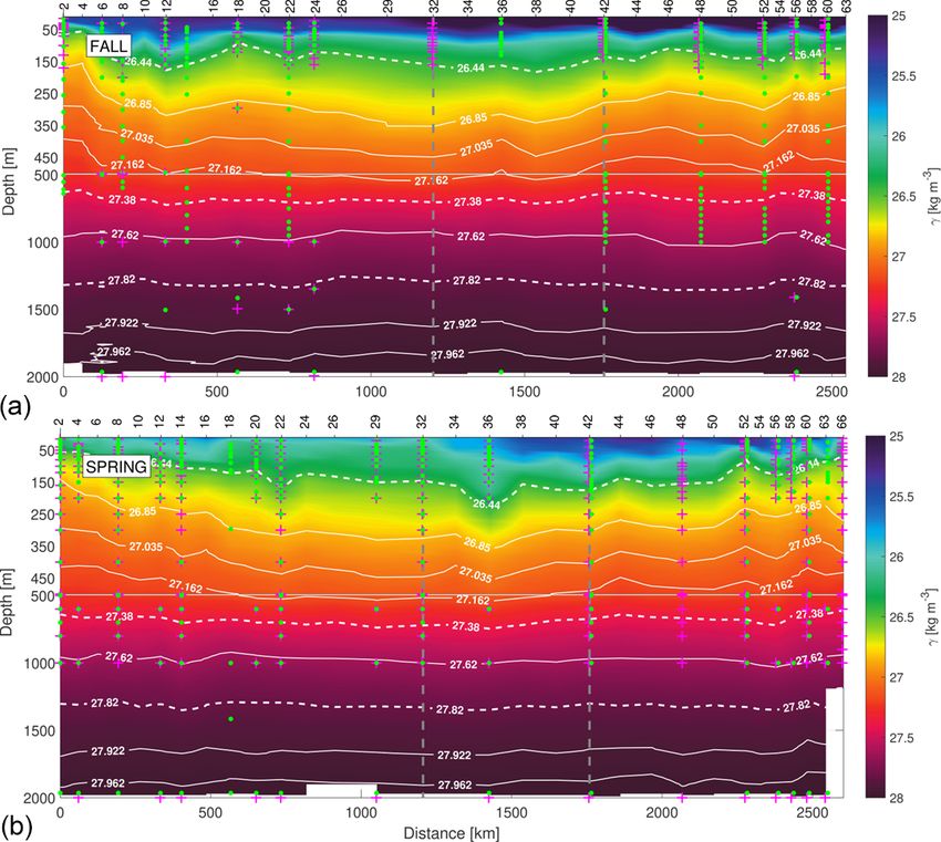
Dougall, 1997). The γn vertical sections contain the surface main water masses (Fig. 3). These three isoneutrals are ap-
(SW), central (CW), intermediate (IW) and deepwater (DW) proximately at 132–123, 672–700 and 1294–1305 m of depth
masses according to Macdonald (1998) for the North Atlantic (Fig. 2). The water masses sampled during both cruises are
at 24◦ N, represented with white dashed lines at 26.44, 27.38 North Atlantic Central Water (NACW), South Atlantic Cen-
and 27.82 kg m−3 (Fig. 2). The x-axis direction is selected tral Water (SACW), Antarctic Intermediate Water (AAIW),
according to the path followed by the vessel during both Mediterranean Water (MW) and North Atlantic Deep Wa-
cruises, starting in the northeast and finishing in the south-
Ocean Sci., 16, 483–511, 2020 www.ocean-sci.net/16/483/2020/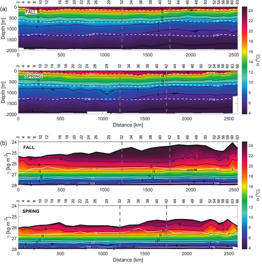
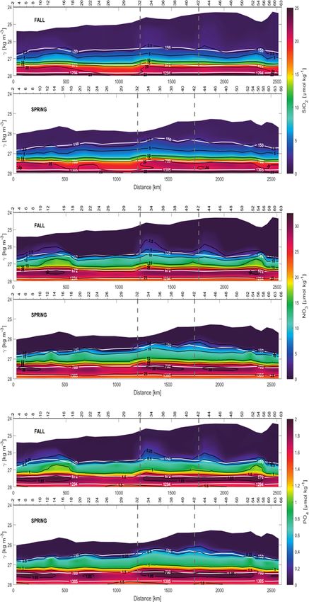
N. Burgoa et al.: Mass, nutrients and DOC lateral transports off NW Africa                                                                    487

Figure 2. The γn vertical sections during fall (a) and spring (b) cruises. White dashed isoneutrals limit the different water type layers. The
direction chosen for the representation of the transects is the course of the vessel. Distance is calculated with respect to the first station (2).
The section is divided into three transects: the northern transect from east to west (from station 2 to 32), the western transect from north to
south (from station 32 to 42) and the southern transect from west to east (from stations 42 to 63–66). The three transects are separated by
two vertical grey dashed lines located at stations 32 and 42. The sampling points of INs and DOC used in this work are also represented by
pink crosses and green dots, respectively.

ter (NADW) (Emery and Meincke, 1986; Macdonald, 1998;                          A description of the temporal variability of the water
Emery, 2001). Their main hydrological characteristics are                   masses is also given with observations from the 2 − SA dia-
summarized in Table 2. Below the mixing layer and above                     grams (Fig. 3). The distribution of water masses is quite sim-
700 m (26.44 < γn < 27.38 kg m−3 ), NACW and SACW are                       ilar for both cruises. There is a higher temperature variability
the dominant water masses. SACW is featured by a higher                     at the surface waters during fall, with maximum values 2–
amount of nutrients, and it is 1–2 ◦ C colder and 0.1–0.4                   3 ◦ C higher than in spring. During spring, the variability ob-
fresher than NACW (Fig. 3 and Table 2). Below, from 700                     served at central waters is associated with larger fluctuations
up to 1300 m (27.38 < γn < 27.82 kg m−3 ), the intermedi-                   in salinity affecting the whole water column. At DW there is
ate waters AAIW and MW are the dominant water masses                        a higher contribution of NADW in the whole domain during
(Hernández-Guerra et al., 2017). MW is a relatively warm                    fall. Finally, the surface layer is thicker in fall than in spring
and salty water mass, while AAIW is colder and fresher (Ta-                 in all the sections made with respect to γn .
ble 2). Finally, below 1300 m (γn > 27.82 kg m−3 ) the pre-                    These temporal differences may also be described transect
dominant water mass is NADW, with in situ temperature and                   to transect. The northern transect (Fig. 2, stations 2 to 32;
salinity values lower than 5.7 ◦ C and 35.14 (Table 2).                     Fig. 3, magenta dots) is occupied by NACW, AAIW, MW

www.ocean-sci.net/16/483/2020/                                                                                Ocean Sci., 16, 483–511, 2020
488                                                N. Burgoa et al.: Mass, nutrients and DOC lateral transports off NW Africa

Table 2. Summary of water levels (CW, IW and DW) with their isoneutral limits and their water mass properties for both seasons from
the sea surface to 2000 m. The properties extracted from observations are in situ temperature (T ), potential temperature (θ ), conservative
temperature (2), practical salinity (SP ), absolute salinity (SA ) and dissolved organic carbon (DOC). The INs extracted from GLORYS-BIO
are silicates (SiO2 ), nitrates (NO3 ) and phosphates (PO4 ).

                    Water levels                      CW                                          IW                             DW
                                           Min.               Max.                 Min.                   Max.            Min.     Max.
                    γn (kg m−3 )
                                           26.44              27.38                27.38                  27.82          27.82    27.962
                    Water masses          NACW                SACW                  MW                    AAIW              NADW
            Properties        Season   Min.      Max.      Min.    Max.         Min.    Max.           Min.    Max.      Min.         Max.
            T                 fall      9.12    19.13       8.22   17.18         6.03   10.02           5.25      9.12    3.63         5.66
            (◦ C)             spring    5.90    19.76       8.35   17.14         6.01   10.04           5.16      9.41    3.63         5.57
            θ                 fall      9.04    19.11       8.14   17.16         5.90      9.94         5.13      9.05    3.46         5.53
            (◦ C)             spring    5.77    19.74       8.27   17.13         5.88      9.96         5.06      9.34    3.47         5.45
            2                 fall      9.03    19.05       8.13   17.12         5.89      9.92         5.12      9.03    3.46         5.53
            (◦ C)             spring    5.77    19.67       8.26   17.09         5.88      9.94         5.05      9.32    3.47         5.44
            SP                fall     35.23    36.83      35.04   36.19       35.13    35.44          34.92   35.24     34.99        35.13
                              spring   33.85    37.06      35.07   36.16       34.55    35.53          34.96   35.30     34.99        35.12
            SA                fall     35.40    37.00      35.21   36.36       35.30    35.61          35.09   35.40     35.16        35.30
            (g kg−1 )         spring   34.02    37.23      35.24   36.33       34.72    35.70          35.13   35.47     35.16        35.30
            SiO2              fall      1.24    18.46       6.39   22.14       13.23    21.73          17.50   25.78     18.94        28.44
            (µmol kg−1 )      spring    1.22    21.99       6.99   23.95       13.97    21.99          17.97   28.06     19.04        28.73
            NO3               fall      0.00    30.27      22.03   36.15       23.13    30.92          25.82   36.36     20.55        28.26
            (µmol kg−1 )      spring    0.00    30.36      25.21   36.75       23.78    31.18          25.70   36.81     21.06        27.97
            PO4               fall      0.03       1.90     1.46      2.29       1.43      1.98         1.69      2.33    1.37         1.85
            (µmol kg−1 )      spring    0.03       1.90     1.69      2.36       1.49      1.98         1.69      2.39    1.42         1.83
            DOC               fall     47.85   108.65      49.05   74.13       46.25    66.09          41.83   59.30     41.82        58.72
            (µM)              spring   41.66   105.62      40.86   63.45       40.44    65.15          40.44   50.17     40.44        50.81

and NADW in both seasons. At intermediate levels, a higher                   MW is registered at the northern transect, while in the south-
contribution of MW is observed in spring, while a slightly                   ern one the predominant water mass is AAIW. Regarding the
higher contribution of AAIW is obtained in fall. The western                 seasonal variability, the contribution of MW in the northern
transect (Fig. 2, stations 32 to 42; Fig. 3, dark grey dots) has a           transect is higher in spring, while the contribution of AAIW
similar distribution as the northern one, with a lower variabil-             in the southern transect is higher in fall.
ity in the upper layers and a smaller influence of MW. In the                   Although the INs have been extracted from the model and
southern transect (Fig. 2, stations 42 to 63–66; Fig. 3, blue                the distributions of 2, SA and γn have been obtained from
dots), the highest spatiotemporal variability is observed. This              the hydrographic observations, there is a good agreement be-
variability at the surface and central levels is associated with             tween the structures described by both datasets. The in situ
the position of the CVFZ and, in turn, with the mesoscale                    concentrations of SiO2 , NOx and PO4 up to 250 m of depth
and submesoscale structures associated with the front. The                   (black dots in Fig. 6) are represented together with the time-
CVFZ is located where the isohaline of 36, or equivalently                   averaged concentrations of SiO2 , NO3 and PO4 up to 2000 m
SA = 36.15 g kg−1 , intersects the 150 m isobath (Zenk et al.,               of depth selected from GLORYS-BIO. In this way the IN out-
1991) (Fig. 4). CVFZ is found in the southern transect in                    puts from the model are compared with in situ observations
its westernmost position in fall, at stations 46–48. Hence,                  since their concentration in both cases presents an acceptable
SACW with relatively low SA is observed above the upper                      match, with the exception of NOx and PO4 concentrations at
limit of CW east of the CVFZ location (Fig. 4). In spring,                   the S transect. On the other hand, the IN model outputs look
the CVFZ shifts to a position closer to the African coast at                 like INs from historical in situ databases (not shown here).
station 52, with a water incursion of higher-salinity NACW                      At central levels, high IN concentrations have been sam-
centered at station 58 (Figs. 4 and 5). At intermediate levels,              pled near the continental slope in both the northern (sta-

Ocean Sci., 16, 483–511, 2020                                                                                  www.ocean-sci.net/16/483/2020/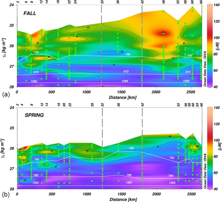
N. Burgoa et al.: Mass, nutrients and DOC lateral transports off NW Africa                                                          489

                                                                         to the CVFZ (Zenk et al., 1991; Sangrà et al., 2009). IN con-
                                                                         centrations are notably high at intermediate and deep levels
                                                                         compared to those at central levels (Fig. 6) and have the same
                                                                         order of magnitude as those documented before in the do-
                                                                         main (Pérez et al., 2001; Pérez-Hernández et al., 2013). The
                                                                         distributions of SiO2 , NO3 and PO4 are similar during both
                                                                         cruises, and their concentrations increase with depth as a re-
                                                                         sult of the remineralization of organic matter (Fig. 7). The
                                                                         area where the least nutrients are found at depth throughout
                                                                         the domain is the northwest corner of the box (stations 24
                                                                         to 32). With respect to the IN seasonal variability at inter-
                                                                         mediate depths, the three concentrations do not present large
                                                                         differences between the values measured in fall and spring
                                                                         (Figs. 7 and 3). In both seasons the concentrations of SiO2 ,
                                                                         NO3 and PO4 are 4–6, 2–6 and 0.2–0.4 µmol kg−1 higher in
                                                                         AAIW than in MW (Table 2). The NADW is characterized
                                                                         by a moderate increase in SiO2 and a slight decrease in NO3
                                                                         and PO4 with respect to the values documented here at in-
                                                                         termediate levels. In both seasons, the maximum concentra-
                                                                         tion of SiO2 is 28–29 µmol kg−1 . Nevertheless, specifically
                                                                         in spring, the maximum concentrations of NO3 and PO4 , 28
                                                                         and 1.8–1.9 µmol kg−1 , are lower than those recorded at in-
                                                                         termediate levels, providing a similar vertical variability as
                                                                         that reported by Machín et al. (2006) (Table 2).
                                                                            DOC concentrations are higher and more widely dis-
                                                                         tributed in the water column in fall than in spring, when
                                                                         the DOC maximum values are more confined to surface and
                                                                         central waters (Figs. 8 and 6, Table 2). This fact is espe-
                                                                         cially significant in the southern transect occupied by SACW
                                                                         (Fig. 6). SACW presents maximum concentrations of DOC
                                                                         35–40 µmol L−1 lower than those found for NACW (Table 2).
                                                                         This difference is more pronounced in spring (Table 2). In
                                                                         addition, the fall DOC observations present a larger variabil-
                                                                         ity in central waters, as previously seen for INs. Lower DOC
                                                                         concentrations are observed for stations sampled in the west-
                                                                         ern transect, while the highest concentrations are recorded
                                                                         in the stations next to the African slope with values above
                                                                         100 µmol L−1 (Fig. 8). On the other hand, the high concentra-
                                                                         tions of DOC recorded at intermediate waters in the northern
                                                                         transect during both cruises are noteworthy (Figs. 8 and 6).

Figure 3. 2 − SA diagrams of hydrological measurements during
the fall (a) and spring (b) cruises. The different water masses at the   4   The inverse model
north (N, magenta dots), west (W, dark grey dots) and south (S, blue
dots) transects are SW, NACW, SACW, AAIW, MW and NADW.                   An inverse box model is applied to the hydrographic data
Potential density anomaly contours equivalent to the 26.44, 27.38        from the two COCA cruises to provide the absolute velocity
and 27.82 kg m−3 isoneutrals delimit the surface, central, interme-      field across the three sections (Wunsch, 1978). This method
diate and deepwater levels.                                              has been widely applied in different areas of the Atlantic
                                                                         Ocean as an efficient method to obtain absolute geostrophic
                                                                         flows (Martel and Wunsch, 1993; Paillet and Mercier, 1997;
tions 10 to 18) and southern (50 to 56) transects in fall.               Ganachaud, 2003a; Machín et al., 2006; Pérez-Hernández
The values observed are 1–5 µmol kg−1 for NO3 and 0.1–                   et al., 2013; Hernández-Guerra et al., 2017; Fu et al., 2018).
0.4 µmol kg−1 for PO4 , which are higher values than those               Assuming geostrophy and the conservation of mass and other
recorded in spring at similar places (Fig. 7). This might be             properties in the ocean bounded by the African coast and the
related to long-lived mesoscale eddies or instabilities related          hydrological sections, the velocity fields are obtained, allow-

www.ocean-sci.net/16/483/2020/                                                                         Ocean Sci., 16, 483–511, 2020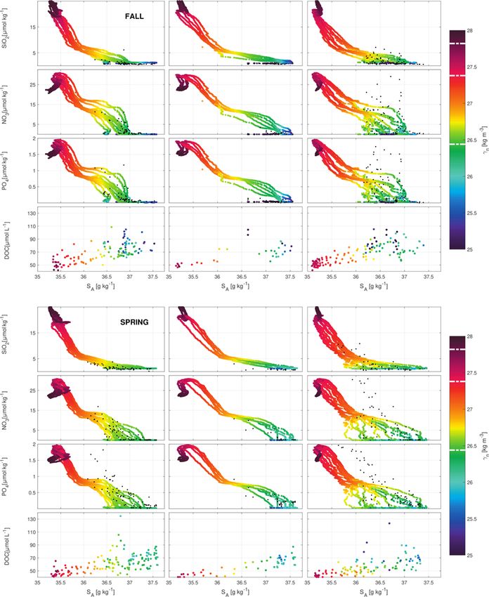
490                                                 N. Burgoa et al.: Mass, nutrients and DOC lateral transports off NW Africa

Figure 4. Sections of absolute salinity (SA ) with respect to depth (a) and γn (b) during fall and spring. In the depth section in panel (a), the
isoneutrals that delimit the transports at the surface, central, intermediate and deep water are represented by white dashed contours. In the γn
section (b), the depths of 150, 672–700 and 1294–1305 m are also shown.

ing for an adjustment of freshwater flux and Ekman trans-                  represented in Fig. 2. The upper five layers group the sur-
ports.                                                                     face and central waters, and the first layer until the isoneutral
                                                                           26.44 kg m−3 is related to surface waters, while the four re-
4.1   Selection of layers                                                  maining layers between 26.44 and 27.38 kg m−3 are central
                                                                           waters. The intermediate waters are found in the next two
The closed ocean where the inverse model is applied is di-                 layers between 27.38 and 27.82 kg m−3 , while the deepest
vided into nine layers by means of the neutral densities                   two layers below 27.82 kg m−3 contain the upper deep wa-
defined by Macdonald (1998) and modified by Ganachaud                      ters.
(2003a) for the North Atlantic Ocean. This distribution is
then slightly modified to include two layers instead of one                4.2   The system of equations
between 26.85 and 27.162 kg m−3 by adding the isoneutral
27.035 kg m−3 , as other authors have done previously at this              The inverse box model takes into account mass conservation
side of the NASG (Comas-Rodríguez et al., 2011; Pérez-                     per layer and also in the whole water column. The salinity
Hernández et al., 2013). The locations of the isoneutrals are              is actually introduced as a salinity anomaly, which is also

Ocean Sci., 16, 483–511, 2020                                                                             www.ocean-sci.net/16/483/2020/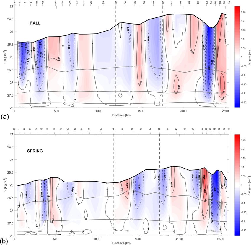
N. Burgoa et al.: Mass, nutrients and DOC lateral transports off NW Africa                                                                491

Figure 5. Sections of conservative temperature (2) with respect to depth (top) and γn (bottom) during fall and spring. In the depth section in
panel (a), the isoneutrals that delimit the transports at the surface, central, intermediate and deep water in the water column are represented
by white dashed contours. In the γn section (b), the depths of 150, 672–700 and 1294–1305 m are indicated.

conservative within individual layers and in the whole water              the Ekman transport adjustments (one unknown per section)
column (Ganachaud, 2003b). On the other hand, heat is in-                 and 1 unknown for the freshwater flux. The resulting sys-
troduced as a heat anomaly in the two deepest layers wherein              tem is undetermined and a Gauss–Markov estimator is used
it is also considered conservative. The salinity and heat are             to select a solution by adding a priori information. This a
added as anomalies to improve the conditioning of the in-                 priori information consists of the uncertainties for both the
verse model and get a higher rank in the system of equa-                  unknowns (Rxx ) and the noise of the equations (Rnn ).
tions by reducing the linear dependency between equations
(Ganachaud, 2003b).                                                       4.2.1   Uncertainties of unknowns (Rxx )
   Therefore, the model is composed of a set of 22 equa-
tions (10 for mass conservation, 10 for salt anomaly conser-
                                                                          The geostrophic velocity field is calculated in the central po-
vation and 2 for heat anomaly conservation). Those equa-
                                                                          sition between two consecutive stations. The isoneutral se-
tions are solved for 32 and 34 unknowns, comprised of 28–
                                                                          lected as the reference level is the deepest common γn for
30 reference-level velocities in fall–spring, 3 unknowns for
                                                                          all the stations, 27.962 kg m−3 (Fig. 2). Initially, the ref-

www.ocean-sci.net/16/483/2020/                                                                             Ocean Sci., 16, 483–511, 2020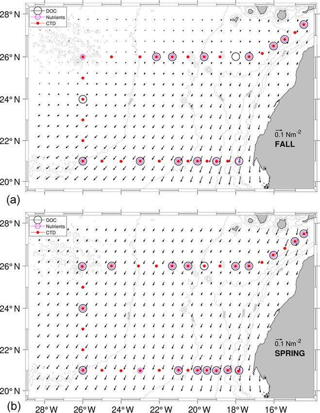
492                                                N. Burgoa et al.: Mass, nutrients and DOC lateral transports off NW Africa

Figure 6. Scatter plots for SiO2 , NO3 and PO4 nutrients (µmol kg−1 ; extracted from GLORYS-BIO), as well as for DOC (observational
data: µmol L−1 ) with respect to SA and γn at the north (left), west (middle) and south transects (right) in fall (top) and spring (bottom). The
isoneutrals 26.44, 27.38 and 27.82 kg m−3 that limit the waters layers are indicated with white dashed lines in the color bar. The measured
IN concentrations (µmol kg−1 ) for SiO2 , NOx and PO4 until 250 m of depth are included as black dots.

Ocean Sci., 16, 483–511, 2020                                                                            www.ocean-sci.net/16/483/2020/
N. Burgoa et al.: Mass, nutrients and DOC lateral transports off NW Africa                                                         493

Figure 7. Sections for SiO2 (top), NO3 (middle) and PO4 (bottom) concentrations with respect to γn during fall (top) and spring (bottom)
extracted from GLORYS-BIO. The white isolines are as in the γn sections in Figs. 4 and 5.

www.ocean-sci.net/16/483/2020/                                                                        Ocean Sci., 16, 483–511, 2020
494                                              N. Burgoa et al.: Mass, nutrients and DOC lateral transports off NW Africa

Figure 8. Sections of DOC concentration with respect to γn during the fall (a) and spring (b) cruises with the white isolines as in the γn
sections in Figs. 4 and 5.

erence level is considered a motionless level at which the             and the variability of the wind stress. A 50 % uncertainty is
geostrophic velocity is taken as null before applying the in-          assigned to the initial estimate of Ekman transports. The ini-
version. The variance of the velocity in the reference level at        tial freshwater flux is a climatological mean of 0.0171 Sv,
each location is used as a measure of the a priori information.        which is also assigned an uncertainty of 50 % as reported
These variances are calculated with an annual mean veloc-              in similar approaches (Ganachaud, 1999; Hernández-Guerra
ity extracted from the daily velocity provided by GLORYS.              et al., 2005; Machín et al., 2006).
These velocities are interpolated to the reference-level depth.           Both the Ekman transports and freshwater flux with their
This reference-level depth is estimated from the climatolog-           uncertainties are added to the model in the conservation
ical mean depth of 27.962 kg m−3 extracted from WOA13.                 equations corresponding to the shallowest layer of the mass
The stations closer to the coast in the northern and south-            transport and salt anomaly, as well as to the conservation
ern transects have the highest variability in the velocity field.      equations of total mass transport and total salt anomaly.
Machín et al. (2006) provide a comprehensive sensitivity
analysis of the solution with respect to the a priori informa-         4.2.2    Uncertainties in the noise of equations (Rnn )
tion in a domain just north of the one documented here. They
conclude that the final mass imbalance is quite independent            The noise of each equation depends on the density field,
of both the reference level considered and the a priori uncer-         the layer thickness and the uncertainties of the unknowns
tainties in the reference-level velocities.                            (Ganachaud, 1999, 2003b; Machín et al., 2006). In fact,
   The initial Ekman transports are estimated from the wind            Ganachaud (2003b) established that the largest source of un-
stress for both cruises. The uncertainty associated with these         certainty in conservation equations arises from the deviation
Ekman transports is related to the error in their measurements         of the baroclinic mass transport from the mean value at the

Ocean Sci., 16, 483–511, 2020                                                                        www.ocean-sci.net/16/483/2020/
N. Burgoa et al.: Mass, nutrients and DOC lateral transports off NW Africa 495
Table 3. A priori noise of equations corresponding to the SW, CW, 5 Results
IW and DW levels at which the different water masses are trans-
ported. 5.1 Velocity fields and mass transports
Water levels Uncertainties (Sv2 ) Figure 9 shows the reference-level velocities obtained after
SW and CW (1.6 − 4.7)2 the inversion. The variance of these velocities is also esti-
IW (6.3 − 9.3)2 mated by the model. The uncertainties are much higher than
DW (4.0 − 7.9)2 the values themselves at around ±(0.5 − 1) cm s−1 . During
fall all nonzero values are positive, while in spring they are
negative. This difference is important mainly in the western
and southern transects where the module of the velocity in-
time of the cruise. Thus, an analysis of the annual variability creases, reaching values of 0.3 and −0.16 cm s−1 in fall and
in the velocity field for the nine layers is performed. The ve- spring, respectively. Furthermore, the estimated reference-
locity variability is examined in the mean depth between two level velocity values in the northern transect in spring are too
successive isoneutral surfaces whose climatological mean small, O(10−4 –10−5 ), while they take positive and signifi-
depths are defined by WOA13. This variability is included in cant values between 0.13 and 0.25 cm s−1 in some locations
the inverse model as the a priori uncertainty or the noise of of this transect in fall.
equations in terms of the variances of mass, salt anomaly and Once the geostrophic velocities at the reference level
heat anomaly transports. The velocity variance from the an- are estimated, they are integrated into the entire water col-
nual mean velocity for each layer is estimated with GLORYS umn to obtain the absolute geostrophic velocities (Fig. 10).
and transformed into transport values by multiplying the den- These results are validated by comparison with the surface
sity and the vertical area of the section involved. These a pri- geostrophic velocity and the sea level anomaly, SLA, derived
ori transport uncertainties are presented in Table 3. Further- from altimetry during the time period that each cruise was
more, the uncertainty assigned to the conservation equation performed (Fig. 11). To do this, the average fields of SLA and
in the total mass is the sum of the uncertainties from the rest geostrophic velocity at the sea surface are calculated during
of the nine conservative mass equations. each cruise and shown as a synoptic result during both sur-
The equations for salt and heat anomaly conservation de- veys. Furthermore, the mass transports at the shallowest layer
pend on both the uncertainty of the mass transport and the (red bars in Fig. 11) are superimposed with the aim of com-
variance of these properties (Ganachaud, 1999). In these paring these transports with the average velocity field from
cases, the a priori noise of each equation will not depend altimetry. Remarkable mesoscale activity can be identified
strictly on the water mass but on the layer considered, as in both the absolute geostrophic velocity sections (Fig. 10)
shown in the following equation (Ganachaud, 1999; Machín, and the temporal average of SLA and the geostrophic veloc-
2003): ity (Fig. 11). In this last case, the position of the structures
at the SLA field is somewhat displaced with respect to their
Rnn (Cq) = a · var(Cq ) · Rnn (mass(q)), (1) positions in the in situ velocity sections. For instance, an an-
ticyclonic eddy is located between stations 10 and 16 in the N
where Rnn (Cq) is the uncertainty in the anomaly equation of transect in both seasons. This eddy, observed in autumn with
the property (salt or heat anomaly); var(Cq ) is the variance of high velocities at intermediate layers, weakens in spring.
this property; a is a weighting factor of 4 in the heat anomaly, This mesoscale structure could be part of the CEC (Sangrà
1000 in the salt anomaly and 106 in the total salt anomaly; et al., 2009). Furthermore, it coincides with the position of
and q is a given equation corresponding to a given layer. an anticyclonic eddy previously documented (Barceló-Llull
As documented north of the Canary Islands, dianeutral ve- et al., 2017a, b; Estrada-Allis et al., 2019).
locities are of the order of 10−8 m s−1 , while dianeutral dif- In fall, two eddies are linked in the S transect, an anticy-
fusion coefficients are of the order of 10−6 m2 s−1 (Machín clonic one between stations 48 and 52 and a cyclonic one
et al., 2006). The model results are much less affected by between stations 52 and 60, both associated with the CVFZ.
these values than by the reference velocities: a mean dianeu- In spring, two anticyclonic eddies are observed, one centered
tral velocity of 108 m s−1 would contribute only 0.01 Sv, a at station 36 and the other one at station 56, also associated
value much less than the lateral transports obtained from the with the CVFZ. In both seasons, mesoscale structures present
inverse model. On the other hand, the inverse model provides a large vertical extension (Fig. 10). In fall, these structures
information only from the box boundaries and cannot be used have higher velocities at IW and DW levels and they also
to infer any detailed spatial distribution of dianeutral fluxes affect a higher extension along each transect. The SLA also
within the box. Hence, mass transports between the layers shows a high-variability region with more intense structures
due to dianeutral transfers are considered to be negligible in fall than in spring (Fig. 11).
compared to other sources of lateral transports and are not Mesoscale structures are also visible in the vertical sec-
included in the inversion. tions of NO3 and PO4 in fall, when their concentrations
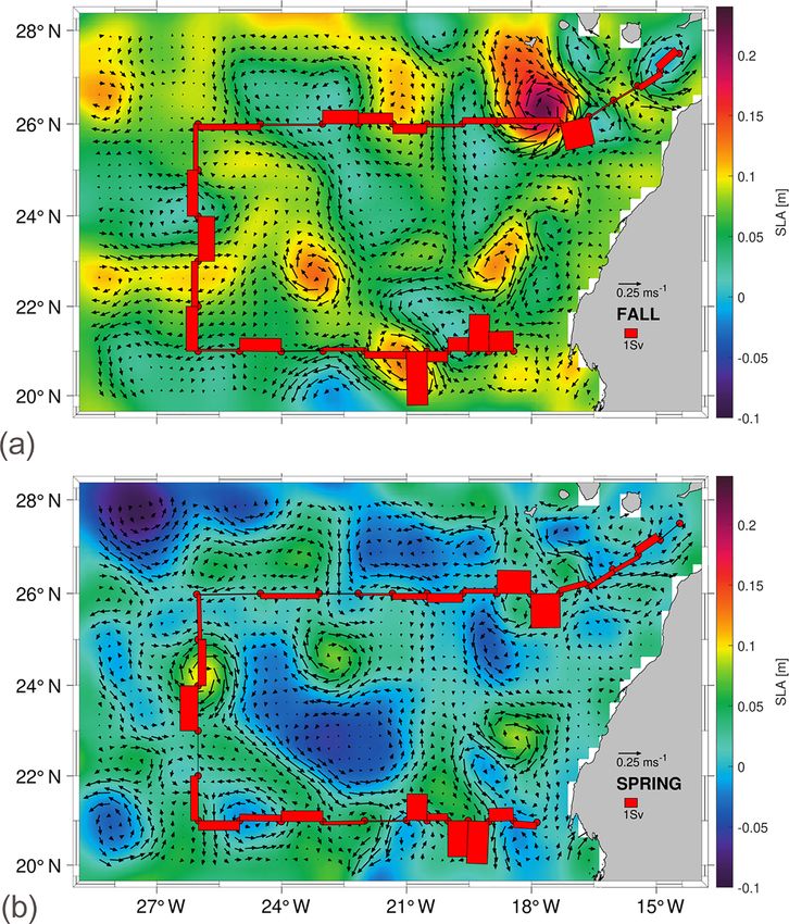
www.ocean-sci.net/16/483/2020/ Ocean Sci., 16, 483–511, 2020496 N. Burgoa et al.: Mass, nutrients and DOC lateral transports off NW Africa Figure 9. Reference-level velocity at 27.962 kg m−3 and its standard deviation estimated by the inverse model during fall (a) and spring (b). The direction chosen for the representation is the same as in Fig. 2. The signs of the velocity are according to the geographical criterion; i.e., the velocities are positive–negative toward north–south in the northern and southern transects, and they are positive–negative toward east–west in the western transect. are higher than those observed in spring at similar loca- axis has the same direction as the rest of the vertical sec- tions (Fig. 7). Furthermore, high concentrations of DOC in tions, and the three transects are separated by two vertical fall at CW levels are recorded in the same area where the dashed grey lines. The Sverdrup (Sv) is used here as equiva- deep anticyclonic eddy is located, between stations 8 and 18 lent to 109 kg s−1 . The positive–negative transport values in- (Fig. 8). In spring, mesoscale structures in the vertical sec- dicate outward–inward transports from–to the box. The accu- tions of INs and DOC at CW levels are less intense than in mulated mass transports show a significant horizontal spatial fall (Fig. 10). Nonetheless, DOC concentrations below the variability, especially marked in the southern transect in ac- two anticyclonic structures at CW levels in spring are higher cordance with the geostrophic velocity distribution (Fig. 10). than in their surroundings. The presence of significant mesoscale structures might be The accumulated geostrophic mass transport is integrated one of the sources of the total imbalances in the accumulated to group the variability at different levels, with the first shal- mass transport. In fall, the total imbalance is −1.43 Sv, and lowest layer for SW, the next four layers for CW, then two in spring it is 3.55 Sv (Table 4). layers for IW and the deepest two layers for DW (Fig. 12). On the other hand, the geostrophic mass transport can be The total accumulated geostrophic mass transport, integrated integrated per layer and transect together with the total im- for all the nine layers, is also represented. The horizontal balance inside the box and the total mass transport uncer- Ocean Sci., 16, 483–511, 2020 www.ocean-sci.net/16/483/2020/
N. Burgoa et al.: Mass, nutrients and DOC lateral transports off NW Africa                                                              497

Figure 10. Sections of the absolute geostrophic velocity with respect to γn during fall (a) and spring (b). The horizontal axis has the same
direction as Fig. 2, and the criterion of the velocity signs is as in Fig. 9. The depths 150, 672–700 and 1294–1305 m are highlighted by grey
isolines as in the γn sections in Figs. 4 and 5.

tainty per layer (the black line and horizontal black bars in            is reversed to a net outward flow in spring at the southern
Fig. 13). Table 4 compiles these transports integrated for               transect (Fig. 13).
the different water levels, which are also represented geo-                 The position of the CVFZ in both seasons could partly ex-
graphically in Fig. 14. More than 65 % of the mass trans-                plain the seasonal variability in the mass transports at central
port is given at SW and CW levels (Table 4). In fall, these              levels (Fig. 15). In fall, the CVFZ is located further from
water masses mostly move into the box across the north-                  the African coast, so SACW is present at almost all stations
ern and southern transects, with transports of −5.61 ± 1.86              of the south transect. This location of the CVFZ prevents a
and −4.35 ± 1.48 Sv, respectively; the mass leaves the box               latitudinal mass transport from north to south. However, in
by flowing westward with a value of 5.96 ± 1.75 Sv. In                   spring the CVFZ is closer to the African slope, allowing for
spring, water masses also move into the box mostly through               an important mass transport from north to south.
the northern transect with −6.69 ± 1.63 Sv, but they leave                  Between 5 % and 30 % of the mass transport is given in
along the western and southern transects with transports of              intermediate levels (Table 4). In fall, the intermediate wa-
4.05 ± 1.75 and 5.20 ± 1.55 Sv, respectively. It is remarkable           ter transport is directed northward in the southern transect
how the inward transport in fall across the southern transect            with −1.93 ± 1.69 Sv, and it leaves the box with 1.94 ± 1.85

www.ocean-sci.net/16/483/2020/                                                                            Ocean Sci., 16, 483–511, 2020
498                                               N. Burgoa et al.: Mass, nutrients and DOC lateral transports off NW Africa

Figure 11. Average derived geostrophic velocity and SLA during fall (a) in the course of the fist cruise and spring (b) in the course of the
second cruise, extracted from AVISO+. The red bars represent the mass transports in the shallowest layer as estimated by the inverse model.

and 0.48 ± 1.71 Sv across the northern and western tran-                5.2    Nutrient and DOC transports
sects, respectively. During spring, this transport weakens and
changes its direction in the northern and southern transects            DOC and IN transports are obtained by multiplying their
with transports of −0.48 ± 1.65 and 0.39 ± 1.73 Sv, respec-             concentration by mass transports. DOC, INs and geostrophic
tively, increasing its westward transport to 1.21 ± 1.68 Sv.            velocities are obtained at different locations, so they need to
   The mass transport in deepwater layers barely exceeds 3 %            be interpolated to a common grid. In the case of DOC, the
(Table 4). An exception is the 8 % given in the northern                velocities are horizontally interpolated to the locations where
transect during fall when the estimated transport is 0.73 ±             the concentrations of DOC are taken, and, in a second step,
1.71 Sv. During both cruises the transport at deep levels was           the concentrations of DOC are linearly interpolated to the
nearly balanced.                                                        depths of the geostrophic velocities. On the other hand, the
                                                                        in situ measurements of INs are scarce at IW and DW where
                                                                        their concentrations become higher. Therefore, instead of us-
                                                                        ing the observational data, the average outputs of GLORYS-
                                                                        BIO are used to estimate the IN transports. SiO2 , NO3 and

Ocean Sci., 16, 483–511, 2020                                                                         www.ocean-sci.net/16/483/2020/
N. Burgoa et al.: Mass, nutrients and DOC lateral transports off NW Africa 499 Figure 12. Accumulated mass transport along the fall (a) and spring (b) cruises at the surface waters (SW, in red and dashed line), central waters (CW, in red line), intermediate waters (IW, in green line) and deep waters (DW, in blue line). The accumulated mass transport integrated for all nine layers is also represented. The horizontal axis has the same direction as Fig. 2. Negative–positive values of transports along the three transects indicate inward–outward transports in the box delimited by the three transects and the African coast. PO4 mean concentrations are interpolated to the grid nodes ports. The DOC transport estimates per layer and transect are for which the geostrophic velocities are estimated by the in- also shown in Fig. 17 and summarized per water level and verse model. transect with their relative error (calculated as in the IN trans- DOC transports are obtained by subtracting a refractory ports) in Table 8. In order to be able to compare our transport concentration of 40 µmol L−1 from the measured DOC (e.g., values of INs and DOC with those reported by other authors, Santana-Falcón et al., 2017). This is done because the refrac- equivalent units are employed for IN (kmol s−1 ) and DOC tory fraction renewal is thousands of years, a period much transports (×108 mol C d−1 ). longer than the time required in the processes we are focused INs enter the domain both from the north and south at on (Hansell, 2002). On the other hand, it should be empha- CW in fall. At the northern transect the transports are rel- sized that DOC transports may be underestimated due to the atively low, while at the southern one transports double the scarcity of available measurements. amount coming from north, with −0.41±0.11, −0.78±0.21 The IN transport values are presented in the text always and −0.05 ± 0.01 kmol s−1 . In spring, instead, the IN trans- ordered as SiO2 , NO3 and PO4 (Figs. 16 and 17). Tables 5, 6 ports change their direction in the southern transect and only and 7 summarize those transports integrated per water level enter from the north, with values double those during fall, and transect. The errors are relative to the mass transport er- −0.40 ± 0.09, −0.90 ± 0.21, −0.06 ± 0.01 kmol s−1 . On the rors and are calculated as the standard deviations of IN trans- other hand, IN transports at CW layers are overall westward www.ocean-sci.net/16/483/2020/ Ocean Sci., 16, 483–511, 2020
500                                                N. Burgoa et al.: Mass, nutrients and DOC lateral transports off NW Africa

Table 4. Mass transports with their errors (Sv) for SW, CW, IW and DW across the north, west and south transects for both seasons. Positive–
negative values indicate outward–inward transports. The last row is the integrated transport for the entire water column in each transect, while
the fourth column summarizes the imbalances in mass transport for both seasons.

                          Water levels    Season             North           West             South       Imbalance
                                          Fall       −2.67 ± 0.60     2.46 ± 0.66     −0.50 ± 0.45     −0.71 ± 1.00
                          SW
                                          Spring     −1.80 ± 0.49     1.09 ± 0.69      2.40 ± 0.53      1.70 ± 0.99
                                          Fall       −2.94 ± 1.26     3.50 ± 1.09     −3.85 ± 1.03     −3.29 ± 1.95
                          CW
                                          Spring     −4.89 ± 1.14     2.96 ± 1.06      2.80 ± 1.02      0.87 ± 1.86
                                          Fall        1.94 ± 1.85     0.48 ± 1.71     −1.93 ± 1.69       0.49 ± 3.03
                          IW
                                          Spring     −0.48 ± 1.65     1.21 ± 1.68      0.39 ± 1.73        1.1 ± 2.92
                                          Fall        0.73 ± 1.71     0.32 ± 1.56       0.19 ± 1.37      1.24 ± 2.69
                          DW
                                          Spring     −0.04 ± 1.54     0.09 ± 1.53       0.00 ± 1.42      0.05 ± 2.59
                                          Fall       −2.59 ± 2.88     6.99 ± 2.64     −5.82 ± 2.45     −1.43 ± 4.61
                          Total
                                          Spring     −7.24 ± 2.57     5.27 ± 2.60      5.53 ± 2.52      3.55 ± 4.44

Table 5. SiO2 transports and their errors (kmol s−1 ) for CW, IW and DW for the north, west and south transects. Positive–negative values
indicate outward–inward transports. The last row is the integrated transport in the entire water column in each transect, and the last column
represents the net transport for this variable inside the box.

                         Water levels    Season             North             West             South       Imbalance
                                         Fall       −0.06 ± 0.01       0.06 ± 0.02       0.02 ± 0.02      0.02 ± 0.02
                         SW
                                         Spring     −0.06 ± 0.02       0.04 ± 0.02       0.06 ± 0.01      0.04 ± 0.02
                                         Fall       −0.14 ± 0.06       0.21 ± 0.06     −0.41 ± 0.11     −0.34 ± 0.20
                         CW
                                         Spring     −0.40 ± 0.09       0.45 ± 0.16      0.23 ± 0.08      0.28 ± 0.61
                                         Fall        0.23 ± 0.22     −0.13 ± 0.45      −0.27 ± 0.24     −0.17 ± 1.07
                         IW
                                         Spring     −0.04 ± 0.15      0.19 ± 0.27       0.12 ± 0.55      0.28 ± 0.72
                                         Fall        0.13 ± 0.31     −0.11 ± 0.52      −0.14 ± 1.00     −0.12 ± 0.25
                         DW
                                         Spring     −0.01 ± 0.51      0.06 ± 1.15      0.08 ± 13.38      0.13 ± 6.79
                                         Fall        0.16 ± 0.17       0.03 ± 0.01     −0.80 ± 0.34     −0.61 ± 1.97
                         Total
                                         Spring     −0.51 ± 0.18       0.75 ± 0.37      0.49 ± 0.22      0.73 ± 0.91

with low values in fall, while in spring IN transports are                values due to the low velocities at these depths, despite their
southward and westward.                                                   high nutrient concentrations (Figs. 16 and 17). Furthermore,
   At IW levels, during fall the IN transports are inward                 the relative error in these layers is always larger than the IN
through the southern transect, with −0.27 ± 0.24, −0.36 ±                 transport values.
0.32 and −0.02 ± 0.02 kmol s−1 , and to a lesser extent                      In spring, DOC transports at SW and CW levels are the
through the western transect. Outward transports are ob-                  same order of magnitude and 1 order of magnitude higher
served through the northern transect with 0.23±0.22, 0.30±                than those at IW levels. In turn, these transports at IW levels
0.28 and 0.02 ± 0.02 kmol s−1 . In spring, the INs enter                  are 1 order of magnitude higher than those at DW levels dur-
weakly through the northern transect and leave the box,                   ing this season. In contrast, during fall at the northern tran-
crossing the western and southern transects with significant              sect DOC transports have the same magnitude in SW, CW
values of 0.19 ± 0.27 and 0.12 ± 0.55 kmol s−1 for SiO2 ,                 and IW, and they are 1 order of magnitude smaller than those
0.25±0.35 and 0.17±0.75 kmol s−1 for NO3 , and 0.02±0.02                  at CW levels during spring (Table 8). In this season, DOC
and 0.01 ± 0.05 kmol s−1 for PO4 . In summary, while in fall              transports at SW and CW in the western transect have un-
the main IN transports are in the south to north direction, in            realistically small values likely related to the low number of
spring they are mainly southwestward like the mass transport              measurements made in this transect during fall. DOC trans-
behavior at these levels during this season (Table 4).                    ports through the northern transect could also be somewhat
   Finally, at DW during both seasons, the net transports of              underestimated for the same reason. However, at the southern
the three nutrients are similar to those at IW but with smaller

Ocean Sci., 16, 483–511, 2020                                                                            www.ocean-sci.net/16/483/2020/
N. Burgoa et al.: Mass, nutrients and DOC lateral transports off NW Africa 501
Table 6. NO3 transports and their errors (kmol s−1 ) for CW, IW and DW for the north, west and south transects. Positive–negative values
indicate outward–inward transports. The last row is the integrated transport in the entire water column in each transect, and the last column
represents the net transport of this variable inside the box.
Water levels Season North West South Imbalance
Fall −0.05 ± 0.01 0.13 ± 0.04 0.17 ± 0.15 0.25 ± 0.35
SW
Spring −0.03 ± 0.01 0.12 ± 0.07 0.07 ± 0.02 0.16 ± 0.09
Fall −0.36 ± 0.15 0.47 ± 0.15 −0.78 ± 0.21 −0.67 ± 0.40
CW
Spring −0.90 ± 0.21 0.91 ± 0.33 0.56 ± 0.20 0.57 ± 1.22
Fall 0.30 ± 0.28 −0.16 ± 0.57 −0.36 ± 0.32 −0.23 ± 1.39
IW
Spring −0.06 ± 0.20 0.25 ± 0.35 0.17 ± 0.75 0.36 ± 0.94
Fall 0.13 ± 0.30 −0.10 ± 0.48 −0.13 ± 0.91 −0.10 ± 0.21
DW
Spring −0.01 ± 0.52 0.06 ± 1.05 0.08 ± 12.63 0.12 ± 6.26
Fall 0.02 ± 0.02 0.35 ± 0.13 −1.11 ± 0.47 −0.74 ± 2.40
Total
Spring −1.01 ± 0.36 1.34 ± 0.66 0.88 ± 0.40 1.21 ± 1.51
Table 7. PO4 transports and their errors (kmol s−1 ) for CW, IW and DW for the north, west and south transects. Positive–negative values
indicate outward–inward transports. The last row is the integrated transport in the entire water column in each transect, and the last column
represents the net transport of this variable inside the box.
Water levels Season North West South Imbalance
Fall −0.00 ± 0.00 0.01 ± 0.00 0.01 ± 0.01 0.02 ± 0.02
SW
Spring −0.00 ± 0.00 0.01 ± 0.01 0.01 ± 0.00 0.01 ± 0.01
Fall −0.02 ± 0.01 0.03 ± 0.01 −0.05 ± 0.01 −0.04 ± 0.02
CW
Spring −0.06 ± 0.01 0.06 ± 0.02 0.04 ± 0.01 0.04 ± 0.08
Fall 0.02 ± 0.02 −0.01 ± 0.04 −0.02 ± 0.02 −0.01 ± 0.09
IW
Spring −0.00 ± 0.01 0.02 ± 0.02 0.01 ± 0.05 0.02 ± 0.06
Fall 0.01 ± 0.02 −0.01 ± 0.03 −0.01 ± 0.06 −0.01 ± 0.01
DW
Spring −0.00 ± 0.04 0.00 ± 0.07 0.01 ± 0.85 0.01 ± 0.42
Fall 0.00 ± 0.00 0.02 ± 0.01 −0.07 ± 0.03 −0.05 ± 0.15
Total
Spring −0.06 ± 0.02 0.08 ± 0.04 0.06 ± 0.03 0.08 ± 0.10
transect during fall, the result is of the same order of magni- ing the box is larger than those leaving the box, with the ex-
tude as in spring. ception of the shallowest level at which the INs leave the box
In spring, DOC transports behave in a similar way in (Tables 5, 6 and 7 and Figs. 16 and 17). On the other hand, the
the entire water column. At SW and CW levels, −2.33 ± net DOC transports are outward for SW, CW and IW levels
0.57 × 10⁸ mol C d−1 enters through the northern transect, with 0.10±0.13×10⁸ mol C d−1 at SW levels, 1.34±0.80×
0.89 ± 0.25 × 10⁸ mol C d−1 of which leaves the box through 108 mol C d−1 at CW levels and 0.12 ± 0.72 × 10⁸ mol C d−1
the southern transect, approximately half of it through the at IW (Table 8 and Fig. 17).
western transect. During fall, there is an important outward In contrast, during spring a net outward transport is ob-
DOC transport at SW, CW and IW levels, especially south- tained for the three INs with 0.28 ± 0.61, 0.57 ± 1.22 and
ward through the southern transect at SW and CW levels, 0.04 ± 0.08 kmol s−1 at CW, 0.28 ± 0.72, 0.36 ± 0.94 and
with a total of 1.48 ± 0.66 × 10⁸ mol C d−1 (Table 8). 0.02 ± 0.06 kmol s−1 at IW, and 0.13 ± 6.79, 0.12 ± 6.26
Two opposite trends can be observed when both cruises and 0.01 ± 0.42 kmol s−1 at DW (Tables 5, 6 and 7, and
are compared. In fall the IN net transports are −0.34 ± Figs. 16 and 17). The DOC net transports are inward
0.20, −0.67 ± 0.40 and −0.04 ± 0.02 kmol s−1 at CW lev- with −0.14 ± 0.08 × 10⁸ mol C d−1 at SW level; −0.80 ±
els; −0.17 ± 1.07, −0.23 ± 1.39 and −0.01 ± 0.09 kmol s−1 1.72 × 10⁸ mol C d−1 at CW levels; and −0.01 ± 0.02 ×
at IW levels; and −0.12 ± 0.25, −0.10 ± 0.21 and −0.01 ± 108 mol C d−1 at IW levels (Table 8 and Fig. 17).
0.01 kmol s−1 at DW levels. The amount of nutrients enter-
www.ocean-sci.net/16/483/2020/ Ocean Sci., 16, 483–511, 2020You can also read