VESPA-22: a ground-based microwave spectrometer for long-term measurements of polar stratospheric water vapor - Atmos. Meas. Tech
←
→
Page content transcription
If your browser does not render page correctly, please read the page content below
Atmos. Meas. Tech., 11, 1099–1117, 2018
https://doi.org/10.5194/amt-11-1099-2018
© Author(s) 2018. This work is distributed under
the Creative Commons Attribution 4.0 License.

VESPA-22: a ground-based microwave spectrometer for long-term
measurements of polar stratospheric water vapor
Gabriele Mevi1,2 , Giovanni Muscari1 , Pietro Paolo Bertagnolio1,a , Irene Fiorucci1,b , and Giandomenico Pace3
1 IstitutoNazionale di Geofisica e Vulcanologia, Rome, 00143, Italy
2 Mathematics    and Physics Department, Roma Tre University, Rome, 00146, Italy
3 ENEA, Laboratory for Observations and Analyses of Earth and Climate, Rome, 00123, Italy
a now at: AECOM, Croydon, CRO 2AP, UK
b now at: Istituto Paritario Vincenzo Pallotti, Rome, 00122, Italy

Correspondence: Gabriele Mevi (gabriele.mevi@ingv.it)

Received: 26 July 2017 – Discussion started: 14 August 2017
Revised: 6 December 2017 – Accepted: 11 January 2018 – Published: 23 February 2018

Abstract. The new ground-based 22 GHz spectrometer,              tained from 24 h averaged spectra and are compared with
VESPA-22 (water Vapor Emission Spectrometer for Polar            version 4.2 of concurrent Aura/Microwave Limb Sounder
Atmosphere at 22 GHz) measures the 22.23 GHz water va-           (MLS) water vapor vertical profiles. In the sensitivity range
por emission line with a bandwidth of 500 MHz and a fre-         of VESPA-22 retrievals, the intercomparison from July 2016
quency resolution of 31 kHz. The integration time for a mea-     to July 2017 between VESPA-22 dataset and Aura/MLS
surement ranges from 6 to 24 h, depending on season and          dataset convolved with VESPA-22 averaging kernels shows
weather conditions. Water vapor spectra are collected using      an average difference within 1.4 % up to 60 km altitude and
the beam-switching technique. VESPA-22 is designed to op-        increasing to about 6 % (0.2 ppmv) at 72 km.
erate automatically with little maintenance; it employs an un-
cooled front-end characterized by a receiver temperature of
about 180 K and its quasi-optical system presents a full width
at half maximum of 3.5◦ . Every 30 min VESPA-22 measures         1   Introduction
also the sky opacity using the tipping curve technique. The
instrument calibration is performed automatically by a noise     The polar atmosphere is a very complex system in which wa-
diode; the emission temperature of this element is estimated     ter vapor plays an important role. Water vapor has a major
twice an hour by observing alternatively a black body at am-     impact on the radiative balance affecting both infrared ra-
bient temperature and the sky at an elevation of 60◦ . The       diation by greenhouse effect and visible radiation by clouds
retrieved profiles obtained inverting 24 h integration spectra   coverage. The importance of water vapor in the Arctic region
present a sensitivity larger than 0.8 from about 25 to 75 km     is enhanced by the so-called Arctic amplification effect (Ser-
of altitude during winter and from about 30 to 65 km dur-        reze and Francis, 2006), a positive feedback that links the
ing summer, a vertical resolution from about 12 to 23 km         quantity of water vapor in the atmosphere, the presence of
(depending on altitude), and an overall 1σ uncertainty lower     clouds, the ice coverage, and the surface temperature. Addi-
than 7 % up to 60 km altitude and rapidly increasing to 20 %     tionally, about 10 % of the surface warming measured during
at 75 km.                                                        the last two decades can be ascribed to stratospheric water
   In July 2016, VESPA-22 was installed at the Thule High        vapor, as shown by Solomon et al. (2010).
Arctic Atmospheric Observatory located at Thule Air Base            The characterization of the water vapor profile, particu-
(76.5◦ N, 68.8◦ W), Greenland, and it has been operating al-     larly in the stratosphere and mesosphere, is important to un-
most continuously since then. The VESPA-22 water vapor           derstand many chemical processes. Polar water vapor is di-
mixing ratio vertical profiles discussed in this work are ob-    rectly involved in the ozone chemistry as the main source of
                                                                 the OH radical in reactions that cause the ozone destruction

Published by Copernicus Publications on behalf of the European Geosciences Union.
1100                                                                                                  G. Mevi et al.: VESPA-22

(Solomon, 1999). It is also related to the formation of polar       nolio et al., 2012). The quasi-optical system, consisting of an
stratospheric clouds (PSCs) that grant the catalytic surfaces       antenna and parabolic mirror, has a full width at half maxi-
on which heterogeneous reactions take place.                        mum (FWHM) θ3 dB = 3.5◦ (Bertagnolio et al., 2012). This
   The main sources of middle atmosphere water vapor are            high directivity of the system allows the observation at an-
transport through the tropical tropopause and methane ox-           gles as low as 12◦ above the horizon, therefore maximizing
idation, whereas the main sink is photolysis in the Lyman           the number of emitting molecules and the signal-to-noise ra-
band. In the middle atmosphere, the lifetime of water vapor         tio of the measurement.
varies from several days to weeks, making it a valuable tracer         A first uncooled low noise amplification stage amplifies
for the investigation of dynamical processes that characterize      the incoming signal with a gain of 35 dB. Two noise diodes
the polar regions especially during winter and spring.              manufactured by Noisecom are inserted in the radio fre-
   The processes that lead to long-term variations in strato-       quency (RF) chain after the choke antenna by means of two
spheric and mesospheric water vapor are not completely un-          20 dB broadwall direction couplers. These two diodes pro-
derstood. Positive trends were observed during the 1980–            duce a signal which is measured to average at about 119 and
2000 period (Nedoluha et al., 1999; Rosenlof et al., 2001)          78 K and are used to calibrate the sky signal observed by
and Oltmans et al. (2000) suggested that only one-half of           VESPA-22, as described in Sect. 3.3.
these changes are related to anthropogenic activities.                 After the 20 dB couplers the signal is amplified and down-
   The comprehension of the change in climate that affects          converted to lower frequencies and eventually sampled at
the Arctic and the peculiar characteristics of this region’s at-    1 Gs s−1 by a fast Fourier transform spectrometer (FFTS; Ac-
mosphere calls for long-term measurements. For this task,           quiris AC240/Agilent U1080 A-001) with 16 384 channels,
ground-based microwave remote sensing is a powerful tool            resulting in a spectral resolution of 31 kHz for a total band-
to measure water vapor profiles and total amount of precip-         width of 500 MHz.
itable water vapor (PWV).                                              During measurements, the antenna is moved back and
   In this paper, VESPA-22 (water Vapor Emission Spec-              forth to change its distance from the mirror by λ/4 =
trometer for Polar Atmosphere at 22 GHz), a microwave               3.34 mm in order to avoid multiple internal reflections of the
spectrometer developed at the INGV (Istituto Nazionale di           signal which would cause the formation of standing waves
Geofisica e Vulcanologia) is presented. In July 2016, dur-          affecting the observed spectrum. One full spectrum is ob-
ing the Study of the water VApor in the polar AtmosPhere            tained by averaging together two 6 min spectra collected with
(SVAAP) measurements campaign, a key part of a research             the antenna positioned at these two different distances from
effort devoted to the study of the impact of water vapor and        the mirror. Once a day, two photodiodes are employed to
clouds on the radiation budget at the ground, VESPA-22              check and reset the correct distance between the antenna and
was installed at the Thule High Arctic Atmospheric Observa-         the mirror.
tory (THAAO) located at Thule Air Base (76.5◦ N, 68.8◦ W),             VESPA-22 is installed indoors to protect it from the strong
Greenland. The instrument general features, the measure-            winds and storms which can occur during most of the year.
ment physics and technique, a comparison between VESPA-             The indoor installation prevents the deposition on the quasi-
22 and the Aura/Microwave Limb Sounder (MLS) (Waters                optical system of snow in winter and dust in summer, as well
et al., 2006) version 4.2 datasets are discussed in this work.      as the condensation of water droplets, therefore improving
                                                                    the durability of the equipment. Additionally, the parabolic
                                                                    mirror and its driving motor are not exposed to strong winds,
2   Instrumental setup                                              and VESPA-22 is therefore characterized by a pointing offset
                                                                    that is very stable with time. The instrument is located in
VESPA-22 collects the microwave radiation emitted by the            a small wooden annex (Fig. 2) to the main observatory in
water vapor transition at 22.235 GHz with a spectral resolu-        order to minimize the presence of metal surfaces which could
tion of 31 kHz and a bandwidth of 500 MHz. From the spec-           also yield standing waves in the observed spectrum.
tral measurements water vapor profiles can be retrieved with           The spectrometer observes the sky through two 5 cm thick
a temporal resolution of 1–4 profiles a day, depending on sea-      Plastazote LD15 windows, one covering the observation at
son and weather conditions. The instrument also measures            angles from 10 to 60◦ above the horizon and a smaller one
the sky opacity in few minutes by performing a scan of the          covering the zenith direction (see Figs. 1 and 2). This mate-
sky at various angles called tipping curve.                         rial was tested in the laboratory and proved to have a neg-
   In Fig. 1, a photo and the layout of the spectrometer are        ligible absorption in the microwave region of interest. Fur-
displayed. VESPA-22 collects the sky signal coming from             thermore, the windows are not perpendicular to the antenna
different elevation angles using a parabolic mirror. The signal     beam in order to minimize any potential formation of stand-
is reflected by the mirror to a Gaussian choked horn antenna        ing waves. The opacity of the LD15 window sheets was esti-
(Teniente et al., 2002). This antenna has a far field directivity   mated during VESPA-22 installation and it was measured to
of 23.5 dB with a pattern that can be approximated at 99.85 %       be less than 0.0005 Np. Three powerful fans are employed to
to a Gaussian beam with a beam waist of 22.4 mm (Bertag-            blow off the snow from the observing windows, preventing

Atmos. Meas. Tech., 11, 1099–1117, 2018                                               www.atmos-meas-tech.net/11/1099/2018/
G. Mevi et al.: VESPA-22                                                                                                            1101

Figure 1. A photo of VESPA-22 installed at the THAAO, Thule Air Base, Greenland (left), and the layout of the instrument (right).

                                                                       will be explained in Sect. 3.2. The zenith is observed through
                                                                       a white Delrin® acetal homopolymer resin sheet, hereafter
                                                                       simply delrin (see Fig. 1), which adds a grey-body emission
                                                                       to the reference beam; this sheet is set at Brewster’s angle
                                                                       with respect to the incident beam in order to minimize re-
                                                                       flections and the formation of standing waves.
                                                                          During an hour of standard instrument operations, about
                                                                       3 min is dedicated to tipping curves (see Sect. 3.4) used to
                                                                       measure tropospheric opacity, about 35 min is dedicated to
                                                                       measure the emissions from the signal and reference beams,
                                                                       and the rest of the hour is dedicated to instrumental opera-
                                                                       tions, such as the rotation of the parabolic mirror or the in-
                                                                       strument calibration by means of the noise diodes.

                                                                       3   Measurement technique

                                                                       VESPA-22 collects the 22.235 GHz radiation emitted by wa-
                                                                       ter vapor molecules. At this frequency, the Rayleigh–Jeans
                                                                       approximation for the Plank’s law can be used and the radi-
Figure 2. A photo of the exterior of the wooden annex hosting          ation intensity can be expressed in terms of brightness tem-
VESPA-22. The observing window of the signal beam is visible on        perature. The line shape of the emission from a stratospheric
the side of the annex.                                                 altitude z is mainly a function of atmospheric pressure:

                                                                                       T0 n

                                                                       1ν ∝ P (z)             ,                                  (1)
                                                                                      T (z)
deposition or ice formation on the external side of the win-
dows. VESPA-22 compares the sky emission from the zenith               where 1ν is the line width, n < 1 is a constant coefficient
direction (also called reference direction) to the sky emis-           and T0 = 300 K (see Table 3, Sect. 4.1, for the spectroscopic
sion from an angle close to the horizon (also called signal di-        values used for VESPA-22 retrievals). Using this dependence
rection) in order to perform a stratospheric measurement, as           and knowing the pressure and temperature atmospheric pro-

www.atmos-meas-tech.net/11/1099/2018/                                                    Atmos. Meas. Tech., 11, 1099–1117, 2018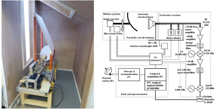
1102                                                                                                   G. Mevi et al.: VESPA-22

files, the measured spectrum can be inverted using the re-         right side is the extra-atmospheric emission, the second term
verse problem theory to obtain the vertical water vapor mix-       is the solution of the radiative transfer equation for an isother-
ing ratio profile. In the mesosphere, the Doppler broadening       mal domain where the tropospheric emission is indicated
overcomes the pressure broadening of Eq. (1) determining           with Ttrop and represents the mean tropospheric temperature
an upper limit to the altitude range in which the water va-        weighted with the water vapor concentration. The third term
por profile can be retrieved. In the lower stratosphere, the       on the right is the emission coming from the stratosphere and
broadening makes the line width comparable to the VESPA-           mesosphere, T (ν), proportional to the air mass factor µ and
22 spectral bandpass, therefore setting a lower altitude limit     attenuated in the troposphere by a factor e−µτ . The air mass
for the deconvolved profile.                                       factor at the elevation angle θ is computed according to the
                                                                   formula presented in the work of de Zafra (1995).
3.1    Atmospheric opacity
                                                                   3.2   Beam-switching technique
The majority of the incoming radiation measured by VESPA-
22 comes from the troposphere. The tropospheric emission           The technique that VESPA-22 employs to measure the strato-
needs to be filtered in order to study the stratospheric signal.   spheric signal is called the beam-switching technique or
In order to simplify the radiative transfer equation, the fol-     Dicke switching technique (e.g., Parrish et al., 1988). The
lowing approximations can be adopted (e.g., Nedoluha et al.,       instrument compares the emission coming from an observa-
1995).                                                             tion angle θ (signal beam) with a reference signal with the
                                                                   same mean power over the passband. The observation an-
  – The troposphere is represented as an isothermal layer          gle depends on the atmospheric opacity and for VESPA-22
    absorbing the signal to be measured. The first kilo-           it varies from 12 to 25◦ above the horizon. The reference
    meters of the atmosphere produce the greatest part of          signal used by VESPA-22 is the sky emission at the zenith
    this layer emission which has a line width larger than         (reference beam). In clear-sky conditions, the emission at the
    VESPA-22 bandwidth. This contribution is treated as an         zenith is smaller than the emission at a much larger zenith
    emission constant in frequency.                                angle. Therefore, in order to ensure that the reference beam
                                                                   has the same mean power of the signal beam, a thin sheet of
  – The contribution of the stratospheric water vapor ab-
                                                                   delrin is inserted in the reference beam. The delrin sheet acts
    sorption to the opacity τ is small. This approxima-
                                                                   as a grey body so that
    tion was tested by calculating the atmospheric opacity
    by means of the radiative transfer simulation software         TR (ν) = T0 e−τ −τd + Ttrop 1 − e−τ e−τd

    ARTS (Eriksson et al., 2011) and using water vapor ver-
                                                                      + T (ν) e−τ −τd + Td 1 − e−τd ,

                                                                                                                               (3)
    tical profiles with and without their stratospheric com-
    ponent. At the frequency of maximum absorption, the            where TR is the radiation observed by VESPA-22 coming
    contribution of the stratospheric profile to the overall       from the zenith, partially absorbed by the delrin sheet, Td is
    atmospheric opacity is between 2 and 5 % depending             the physical temperature of the sheet and τd its mean opac-
    on the season. When averaged over the VESPA-22 fre-            ity value over the spectral passband. In this equation, the air
    quency range, the difference between the opacity calcu-        mass factor µ is equal to 1.
    lated using a full water vapor vertical profile and a pro-        During data-taking operations, VESPA-22 alternates ref-
    file with no water vapor above the tropopause is be-           erence and signal observations. The instrument constantly
    tween 0.4 and 1.5 %.                                           checks if the two beams have the same mean power and con-
                                                                   tinuously changes the signal angle to minimize the difference
  – The opacity τν can be substituted by its mean value τ .
                                                                   between them. When the two beams have the same intensity,
    The maximum difference between τν and its mean value
                                                                   the frequency independent terms of Eqs. (3) and (2) can be
    τ is between 1.6 and 3.6 % depending on season.
                                                                   equated, obtaining
  – The only signal coming from outside the atmosphere,
                                                                   T0 e−τ −τd + Ttrop 1 − e−τ e−τd + Td 1 − e−τd

    T0 , is the cosmic background radiation with a constant
                                                                       ≈ T0 e−µτ + Ttrop 1 − e−µτ ,

    brightness temperature of 2.73 K.                                                                                          (4)

  With these approximations the radiative transfer equation        where the stratospheric contribution to the mean beam inten-
describing the radiation received at the ground from an ele-       sity (about 1 %) is neglected (de Zafra, 1995).
vation angle θ can be written as                                      The stratospheric signal T (ν) is obtained by subtracting
                                                                   reference from signal. Using Eqs. (2), (3) and (4) it is possi-
TS (ν) = T0 e−µτ + Ttrop 1 − e−µτ + µT (ν) e−µτ .

                                                         (2)       ble to write

                                                                   TS (ν) − TR (ν) ≈ T (ν) µe−µτ − e−τ −τd

The left term is the radiation received by the spectrometer                                                                    (5)
when pointing at the elevation angle θ . The first term on the     and

Atmos. Meas. Tech., 11, 1099–1117, 2018                                               www.atmos-meas-tech.net/11/1099/2018/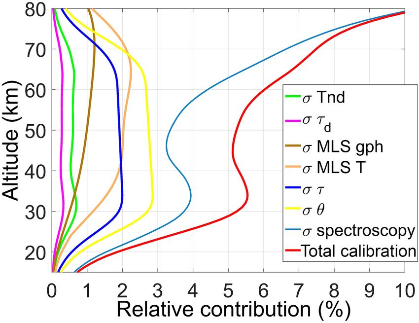
G. Mevi et al.: VESPA-22                                                                                                        1103

          TS (ν) − TR (ν)
T (ν) =                   .                                (6)    Table 1. Mean values and SDs (standard deviations) of the mea-
          µe−µτ − e−τ −τd                                         sured opacity for the two used delrin sheets during different sea-
                                                                  sons.
   Three delrin sheets with different thicknesses (3, 5, and
9 mm) and opacities can be employed, depending on the sea-          Thickness         July 2016      November 2016    February 2017
son, in order to maintain the signal angle between 12 and           9 mm         0.159 ± 0.004        0.128 ± 0.003   0.123 ± 0.003
25◦ above the horizon. Spectra collected are smoothed us-           5 mm         0.088 ± 0.001        0.072 ± 0.001   0.070 ± 0.001
ing a 50-channel moving average. This smoothing process is,
however, not performed in a 6 MHz interval centered around
the emission line to maintain the maximum frequency reso-         the incoming signal to the FFTS, is measured approximately
lution near the line peak.                                        every 15 min and it is subtracted to each signal and reference
   In order to estimate τd , the mean opacity value of delrin     15 min integration spectra which are eventually saved on the
over the spectral passband, during normal data-taking oper-       control and acquisition PC (see Fig. 1). Using Eq. (8), Eq. (6)
ations the signal angle is locked to its balanced position and    can be written as
the delrin sheet is removed from the reference beam. τd can                   1 VS (ν) − VR (ν)
then be calculated using                                          T (ν) =                         .                               (9)
                                                                            α (ν) µe−µτ − e−τ −τd
                        !
              Td − T S                                            VESPA-22 measures the gain parameter α by means of the
τd = − ln                  ,                                (7)
            Td − T Rnod                                           noise diode. As mentioned before, VESPA-22 has two dif-
                                                                  ferent noise diodes, one used to perform regular calibrations
where T Rnod is the mean intensity of the reference beam with-    and the second inserted to ensure the stability over time of the
out the sheet and T S is the mean value of the signal beam.       first one, as described by Gomez et al. (2012). During regu-
The brightness temperatures T S and T Rnod are calculated us-     lar measurements, the calibration noise diode is switched on
ing parameters obtained by means of a calibration performed       and its emission is added to the reference signal. The noise
using liquid nitrogen (LN2 ; see Sect. 3.3) which is always       diode is then switched off and VESPA-22 measures only the
carried out before estimating τd . In order to run these op-      radiation coming from the zenith. The gain parameter can be
erations, qualified personnel must be at the observatory and      obtained by subtracting these two measurements according
therefore τd was measured only in July and November 2016          to
and February 2017 (Table 1). A total of seven measurements                  VR+nd (ν) − VR (ν)
of the compensating sheet opacity were performed, two in          α (ν) =                      ,                                 (10)
                                                                                 Tnd (ν)
July, three in November, and two in February 2017. Half of
the difference between the minimum and maximum τd val-            where VR+nd and VR are the signals expressed in count num-
ues obtained during the same period is used as measurement        bers measured with the noise diode turned on and off, re-
uncertainty. The mean value of the delrin opacity changes         spectively, and Tnd is the noise diode emission temperature at
with time, possibly due to a certain level of degassing, i.e.,    the various frequencies, estimated during a calibration pro-
the property of absorbing/releasing water vapor molecules         cedure. The calibration consists in measuring the emission
from/to the environment, which depends on atmospheric hu-         from two sources at two different known emission tempera-
midity and is often noticed in plastic materials. During win-     tures. The first source is a black body at ambient temperature
ter, as the air is drier, the compensating sheets appear to re-   made with an Eccosorb CV-3 panel by Emerson and Cum-
lease some water vapor and lower their opacities. VESPA-22        ing; the second source is mainly the sky at an angle of 60◦
spectral data are calibrated using a linear interpolation be-     above the horizon. Every 3 or 4 months, approximately, the
tween the τd values measured over time.                           sky emission can be replaced by a second CV-3 panel im-
                                                                  mersed in LN2 . The use of LN2 likely grants more accurate
3.3   Calibration scheme                                          results, as the physical temperature of the emitting body has
                                                                  a smaller uncertainty with respect to the estimated sky tem-
The broad-band response of VESPA-22 to the signal coming          perature at 60◦ , but the LN2 calibration cannot be performed
from the sky can be written as                                    automatically by the instrument and has so far been carried
                                                                  in July and November 2016 and in February 2017.
V (ν) = α (ν) (T (ν) + Trec (ν)) + V0 (ν) .                (8)       The general calibration equations are described in what
In this equation, V is the incoming signal in count numbers       follows, whereas the tipping curve procedure that allows the
of the FFT back-end spectrometer, T is the signal brightness      use of the sky as calibration source is explained in Sect. 3.4.
temperature, α the gain of the instrument, Trec the receiver      Knowing the emission temperature of two sources α, Trec ,
noise temperature and V0 the “zero” signal of the FFTS. All       and Tnd can be obtained by using the following equations:
the quantities represented in Eq. (8) are frequency dependent.              Vhot (ν) − Vcold (ν)
The “zero” signal, which amounts to approximately 0.5 % of        α (ν) =                        ,                               (11)
                                                                               Thot − Tcold

www.atmos-meas-tech.net/11/1099/2018/                                                Atmos. Meas. Tech., 11, 1099–1117, 2018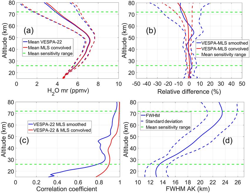
1104 G. Mevi et al.: VESPA-22
Trec (ν) Table 2. Mean values and SDs of Tsurf − Ttrop obtained from the
Thot (Vcold (ν) − V0 (ν)) − Tcold (Vhot (ν) − V0 (ν)) radiosoundings.
= , (12)
Vhot (ν) − Vcold (ν)
and Month Mean (Tsurf − Ttrop )
Vcold + nd (ν) − Vcold (ν) Jul 14.4 ± 2.8 K
Tnd (ν) = . (13) Nov 8.3 ± 3.6 K
α (ν)
Dec 9.4 ± 3.8 K
Thot and Tcold and Vhot and Vcold are the emission temper- Feb 9.4 ± 2.1 K
atures and the recorded count numbers of the two sources,
respectively. For the black body, the emission temperature is
assumed to be equal to its physical temperature. four periods, as described in Table 2. Ttrop is the average tem-
The noise diode produces a signal that is measured to be perature obtained from radiosonde data by weighting the tro-
quite stable in frequency. In fact, single-channel Tnd values pospheric temperature vertical profile with the water vapor
are always within 1.5 % of the spectral mean of the diode concentration profile. Using Eq. (15), it is possible to ex-
temperature brightness T nd . The spectra originated from plicitly give the relation between the opacity and the mean
black-body measurements (especially those from the CV-3 brightness temperature of the received signal:
immersed in LN2 ) can be affected by standing waves and in !
order to avoid to transfer them in the calibrated sky spec- T0 − Ttrop
tral measurements, Tnd is averaged over the central 11 000 µ (θi ) τ = ln . (17)
T (θi ) − Ttrop
channels of the FFTS, as suggested by Gomez et al. (2012).
Therefore, it can be written A linear regression of the opacities ln
T0 −Ttrop
ob-
T (θi )−Ttrop
X Vcold + nd (νi ) − Vcold (νi ) served at θi and the air mass factors µ (θi ) allows us to re-
T nd = (Thot − Tcold ) , (14)
i
Vhot (νi ) − Vcold (νi ) trieve the opacity at the zenith, τ (Nedoluha et al., 1995).
Substituting for T (θi ) using Eq. (8) and approximating all
where Vcold + nd (νi ) is the value of channel i with the noise the spectral quantities with their mean values (indicated by
diode turned on, while Vcold (νi ) is the value of the same a bar) over the central 11 000 channels, Eq. (17) can be writ-
channel with the noise diode turned off. ten as
3.4 Tipping curve procedure T0 − Ttrop
µ (θi ) τ = ln , (18)
V (θi )−V 0
In this section, the tipping curve calibration technique em- α − T rec − Ttrop
ployed to calibrate the noise diodes using the sky signal is
described. The tipping curve procedure is performed twice where it appears that the mean values T rec and α are needed
every hour as it is also used to measure the atmospheric opac- to perform the calculation.
ity needed in Eq. (9). During a tipping curve, VESPA-22 col- The emission from two calibration sources at different
lects the radiation coming from different elevation angles, temperatures is used to calculate α and T rec according to
approximately every 5◦ from 35 to 60◦ above the horizon. Eqs. (11) and (12). However, since the sky emission tem-
sky
The measured spectra are averaged using the 11 000 central perature Tcold is not known, an iterative procedure is used
channels of the spectrometer. Radiation from the stratosphere sky
to obtain both τ and Tcold . An initial opacity value, τ0 , is
contributes less than 1 % and can be neglected, so the signal sky
adopted as a first guess to obtain Tcold,0 using Eq. (21) with
intensity can be described by means of the following equa-
sky
tion: θ = 60◦ . Tcold,0 is then used to obtain α0 and Trec0 by means
of Eqs. (11) and (12); µ (θi ) τ is calculated for different ele-
T (θi ) ∼
= T0 e−µ(θi )τ + Ttrop 1 − e−µ(θi )τ . (15) vation angles using Eq. (18), and ultimately a linear fit allows
us to calculate a new estimate for τ , τ1 . The iterative proce-
The atmospheric temperature Ttrop can be estimated from the dure goes on until the intercept value is minimized. Figure 3
surface temperature Tsurf : shows the results of a tipping curve measurement carried out
Ttrop = Tsurf − d, (16) on 10 December 2016.
sky
The value of Tcold measured with this procedure is used in
where the value of d can be affected by seasonal variations. Eqs. (11) and (13) to estimate T nd . In order to avoid the use
In order to characterize this parameter several radiosound- of data acquired during inhomogeneous sky conditions, all
ings were launched during July, November, and Decem- measurements producing linear fits (see Fig. 3a) with a root
ber 2016 and February 2017. The value of the parameter d as mean square larger than 0.4 are discarded. Figure 4 shows
a function of time is obtained from a linear interpolation be- the time series of both noise diodes’ mean emission temper-
tween the mean values of Tsurf − Ttrop measured during these atures (blue and cyan) and their ratio (green dots and right
Atmos. Meas. Tech., 11, 1099–1117, 2018 www.atmos-meas-tech.net/11/1099/2018/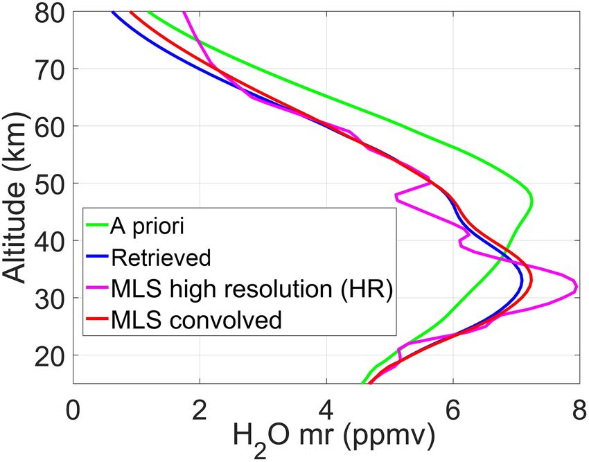
G. Mevi et al.: VESPA-22                                                                                                                          1105


                                       T0 −Ttrop
Figure 3. (a) The values of ln                           (indicated with τsig on the y axis of panel a) as function of the air mass factor µ (θi ) (blue
                                     T (θi )−Ttrop
points) measured during a tipping curve on 10 December 2016, and the fit result (green line). (b) The residuals (measurements minus fit) as
a function of the elevation angle.

Figure 4. Time series of the noise diodes mean emission temperature calculated by means of the tipping curve procedure (blue and cyan
solid circles) compared with values obtained by means of LN2 calibrations (orange and red stars). The green dots and the right y axis display
the ratio of the emissions from two noise diodes.

y axis) from July 2016 to July 2017. The noise diode in blue                       uncertainty on such a ratio is 0.05 (3.4 %), there appears to
is the one used as calibration diode. In the same plot, T nd val-                  be no drift in the time frame discussed in this work.
ues obtained using a LN2 cooled CV-3 as the cold load are
also depicted (orange and red stars). The mean relative dif-
ference between T nd values calculated with LN2 and with                           4   Retrieval process
tipping curves carried out immediately before or after LN2
calibrations is (0.4 ± 0.4) and (0.2 ± 0.3) % for the calibra-                     VESPA-22 water vapor vertical profiles are obtained us-
tion and the backup diodes, respectively. The ratio between                        ing the optimal estimation theory (Rodger, 2000). In what
the two noise diodes can provide insights into potential drifts                    follows the retrieved water vapor profile is indicated as x,
of one diode with respect to the other. Since the estimated                        whereas x a indicates the a priori profile and e
                                                                                                                                  x the real water
                                                                                   vapor atmospheric profile. The quantities y and y a represent

www.atmos-meas-tech.net/11/1099/2018/                                                                  Atmos. Meas. Tech., 11, 1099–1117, 2018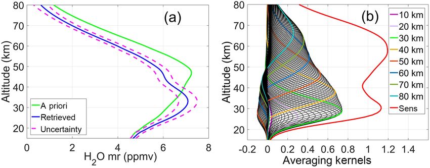
1106                                                                                                    G. Mevi et al.: VESPA-22

                                                                     For a 24 h integration time the Se diagonal values range from
                                                                     3×10⁻⁴ K2 (maximum value during summer) to 8×10⁻⁶ K2
                                                                     (minimum value obtained during winter).
                                                                        A second-order polynomial (light blue curve in Fig. 7a)
                                                                     is also added to the retrieval in order to take into account
                                                                     the spectral emission from the upper troposphere and lower
                                                                     stratosphere, as well as a potential contribution to the base-
                                                                     line from the delrin sheet. The polynomial is calculated in-
                                                                     dependently for each retrieved profile. The addition of this
                                                                     extra degree of freedom to the retrieval process reduces the
                                                                     altitude interval in which VESPA-22 retrievals can be consid-
                                                                     ered reliable, raising the lower limit of the sensitivity range
Figure 5. The value of σi used to compute the a priori covariance    (see definition below and Fig. 8b) by approximately 6 km al-
matrix as a function of altitude (Eq. 20).                           titude. The use of a second-order term also introduces an ad-
                                                                     ditional source of uncertainty into the retrieved mixing ratio
                                                                     profile. Such a contribution is taken into account in the error
the measured and a priori spectra, respectively. The matrix K        analysis discussed in Sect. 4.3 (see Fig. 11).
is the weighting functions matrix, whereas Se and Sa are the            An important quantity used to characterize the retrieval
covariance matrices associated to the spectral measurements          quality is the averaging kernels matrix A (Rodgers, 2000).
and the a priori vertical profile, respectively. The profile x       The rows of A are called averaging kernels (AKs) and can
can be used to calculate the synthetic spectrum y fit accord-        be used to characterize the sensitivity of the water vapor re-
ing to                                                               trieval at a given altitude to variations in the water vapor con-
y fit = y a + K (x − x a ) .                                 (19)    centration profile at all altitudes (Rodger, 2000). If the AKs
                                                                     are well-peaked functions, centered at their nominal altitude,
The altitude grid used for VESPA-22 retrievals starts from           a perturbation in the atmospheric water vapor concentration
10 km and goes up to 110 km altitude, at steps of 1 km. This         at a specific altitude is transferred by the algorithm to the
range is much larger than the sensitivity interval of the in-        correct altitude layer of the retrieved profile. Furthermore,
strument, which is in fact limited by the Doppler broadening         the area enclosed under each AK is an indication of the to-
at high altitudes and by the FFTS bandwidth and the tropo-           tal sensitivity of the retrieved value at that altitude to atmo-
spheric influence on the lower stratosphere at low altitudes.        spheric variations in water vapor concentration. A sensitivity
Only the central 400 MHz of the measured spectrum are used           value close to 1 at a certain altitude indicates that the major
in the retrieval. The Sa matrix is computed according to             contribution to the retrieved value at that altitude comes from
                                                                     the spectral measurements rather than from the a priori wa-
                   |
                  − zi −zj   |
Sa,ij = σi σj e       h          ,                           (20)    ter vapor profile. Following what was indicated by Tschanz
                                                                     et al. (2013), VESPA-22 retrievals are also considered valid
where σi is the root mean square of the variance of the a            for scientific use in the altitude range where the sensitivity
priori profile (expressed in volume mixing ratio, or vmr; see        is above 0.8. The AKs’ FWHM can be used as a rough es-
Fig. 5) at the altitude zi , while h is a correlation altitude set   timate of the local vertical resolution of the obtained water
to be 5 km. Values of σi were empirically chosen in order            vapor mixing ratio vertical profile.
to optimize the characteristics of the retrieval (i.e., maximize
sensitivity range and vertical resolution without introducing        4.1   Forward model and a priori profiles
unphysical oscillations in the retrieved vertical profile).
   In the inversion process for VESPA-22 spectra, Se is a di-        Figure 6 displays the a priori profiles used by the VESPA-
agonal matrix with its diagonal elements all equal and calcu-        22 retrieval algorithm during 10 out of the 12 months of the
lated using a two-step process. A first retrieval of the origi-      year and based on local climatology (3 years’ worth of data
nal, not smoothed (see Sect. 3.2), spectral measurement av-          of Aura/MLS v4.2). These profiles are identical below 48 km
eraged over 24 h is performed using a fixed value (1 × 10⁻⁵ )        and diverge above, due to the large difference in polar re-
for the Se diagonal elements and the obtained profile, x0 ,          gions between summer and winter water vapor mesospheric
is used to calculate a synthetic spectrum y 0,fit by means           profiles. The summer a priori (red line) is used during the
of Eq. (19). In order to consider the spectral measurement           period from 1 June to 15 September, while the winter a pri-
noise in the retrieval process, a second and final inversion         ori (blue line) is used during the period from 16 October to
is then performed, this time with the Se diagonal elements           30 April. During the month of May and from 16 September
                                 2
set to the y unsmoothed − y 0,fit mean value and the spectrum        to 15 October, there are transition periods in which a linear
smoothed as indicated in Sect. 3.2. Note that also in this sec-      daily interpolation from one a priori to the other was used for
ond inversion the diagonal elements of Se are held constant.         continuity.

Atmos. Meas. Tech., 11, 1099–1117, 2018                                                www.atmos-meas-tech.net/11/1099/2018/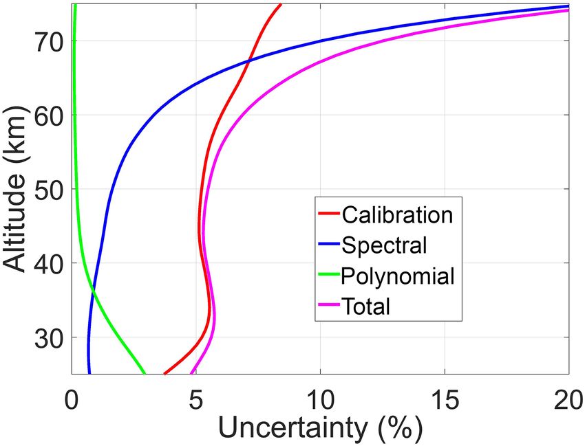
G. Mevi et al.: VESPA-22                                                                                                             1107

Table 3. Spectroscopic parameters (“reference” model) used for VESPA-22 retrievals. Indicated parameters, from left to right, are emission
line frequency, intensity, lower state energy, pressure broadening coefficient, pressure broadening temperature dependence, self-broadening
coefficient, and self-broadening temperature dependence. The line intensity is given for a reference temperature of 296 K.

                    ν0                       S                   E                γair       nair     γself      nself
                    (GHz)                 (m2 Hz)                (J)           (Hz Pa−1 )           (Hz Pa−1 )
                    22.235043990      5.3648 × 10⁻¹⁹       8.869693 × 10⁻²¹      28 110      0.69    134 928       1
                    22.235077056      4.5703 × 10⁻¹⁹       8.869693 × 10⁻²¹      28 110      0.69    134 928       1
                    22.235120358      3.9740 × 10⁻¹⁹       8.869693 × 10⁻²¹      28 110      0.69    134 928       1

                                                                        diosoundings launched from the Eureka station, PWVEu is
                                                                        the associated water vapor column content, and PWVHatpro is
                                                                        the column content measured by the HATPRO located at the
                                                                        THAAO. Data from Eureka were chosen (instead of those
                                                                        from Alert, Canada, for example) because they show the
                                                                        closest resemblance to the tropospheric profiles measured at
                                                                        Thule by local radiosoundings, when the latter are available.
                                                                        In order to avoid discontinuities in x ARTS , values at altitudes
                                                                        between 9 and 12 km are obtained with a linear interpolation
                                                                        between x ARTS (9 km) and x ARTS (12 km).
                                                                            The pressure and temperature profiles needed to run the
                                                                        forward calculation are built merging NASA Goddard Space
Figure 6. The a priori profiles employed by VESPA-22 for the            Flight Center (GSFC), Aura/MLS and climatological tem-
October–April period (indicated as winter a priori, blue line) and      perature and pressure profiles. The NASA GSFC profiles ob-
for the June–August period (indicated as summer a priori, red line)     tained through the Goddard Automailer Service (Lait et al.,
obtained from climatology.                                              2005) are used to build the tropospheric meteorological
                                                                        state, from the ground up to 9 km of altitude. Between 10
                                                                        and 87 km altitude, the MLS temperature and pressure pro-
   The matrix K and the y a spectrum are calculated using
                                                                        files collected during VESPA-22 observations, in a radius of
the radiative transfer simulation software ARTS (Eriksson
                                                                        300 km from the observation point of VESPA-22, are aver-
et al., 2011), adopting a Voigt–Kuntz lineshape and the line
                                                                        aged together to produce a single set of daily meteorological
intensity provided by the JPL 2012 catalogue (Pickett et al.,
                                                                        vertical profiles. The VESPA-22 observation point coordi-
1998, and https://spec.jpl.nasa.gov/). Following the work of
                                                                        nates are chosen to be 74.8◦ N and 73.5◦ W, and represent an
Seele (1999) and Tschanz et al. (2013), the line described
                                                                        estimate of the geographical coordinates of the air mass that
by the JPL 2012 catalogue is divided into three emission
                                                                        is observed by VESPA-22 (which points southwest, at about
lines indicating the hyperfine splitting of the 22.235 GHz wa-
                                                                        220◦ ) at 60 km altitude when the instrument aims at an ele-
ter vapor line. The employed pressure broadening and self-
                                                                        vation of 15◦ above the horizon. Daily temperature and pres-
broadening parameters are those reported by Liebe (1989).
                                                                        sure profiles from 97 to 110 km of altitude are obtained by
Table 3 summarizes the spectroscopic parameters used for
                                                                        daily smoothing zonal monthly averages from the COSPAR
the analysis of VESPA-22 spectral measurements which, in
                                                                        International Reference Atmosphere (Fleming et al., 1990).
what follows, are indicated as the “reference” model.
                                                                            The absence of vertical discontinuities in the temperature
   The profile x ARTS is the profile used in the forward model
                                                                        and pressure daily profiles is assured by a smoothing process
calculations to compute the a priori spectrum and the weight-
                                                                        performed at the altitudes where the three different datasets
ing functions. x ARTS matches the a priori profile from 12 km
                                                                        (GSFC, MLS, and COSPAR) are stitched together, between
of altitude upward and, below 9 km, it is consistent with the
                                                                        9 and 12 km and between 87 and 97 km.
measurements of precipitable water vapor (PWV) collected
                                                                            The software ARTS is employed to simulate the emission
by the HATPRO radiometer (Rose and Czekala, 2009; Pace
                                                                        from the zenith, e y r , and from an angle close to the horizon,
et al., 2015) installed at the THAAO. This lower part of
                                                                        y s . The emission e
                                                                                           y r is then rescaled using Eq. (22), therefore
x ARTS is calculated according to
                                                                        simulating the effect of the delrin compensating sheet:
                                        PWVHatpro
                                                                               y r + Td 1 − e−τd ,

x ARTS (from the ground to 9 km) =                x Eu ,       (21)     yr = e                                                       (22)
                                         PWVEu
                                                                        whereas the mean difference y s − y r is
where x Eu is a water vapor mixing ratio profile obtained by
                                                                                         µe
                                                                                          τ       τ −τd
                                                                                     µe−e     − e−e

daily smoothing monthly averages calculated from the ra-                ys − yr = ya e                  .                             (23)

www.atmos-meas-tech.net/11/1099/2018/                                                       Atmos. Meas. Tech., 11, 1099–1117, 2018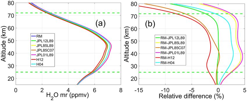
1108                                                                                                      G. Mevi et al.: VESPA-22

The opacity τd used in Eq. (22) is the opacity of the com-            Table 4. Uncertainties on the various parameters used in the cali-
pensating sheet; the temperature Td is the temperature of the         bration process. When the uncertainty is a function of altitude the
sheet, measured by a sensor installed next to it; and the signal      minimum and maximum values of the uncertainty are reported.
beam observing angle, e  θ , is chosen in order to minimize the
mean difference y s −y r , as it is in fact attained by VESPA-22       Parameter                                             Uncertainty
in its data-taking process. The a priori spectrum is calculated                                                    (relative or absolute)
according to the same equation used for the measured signal            Signal angle, θ                                          ±0.1◦
(Eqs. 5 and 6),                                                        Noise diode brightness temperature, Tnd                 ±1.7 %
                                                                       Atmospheric opacity at the zenith, τ                     ±5 %
          ys − yr                                                      Air temperature profile                          [±2.1 ± 5.0] K
ya =      µ
         −eτ − e−eτ −τd
                        ,                                     (24)
       µe e
       e                                                               Geopotential height                              [±30 ± 110] m
                                                                       Delrin opacity, τd                                      ±10 %
where e µ and e  τ are the air mass factor associated to the simu-
                                                                       Spectroscopic parameters                         [±1 % ± 10 %]
lated signal beam and the zenith opacity calculated from the
x ARTS profile.
   Deriving Eqs. (24) and (22), and using the K matrix defini-
tion (Rodgers, 2000), the retrieval weighting function matrix         the real atmospheric concentration profiles. In discussing the
can be written as                                                     optimal estimation method, Rodgers (2000) suggests that this
                                                                    error, called “smoothing error”, should be estimated only if
       ∂           ys − yr                                            accurate knowledge of the variability of the atmospheric fine
K=                 µe
                    τ − e−e  τ −τd
      ∂x e   µe−e                   xa                                structure is available. This approach is used here and the
      h i
        ∂y s
                    h i
                      ∂y r                                            smoothing error is not included in the error estimate.
        ∂x x − ∂x x                  Ks − Kr e−τd                        The first contribution can be evaluated observing the dif-
   ∼
   =           a             a
                                = −e                 ,         (25)
       µe
       e   −eµτ
              e  −e  −eτ −τd       µe µe
                                   e    τ − e−eτ −τd                  ference 1ylin between the fit spectrum without the addition
                                                                      of the second-order polynomial, y ∗fit , and the spectrum ob-
where Ks and Kr are the weighting function matrices that              tained using ARTS to calculate the emission expected from
ARTS calculates for the simulated signal and reference                the retrieved profile x (in the calculation, ARTS does not per-
beams. As a first approximation, the dependence of e  τ on the        form any linear approximation):
stratospheric water vapor profile in Eq. (25) is neglected.
                                                                      1ylin = y ∗fit − f (x).                                        (26)
4.2    Retrieval example
                                                                      The uncertainty 1xlin that 1ylin causes on the retrieved pro-
Figure 7a shows a VESPA-22 spectrum integrated for 24 h               file can be calculated with
(blue line) on 23 December 2016, its corresponding synthetic
spectrum y fit (red line) and the a priori spectrum (green line),     1xlin = G1ylin ,                                               (27)
while the residual (defined as the difference between fit and
measured spectrum, y fit − y) is plotted in Fig. 7b. The cyan         where G is the gain matrix (Rodgers, 2000). The uncertainty
line is the second-degree polynomial retrieved by the inver-          1xlin has a negligible contribution to the total uncertainty
sion algorithm. Figure 8a shows the result of the inversion           (with a maximum of 0.1 % at 70 km altitude).
of the measured spectrum depicted in Fig. 7 with the a priori            Figure 8b shows the corresponding averaging kernels
profile and retrieval 1σ uncertainty. The details on the uncer-       (AKs, black and colored solid lines). AKs are multiplied by
tainty calculation are discussed in Sect. 4.3.                        a factor of 10 and the sensitivity in indicated with a red solid
                                                                      line.
4.3    Retrieval uncertainty                                             In order to evaluate the second contribution listed above,
                                                                      the effects on the retrieved profile due to the variation of each
The uncertainty characterizing VESPA-22 retrieved profiles            single parameter used in the measurements calibration and
can be divided into four major contributions: (1) the un-             pre-processing was investigated. The difference between the
certainty due to the linear approximation used in the opti-           profile retrieved using the “correct” value of a specific pa-
mal estimation, (2) the uncertainty due to the various pa-            rameter and the retrieval obtained by changing such a value
rameters used in the spectra calibration and pre-processing,          by the estimated relative uncertainty of the parameter is con-
(3) the uncertainty due to spectral noise and potential arti-         sidered to be the contribution σi of this parameter to the to-
facts, and (4) the uncertainty introduced by the use of the           tal calibration and pre-processing uncertainty. The total un-
second-order polynomial in the retrieval process. One addi-           certainty from these sources is defined as calibration uncer-
tional error source is the limited vertical resolution inher-         tainty. Table 4 summarizes the uncertainties on the various
ent to concentration vertical profiles obtained by means of           parameters involved in the calibration and pre-processing of
this ground-based observing technique. This leads to solu-            VESPA-22 spectra. When the uncertainty is a function of al-
tion profiles that can be considered a smoothed version of            titude the minimum and maximum values of the uncertainty

Atmos. Meas. Tech., 11, 1099–1117, 2018                                                  www.atmos-meas-tech.net/11/1099/2018/
G. Mevi et al.: VESPA-22 1109
Figure 7. (a) An example of VESPA-22 measured spectrum (blue) collected on 23 December 2016, with the a priori spectrum in green and
the fit spectrum in red. The second-order polynomial is indicated with a cyan solid line. (b) The residual y fit − y. The central part of the
spectrum is unsmoothed in order to maintain the maximum spectral resolution near the peak and its residual is larger.
Figure 8. (a) The retrieved VESPA-22 profile (blue solid line) correspondent to the spectrum showed in Fig. 7. The a priori profile is indicated
with a green solid line. The two red dashed lines describe the uncertainty of this VESPA-22 retrieval (for details on the estimated uncertainty
of VESPA-22 mixing ratio vertical profiles see Sect. 4.3). (b) Rows of the A matrix multiplied by a factor of 10 as a function of altitude
(some A functions are highlighted in colors). The vertical profile of the sensitivity is shown in red.
are reported. The total calibration uncertainty σcal is given by water vapor mixing ratio vertical profile due to the uncer-
sX tainty on the estimated noise diode temperature T nd . In order
σcal = σi2 . (28) to evaluate the uncertainty on T nd , the 0.4 % difference be-
i tween the values obtained by means of the LN2 calibrations
and by means of the skydips immediately following or pre-
ceding the LN2 calibrations (see Sect. 3.4 and Fig. 4) is con-
In Fig. 9, the relative contributions of the various parame-
sidered. On top of this, the fluctuations of the signal produced
ters needed in the calibration and pre-processing procedures
by the calibration diodes must also be taken into account.
are shown. The yellow line shows the σi contribution due to
These can be evaluated by using the standard deviation (SD)
the uncertainty on the signal beam angle. In order to mini-
of the difference over time between the T nd values of the
mize this contribution, the choked antenna and the parabolic
two noise diodes, measured to be 1.1 %. The tipping curve
mirror are aligned using a He-Ne laser. During the period
procedure allows for calculation of the noise diodes bright-
from April to October, the VESPA-22 pointing offset can be
ness temperature averaged over the 11 000 central channels
verified by scanning rapidly at around the sun elevation an-
of the spectrometer. Since the noise diodes brightness tem-
gle and comparing the measured position of the center of the
peratures do have a small frequency dependence, using their
sun against the known ephemerides. For the measurements
mean values introduces a source of uncertainty which is es-
discussed here an offset of 1θ = 0.2◦ ± 0.1◦ was estimated.
timated to be 0.9 %. An additional source of uncertainty is
The green solid line shows the potential relative error on the
www.atmos-meas-tech.net/11/1099/2018/ Atmos. Meas. Tech., 11, 1099–1117, 20181110 G. Mevi et al.: VESPA-22
May 2017 using different sets of values for the spectro-
scopic parameters (see also Haefele et al., 2009). In the fig-
ure, the mean profiles retrieved using the different models
listed in the legend are depicted. Such models include values
taken from HITRAN (Rothman et al., 2013) and JPL cat-
alogues (Pickett et al., 1998), for different years, and from
Liebe (1989) and Cazzoli et al. (2007). The blue line repre-
sents the mean profile obtained using VESPA-22 reference
model (RM). In Fig. 10b, the mean relative difference pro-
files between retrievals obtained using the reference model
and the other spectroscopic models are drawn (see legend).
The water vapor mixing ratio retrieved profiles show a strong
dependence on the spectroscopic model of choice, with a rel-
Figure 9. Relative contributions to the calibration uncertainty de- ative difference between profiles obtained using different
fined by Eq. (28) and indicated with a red solid curve. The contri- models reaching a maximum of 8 % at the top of the sen-
butions are the signal beam angle (yellow), the noise diode tempera- sitivity range.
ture (green), the sky opacity (blue), the MLS meteorological profiles
Figure 11 shows the uncertainty calculated for the retrieval
(orange and brown), the compensating sheet opacity (magenta), and
of 23 December 2016, shown in Fig. 8. The overall calibra-
the spectroscopic parameters (cyan).
tion uncertainty is shown with a red curve. The uncertainty
due to spectral noise and artifacts can be evaluated using the
S uncertainty matrix (Rodger, 2000) obtained as
due to sky inhomogeneities, and amounts approximately to −1
1 %. All these sources of uncertainty for T nd are added in S = KT S−1 e K + Sa
−1
. (29)
quadrature to obtain a total uncertainty of 1.8 %. The blue
line shows the contribution due to the uncertainty 1τ on the
sky zenith opacity τ . In order to estimate this uncertainty, The square root of the diagonal elements of S represents
the uncertainties introduced by sky inhomogeneity and by the spectral uncertainty of the retrieved profile at different
the estimation of the effective tropospheric temperature Ttrop altitudes and is indicated in Fig. 11 with a blue line. This
are considered. The first contributes to about 2 % and is es- term depends on the Se value of the retrieval and its value
timated using the uncertainty on the slope of the linear fit of increases during summer and with poor weather conditions.
the tipping curve (see Sect. 3.4 and Fig. 3). The second con- As mentioned in Sect. 4, the diagonal values of the Se ma-
tribution can be evaluated observing the daily fluctuations of trix are held constant and do not take into account the spec-
Ttrop measured at Eureka (Canada), Aasiaat (southern Green- tral noise reduction obtained with the 50-channel smoothing
land), and Alert (Canada). The natural day-to-day tempera- process which is applied to most of the spectrum (Sect. 3.2).
ture fluctuations and the lack of tropospheric meteorological This may lead to a small overestimation of the spectral un-
data at Thule during long intervals of time led us to estimate certainty depicted in Fig. 11 in the altitude range 20–50 km
an uncertainty on Ttrop of about 6 K, which then makes the (with a maximum potential overestimation of 0.3 % at 25 km
total uncertainty 1τ ∼5 %. altitude). The green curve displays the estimated uncertainty
The brown and orange lines show the σi ’s due to temper- due to the use of the second-order polynomial in the retrieval
ature and geopotential height profiles used in the forward process. The total uncertainty is calculated as
calculation. The uncertainties on these parameters are ob- q
2 +σ2 +σ2
σtot = σcal spec poly (30)
tained from the MLS data quality and description document
(Livesey et al., 2015). In Fig. 9, the magenta line shows the and is represented with a purple line in Fig. 11.
contribution of the uncertainty on the compensating sheet
opacity, 1τd . Although the uncertainty on the measurements
of τd is about 2 % (see Table 1), the use of a linear interpola- 5 VESPA-22 and Aura/MLS water vapor profile
tion suggests the use of a more conservative estimate, eventu- intercomparison
ally set at 10 %. The cyan line shows the contribution due to
uncertainties in the employed spectroscopic parameters, and VESPA-22 water vapor vertical retrievals obtained from 24 h
it has the largest impact on the calibration uncertainty. Fol- integration spectra (from 00:00 to 23:59 UT) have been com-
lowing Straub et al. (2010), the emission line intensity and pared with version 4.2 of Aura/MLS water vapor vertical
the pressure broadening coefficient were assigned an uncer- profiles. The MLS profiles used for this intercomparison are
tainty of 8.7 × 10⁻²² m2 Hz and 1014 Hz Pa−1 , respectively. daily mean profiles obtained averaging all MLS profiles col-
In addition to these uncertainties, Fig. 10 shows the re- lected within a radius of 300 km centered around VESPA-22
sults of retrieving VESPA-22 data from October 2016 to observation point (74.8◦ N, 73.5◦ W; see Sect. 4.1).
Atmos. Meas. Tech., 11, 1099–1117, 2018 www.atmos-meas-tech.net/11/1099/2018/G. Mevi et al.: VESPA-22 1111
Figure 10. (a) Mean retrieved water vapor profiles obtained using different spectroscopic models (the blue line is the model eventually
adopted for the analysis of VESPA-22 spectra, called reference model, or RM). The spectroscopic parameters for the additional models
tested are obtained from different versions of the JPL catalogue (years 1985, 2001 and 2012; Pickett et al., 1998) with the pressure broadening
parameters taken from Liebe (1989) and Cazzoli et al. (2007). Two models include values from HITRAN 2004 and 2012 (Rothman et al.,
2013). Models are indicated in the legend with their abbreviations: JPL2012Liebe1989 (JPL12L89), JPL1985Liebe, 1989 (JPL85L89),
JPL1985Cazzoli, 2007 (JPL85C07), JPL2001Liebe, 1989 (JPL01L89), HITRAN2012 (H12), and HITRAN2004 (H04). (b) Vertical profiles
of mean relative differences between VESPA-22 profiles obtained using the reference model and the different spectroscopic models. Data
represented here range from 4 October 2016 to 22 May 2017. The average retrieval sensitivity range is marked by dashed horizontal green
lines.
erence beam window. A few isolated days in which large sky
inhomogeneities do not allow the correct balance of signal
and reference beams have also been removed from the in-
tercomparison. It is worth recalling that the signal-to-noise
ratio of VESPA-22 spectra, and therefore the quality of the
retrievals, depends on the sky opacity and, consequently, on
the season, being noticeably better during winter and poorer
in summer. This is particularly true for microwave spectrom-
eters operating in polar regions, where seasonal fluctuations
of the tropospheric water vapor column content are signifi-
cant.
Table 5 summarizes the characteristics of the Aura/MLS
water vapor version 4.2 retrievals (Livesey et al., 2015). In
Figure 11. Vertical profiles of the calibration uncertainty (red), the order to compare the two datasets, MLS vertical profiles
retrieval uncertainty (blue), and the total uncertainty (magenta) of are convolved with VESPA-22 averaging kernels in order
VESPA-22 water vapor mixing ratio vertical profiles obtained in-
to match the resolution of VESPA-22 profiles according to
verting a spectrum collected on 23 December 2016 and integrated
for 24 h.
Rodgers (2000):
x MLS = x a + A e
x MLS − x a , (31)
The intercomparison is carried out using data from
15 July 2016 to 2 July 2017. In general, spectra collected where ex MLS is the raw (high resolution or HR) MLS water
during July, August, and September are less continuous and vapor vertical profile, x a is the a priori profile, A is the aver-
noisier than spectra observed during the rest of the selected aging kernel matrix, and x MLS is the convolved MLS profile.
period. This is due to extensive testing of the equipment, poor Additionally, VESPA-22 profiles were also compared with
weather conditions, and snow covering the zenith observing MLS profiles smoothed in the vertical by using a 10 km mov-
window (in November 2016 a second powerful fan was in- ing average. This second set of degraded MLS profiles was
stalled outside the roof window in order to reduce snow de- generated in order to study the correlation between VESPA-
position). Furthermore, there are no stratospheric measure- 22 and MLS datasets without introducing the dependency
ments carried out by VESPA-22 between 4 and 22 Novem- from one another brought by the convolution process (affect-
ber 2016, due to snow covering the lower portion of the ref- ing MLS convolved profiles).
www.atmos-meas-tech.net/11/1099/2018/ Atmos. Meas. Tech., 11, 1099–1117, 2018You can also read