Reanalysis of the PacIOOS Hawaiian Island Ocean Forecast System, an implementation of the Regional Ocean Modeling System v3.6
←
→
Page content transcription
If your browser does not render page correctly, please read the page content below
Geosci. Model Dev., 12, 195–213, 2019
https://doi.org/10.5194/gmd-12-195-2019
© Author(s) 2019. This work is distributed under
the Creative Commons Attribution 4.0 License.
Reanalysis of the PacIOOS Hawaiian Island Ocean Forecast System,
an implementation of the Regional Ocean Modeling System v3.6
Dale Partridge, Tobias Friedrich, and Brian S. Powell
University of Hawai‘i at Mānoa, Department of Oceanography, Marine Sciences Building,
1000 Pope Road, Honolulu, Hawai‘i 96822, USA
Correspondence: Brian S. Powell (powellb@hawaii.edu)
Received: 7 April 2018 – Discussion started: 4 July 2018
Revised: 1 November 2018 – Accepted: 8 November 2018 – Published: 9 January 2019
Abstract. A 10-year reanalysis of the PacIOOS Hawaiian get (Souza et al., 2015). In this work, we perform an extended
Island Ocean Forecast System was produced using an in- reanalysis from 2007 to 2017 in order to produce a consistent
cremental strong-constraint 4-D variational data assimilation dataset for further studies of the dynamics around Hawai‘i.
with the Regional Ocean Modeling System (ROMS v3.6). The PacIOOS forecast system uses the time-dependent
Observations were assimilated from a range of sources: incremental strong-constraint four-dimensional variational
satellite-derived sea surface temperature (SST), salinity data assimilation (I4D-Var) scheme (Courtier et al., 1994;
(SSS), and height anomalies (SSHAs); depth profiles of tem- Moore et al., 2004) within the Regional Ocean Modeling
perature and salinity from Argo floats, autonomous Seaglid- System (ROMS) (Moore et al., 2011c; Powell et al., 2008;
ers, and shipboard conductivity–temperature–depth (CTD); Matthews et al., 2012) to best reduce the residuals between
and surface velocity measurements from high-frequency the model and observations, while maintaining a physically
radar (HFR). The performance of the state estimate is exam- consistent solution. The class of methods known as 4D-Var
ined against a forecast showing an improved representation are state-estimation techniques that create a quadratic cost
of the observations, especially the realization of HFR surface function to be minimized over a defined time window utiliz-
currents. EOFs of the increments made during the assimila- ing observations at the time they occur in a physically con-
tion to the initial conditions and atmospheric forcing com- sistent manner to adjust the initial state, boundary conditions,
ponents are computed, revealing the variables that are influ- and atmospheric forcing to represent the measurements. The
ential in producing the state-estimate solution and the spatial I4D-Var scheme is used in operational centers around the
structure the increments form. world and solves for increments to the model state, boundary
conditions, and atmospheric forcing using the model physics
as a constraint. The combination of I4D-Var within ROMS
has been used in previous studies of various regions (Pow-
1 Introduction ell et al., 2008; Broquet et al., 2009; Zhang et al., 2010;
Matthews et al., 2012; Souza et al., 2015). The details of the
The Pacific Integrated Ocean Observing System (PacIOOS, model and the observations used within this study are pro-
2018) has produced daily forecasts of the ocean state sur- vided in Sect. 2.
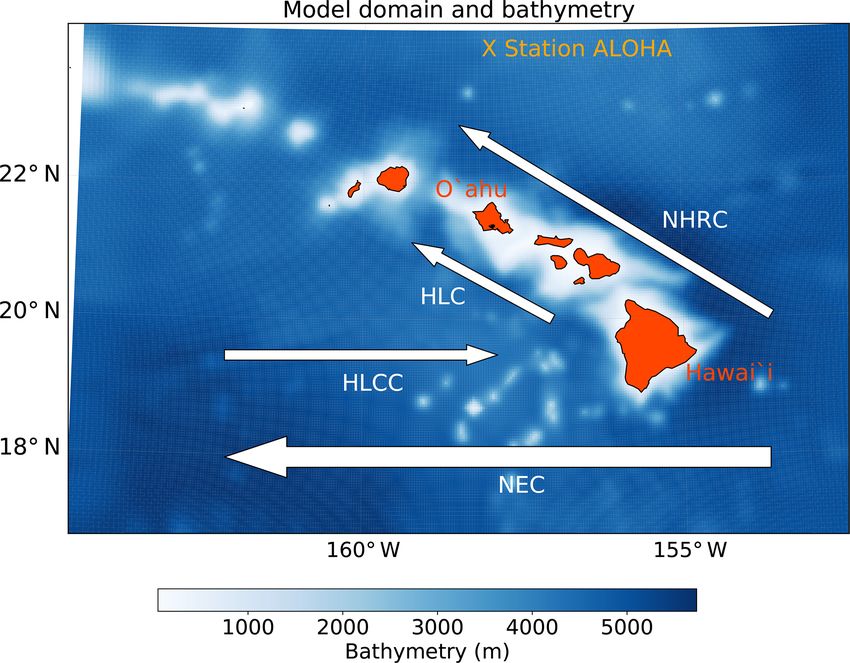
rounding the Hawaiian Islands since 2009. To facilitate the Our model domain covers the Hawaiian Island
forecasts a data assimilation procedure is used to incorporate Archipelago (Fig. 1), a dynamically active region for
recent observational data into the model to produce the opti- both the ocean and atmosphere. The North Equatorial Cur-
mal initial state from which to forecast. A number of model- rent (NEC), flowing from the east, splits upon encountering
ing studies have been performed with older versions of this the island of Hawai‘i, with the bulk transport traveling
model to examine various features of the modeling frame- around the south of the island and continuing west, while the
work, such as the state estimation (Matthews et al., 2012), North Hawaiian Ridge Current (NHRC) follows the ridge of
nested models (Janeković et al., 2013), and the vorticity bud-
Published by Copernicus Publications on behalf of the European Geosciences Union.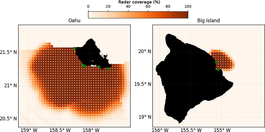
196                                                               D. Partridge et al.: Hawaiian Island Ocean Forecast System

                                                                    forcing to determine how the model is adjusted. By evalu-
                                                                    ating the empirical orthogonal functions (EOFs) of these in-
                                                                    crements we determine the spatial patterns in the variability.
                                                                    Since physical modes are not always independent (Simmons
                                                                    et al., 1983), the interpretation of EOF modes must be under-
                                                                    taken with some caution. As such the resulting modes will
                                                                    not necessarily represent a physical phenomenon, but will
                                                                    highlight the variable spatial patterns made over time by the
                                                                    I4D-Var algorithm.

                                                                    2     Numerical model and data assimilation system

                                                                    2.1    Model configuration

                                                                    The Regional Ocean Modeling System (ROMS) version 3.6
                                                                    is used to simulate the physical ocean around the Hawaiian
Figure 1. Model domain and bathymetry, with mean currents la-       Islands. ROMS is a free-surface, hydrostatic, primitive equa-
beled from Lumpkin and Flament (2013).                              tion model using a stretched coordinate system in the verti-
                                                                    cal to follow the underwater terrain. In order to allow vary-
                                                                    ing time steps for the barotropic and baroclinic components,
                                                                    ROMS utilizes a split-explicit time stepping scheme (for
the other islands in the chain to the north. In the atmosphere,     more details on ROMS, see Shchepetkin and McWilliams,
there are persistent trade winds from the northeast that,           1998, 2003, 2005).
combined with steep mountainous terrain on the islands,                The Hawaiian Island domain covers 164–153◦ W longi-
cause wind wakes in lee of the peaks, particularly on the           tude and 17–23◦ N latitude, with bathymetry provided by the
islands of Hawai‘i and Maui. This introduces strong tem-            Hawaiian Mapping Research Group (HMRG, 2017), shown
perature gradients, increases the seasonal variability (Sasaki      in Fig. 1. The grid has 4 km horizontal resolution with 32
and Klein, 2012), and drives currents such as the Hawaiian          vertical s levels configured to provide a higher resolution in
Lee Countercurrent (HLCC) (Smith and Grubišić, 1993; Xie           the more variable upper regions. The configuration model,
et al., 2001; Chavanne et al., 2002).                               including the method for assimilating surface HFRs and the
   There are two main objectives to this study: to assess the       associated vertical stretching scheme, is identical to the one
skill and performance of the state-estimation model and to          first presented in Souza et al. (2015).
analyze the increments made to the initial, boundary, and at-          Tidal forcing is produced using the OSU Tidal Prediction
mospheric forcing terms. For the first objective, we compare        Software (OTPS) (Egbert et al., 1994), which is based on the
the state-estimate solution with a free-running forecast over       Laplace tidal equations from the TOPEX/Poseidon Global
the decadal time period and examine how the performance             Inverse Solution (TPXO). Tidal constituents included in this
changes over time utilizing observations derived from satel-        simulation are the eight main harmonics, M2 , S2 , N2 , K2 ,
lites and it situ measurements. In addition, PacIOOS operates       K1 , O1 , P1 , and Q1 , as well as two long-period and one non-
seven high-frequency radar stations sites across the Hawai-         linear constituent: Mf , Mm , and M4 . To avoid any long-term
ian Islands. The first station was constructed in 2010, with        drifting of the tidal phases related to constituents we do not
the remaining six becoming operational over the period from         consider, the tidal harmonics are updated each year to define
2011 to 2015. These instruments produce high-resolution             the phases in terms of the start of that year.
(both spatially and temporally) surface current velocities in          Lateral boundary conditions are taken from the HYbrid
the vicinity of the islands of O‘ahu and Hawai‘i. The use of        Coordinate Ocean Model (HYCOM) (Chassignet et al.,
HFR observations within a state-estimation scheme has been          2007) and are applied daily. Within ROMs, we apply the
shown to produce a significantly improved representation of         boundary differently for each variable; Chapman (Chapman,
surface currents (Souza et al., 2015; Kerry et al., 2016). The      1985) conditions are applied to the free surface, Flather
impact of the radar stations will be a key focal point. The         (Flather, 1976) conditions for transferring momentum from
performance assessment is achieved through the statistics           2-D barotropic energy out of the domain, and 3-D momen-
produced by the state estimation in Sect. 3, followed by a          tum and tracer variables are clamped to match HYCOM. A
comparison with observations in Sect. 4. The forecast skill,        sponge layer of 12 grid cells (48 km) linearly relaxes the vis-
a measure of the accuracy for a forecast system, is computed        cosity by a factor of 4 and diffusivity by a factor of 2 close
with reference to a persistence assumption (Sect. 5).               to the boundary to account for imbalances between HYCOM
   Section 6 focuses on the second objective of the paper, to       and ROMS.
examine the increments to the initial state and atmospheric

Geosci. Model Dev., 12, 195–213, 2019                                                  www.geosci-model-dev.net/12/195/2019/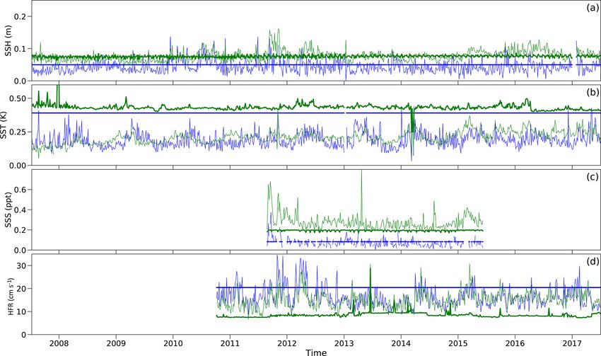
D. Partridge et al.: Hawaiian Island Ocean Forecast System                                                                     197

   From 2007 to 2009, atmospheric forcing fields (exclud-          tation of I4D-Var in ROMS is covered extensively in Moore
ing the wind) are provided by the National Center for Envi-        et al. (2011a, b, c).
ronmental Prediction (NCEP) reanalysis fields (Kistler et al.,
2001). For the wind forcing, a combination of two different        2.2     Experiment setup
forcings is utilized: (i) a 1/2◦ resolution CORA/NCEP wind
product (Milliff et al., 2004) that combines QuikScat mea-         The reanalysis covers a period of 10 years from July 2007 to
surements with NCEP wind fields and (ii) the CORA/NCEP             July 2017. The period of assimilation for the I4D-Var cycles
winds blended with the results from a 1/12◦ resolution             is 4 days, which corresponds to the limit of the linearity as-
PSU/NCAR mesoscale model (MM5; Yang et al., 2008a)                 sumption within the domain (Matthews et al., 2011). The at-
of the Hawaiian islands (Van Nguyen et al., 2010). The             mospheric forcing is adjusted every 6 h, while the boundaries
MM5 model was forced at its boundaries with the global             are every 12 h. An analysis of these adjustments is performed
NCEP fields; hence, it is a consistent dynamical downscal-         in Sect. 6.
ing of the global fields. The MM5 model domain is smaller             During each I4D-Var cycle, a minimization procedure is
than the ocean grid domain, extending only to 160.5◦ W in          applied. The nonlinear model is first integrated forward to
the lee. Therefore, for (ii), we must blend the modeled and        estimate the background state (the first outer loop). Then
CORA/NCEP winds to generate a consistent field for the en-         the tangent-linear and adjoint models are integrated in mul-
tire region with 1/12◦ winds where available and 1/2◦ winds        tiple inner loops to minimize the cost function (J ). After the
everywhere else.                                                   last inner loop the nonlinear model is updated (see Fig. 1
   To blend the two, we convert the MM5 winds to anoma-            of Moore et al., 2011c). Prior methodological experiments
lies by subtracting a 30-day mean centered about the record        yielded that for our setting a sufficient reduction in J (and
of interest. We compute the mean for the same period from          an acceptable computational cost) can be achieved using a
the CORA/NCEP winds. The difference between the two                single outer loop with 13 inner loops (Souza et al., 2015).
means provides a bias estimate. The bias is removed from              Several 4- and 8-day forecasts are performed from the end
the MM5 anomalies and the CORA/NCEP mean is added.                 of each cycle using the assimilated state as initial conditions,
Within a 1◦ box around the boundary of the MM5 data, we            and the short-range (1–4 days) and midrange (5–8 days) fore-
taper the anomalies to zero with a cosine filter to avoid abrupt   casts are evaluated for skill.
changes to the field. This step ensures that the mean of the
                                                                   2.3     Observations
CORA/NCEP field is preserved, while its structure and vari-
ability is greatly enhanced by the MM5.                            Observational data used within this study include satellite
   From July 2009, atmospheric forcing is provided lo-             measurements of the ocean surface of temperature, height,
cally by a high-resolution Weather Regional Forecast (WRF)         and salinity, in situ depth profiles of temperature and salinity,
model (WRF-ARW, 2017). WRF supplies information about              and surface velocities from high-frequency radar. Observa-
surface air pressure, surface air temperature, longwave and        tions within one Rossby radius (∼ 80 km) of the domain’s
shortwave radiation, relative humidity, rainfall rate, and 10 m    boundary are neglected. It should be emphasized that no ob-
wind speeds. The ocean model is forced using these data ev-        servations were withheld from the assimilation for the pur-
ery 6 h, taken from the atmospheric model with 6 km resolu-        pose of validation. The I4D-Var method seeks to represent
tion across the entire domain.                                     the observations by exploiting the linearized model dynam-
   Prior to the experiment, a 6-year non-assimilative model        ics. Therefore, all available observations are used to constrain
was run using the same initial state, boundary conditions,         this representation.
and atmospheric forcing. The variability of the model is used
to produce an estimate of the background error covariances         2.3.1    Satellite-derived measurements
used within I4D-Var, as well as the mean sea surface height
to use with sea level anomaly observations.                        Sea surface temperature (SST) observations are available
   The cost function of the I4D-Var method penalizes for the       from two sources at different time periods: initially we used
increments made to the initial conditions, the boundary con-       the Global Ocean Data Assimilation Experiment High Res-
ditions, and the forcing and for the deviations of the model       olution Sea Surface Temperature (GHRSST) level 4 OSTIA
state from the observations. A detailed derivation of the cost     Global Foundation Sea Surface Temperature Analysis (Naval
function can be found in Kerry et al. (2016), Penenko (2009),      Oceanographic Office, 2005), referred to as OSTIA for this
Weaver et al. (2003), Stammer et al. (2002), and Talagrand         work. The data are distributed by the Physical Oceanogra-
and Courtier (1987). To formulate the solution, we must pro-       phy Distributed Active Archive Center (PO.DAAC) using
vide estimates of the uncertainty matrices in both the model       optimal interpolation to combine data from the Advanced
and observations. The model uncertainty matrix, P, is esti-        Very High Resolution Radiometer (AVHRR), the Advanced
mated using the variability of the 6-year run described above,     Along Track Scanning Radiometer (AATSR), the Spinning
while the observation uncertainty matrix, R, is assumed to be      Enhanced Visible and Infrared Imager (SEVIRI), the Ad-
diagonal (i.e., observations are independent). The implemen-       vanced Microwave Scanning Radiometer-EOS (AMSRE),

www.geosci-model-dev.net/12/195/2019/                                                     Geosci. Model Dev., 12, 195–213, 2019
198                                                                D. Partridge et al.: Hawaiian Island Ocean Forecast System

the Tropical Rainfall Measuring Mission Microwave Imager                HOT also conducts regular Seaglider missions departing
(TMI), and in situ data. This distribution provides a highly         from station ALOHA. In addition, PacIOOS conducts occa-
smoothed daily gridded global dataset at the surface at a 6 km       sional Seaglider surveys in areas close to the south coast of
spatial resolution, accurate between 0.2 and 0.5 ◦ C in the do-      O‘ahu. The buoyancy-driven autonomous underwater vehi-
main.                                                                cles take profiles and transects at depth of temperature and
   Beginning in April 2008, we switched to using the                 salinity.
GHRSST level 4 K10_SST global 1 m sea surface temper-                   Observations from the global Argo float network are avail-
ature analysis dataset (Naval Oceanographic Office, 2008)            able from the Argo array network (USGODAE, 2016). The
produced by the Naval Oceanographic Office and referred to           free-drifting floats profile temperature and salinity during as-
as NAVO for this work. Also distributed by PO.DAAC, this             cension and descension every 10 days of depths down to
product combines, in a weighted average, data from AVHRR,            2000 m (Oka and Ando, 2004). Argo measurements tend to
AMSRE, and the Geostationary Operational Environmental               occur in the model domain at a rate of about one to two pro-
Satellite (GOES) imager. This distribution provides a daily          files per day.
gridded global dataset at 1 m of depth at a 10 km spatial res-          Representational errors for HOT CTDs, Argo floats, and
olution, accurate to 0.4 ◦ C in the domain.                          Seagliders are defined by the variance of observational data
   Sea surface height (SSH) observations are derived us-             from all available sources across our domain sorted into
ing sea level anomaly data from the Archiving, Validation            depth bins. These profiles resemble a typical temperature–
and Interpretation of Satellite Oceanographic data (AVISO)           salinity profile, with a peak temperature error of 0.8 K and
delayed-time along-track information. The data come from             peak salinity error of 0.15 ppt occurring in the mixed layer at
multiple altimeter satellites measuring the anomaly with re-         a depth around 100 m.
spect to a 20-year mean SSH, homogenized against one of
the missions to ensure consistency. Each track has approxi-
                                                                     2.3.3   High-frequency radar measurements
mately 7 km spatial resolution and will usually make multi-
ple passes through our domain each day. To convert from sea
level anomaly to sea surface height we add the mean SSH              HFR measurements of surface currents are available from
field taken from the 6-year model run described above, to            PacIOOS at seven sites around the Hawaiian islands: five
which we add the barotropic tidal prediction from TPXO.              around the southwest of O‘ahu and two on the east coast of
The accuracy of the swaths depends on the source satellite           Hawai‘i. Data are available from the first site in October 2010
and ranges from 5 to 7 cm. We use the AVISO product that             with the other sites coming online at various times, the most
has been fully filtered and quality controlled until May 2016.       recent being October 2015. The range for the HFRs on O‘ahu
At the time of the experiment, the delayed time data were un-        extend approximately 150 km from the coast, while the two
available beyond May 2016, so the near-real-time data were           Hawai‘i sites are focused on currents around the northeast of
used.                                                                the island and have a shorter range. At the range limits, HFR
   Sea surface salinity (SSS) data are taken from Aquarius           data are less reliable due to the higher noise level of the re-
mission daily L3 gridded dataset (NASA Aquarius project,             turns. Figure 2 shows the percentage availability of data in
2015) distributed by PO.DAAC. The satellite uses a combi-            the region. HFR measurements from any return location that
nation of radiometers and scatterometers to estimate the sur-        is missing more than 20 % of its data over the 4-day assimi-
face salinity mapped to a coarse 1◦ resolution. Errors for this      lation period are ignored. Both spatially and temporally, the
product are around 0.2 ppt. Data for this product are available      resolution for all sites is significantly higher than the model
from August 2011 until June 2015.                                    resolution. The HFR data are low-pass filtered at 3 h to re-
                                                                     move the high-frequency signals that may not be resolved
2.3.2   In situ measurements                                         by the model (atmospheric forcing fields are every 6 h). We
                                                                     then provide the spatial field of data every 3 h. The associ-
Depth profiles of temperature and salinity are obtained              ated error is calculated individually for each spatial point as
from threes sources: the Hawai‘i Ocean Time-Series (HOT)             the accuracy of the measurements is determined by the levels
shipboard conductivity–temperature–depth (CTD) casts, the            of interference, which increases with range. For each obser-
global network of Argo floats, and autonomous Seagliders             vation point we calculate the power spectral density and cal-
operated by the University of Hawai‘i.                               culate the noise as per Zanife et al. (2003), with a minimum
   The HOT project conducts monthly cruises to the deep wa-          of 7 cm s−1 . At the extreme, errors may reach 17 cm s−1 .
ter station ALOHA (A Long-term Oligotrophic Habitat As-                 The numbers of observations for each 4-day cycle from all
sessment; located at 23◦ 450 N, 158◦ 000 W; see Fig. 1) in order     sources are shown in Fig. 3. Sea surface temperature mea-
to develop continuous datasets of physical and biochemical           surements from both OSTIA and NAVO are consistently the
ocean parameters. CTD stations of temperature and salinity           most available observation source, and by the end of the time
are concentrated in the region around the station, although          period HFR is supplying a similar quantity. In situ measure-
some are also established along the ship route.                      ments, which include both temperature and salinity for each

Geosci. Model Dev., 12, 195–213, 2019                                                   www.geosci-model-dev.net/12/195/2019/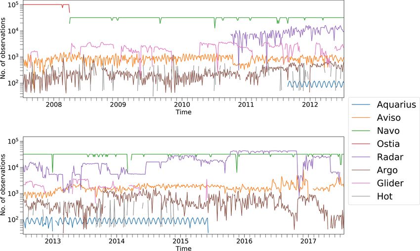
D. Partridge et al.: Hawaiian Island Ocean Forecast System                                                                              199

Figure 2. Composite image of percentage coverage for all radar sites (situated at green dots) when all are operational. Where two sites
overlap the greater value is taken to indicate the level of coverage at each point.

Figure 3. Number of observations used within data assimilation run. Note that there tend to be orders-of-magnitude more satellite or remotely
sensed observations than in situ.

of the instruments, provide a smaller amount of data by an               reduction between the initial and final cost function for each
order of magnitude.                                                      cycle to assess how the assimilation performs over time. Ad-
                                                                         ditionally, the I4D-Var algorithm reports the individual con-
                                                                         tributions by the state variables considered by the data as-
3     Assimilation statistics                                            similation to the total cost function. Hence we can examine
                                                                         the cost function in detail for those observation types that are
In this section we examine the state estimate to quantify the            most critical for its reduction. However, it should be noted
performance during our time period.                                      that for this decomposition we do not distinguish between
                                                                         observation sources.
3.1    Cost function reduction
                                                                            Figure 4 shows the time series of the total reduction and
                                                                         the percentage reduction in the cost function for each of the
I4D-Var minimizes the residuals between the model and ob-
                                                                         variables we observe: sea surface height, temperature, salin-
servations over each 4-day cycle. We calculate the percentage

www.geosci-model-dev.net/12/195/2019/                                                          Geosci. Model Dev., 12, 195–213, 2019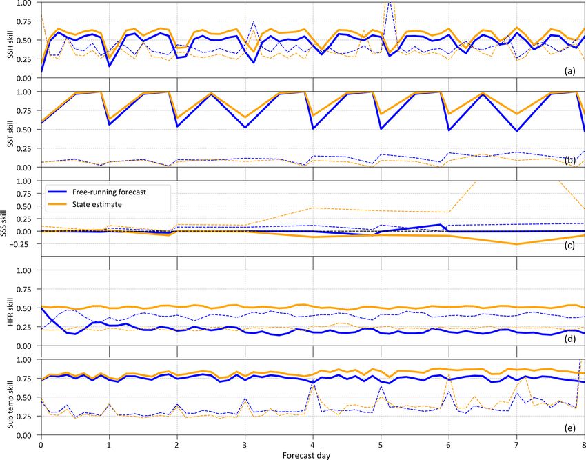
200                                                                   D. Partridge et al.: Hawaiian Island Ocean Forecast System

Figure 4. Time series of percentage reduction in the I4D-Var cost function; in the left column are pre-HFR observations and in the right
column are post-HFR observations, with the mean value given in parentheses. Dashed lines mark the limit of 0, below which there is no
reduction in the cost function for that variable. (a) Total cost function reduction for all observations; (b) sea surface height observations,
(c) temperature observations; (d) salinity observations; (e) HFR observations.

ity, and HFR. A value of 0 means the final cost function is the             The cost function associated with HFR measurements is
same as the initial and no reduction has occurred. The plot is           reduced by 60 % of the initial value, meaning the model is
split into two distinct time periods, before and after the HFR           closer to the HFR observations after the assimilation.
observations, in order to assess changes in the relative con-
tributions of each variable to the overall reduction.                    3.2    Optimality
    The total cost function of all data (Fig. 4a) is on average
halved for each cycle, with an improvement from 49 % of the              Another measure of performance is the theoretical minimum
original value to 55 % when HFR observations are available.              value of the cost function (Jmin ). For a linear system and as-
Looking at the breakdown in Fig. 4b–e, we see that the fi-               suming that the error matrices P and R have been determined
nal cost function associated with the other observed variables           correctly, Jmin is a chi-squared variable whose degrees of
(sea surface height, temperature, and salinity) is reduced by            freedom are given by the number of assimilated observations
a smaller percentage than before HFR was included. Given                 (Nobs ) (Bennett, 2002). The expected value of Jmin is then
that the structure of the cost function is determined by the             given by
type and number of observations, this change in contribution                         Nobs
to the cost function reduction can be expected when adding a             hJmin i =        .                                               (1)
                                                                                      2
large number of HFR measurements to the data assimilation.
    Salinity measurements tend to contribute the least im-               Using above the equation, an optimality value (γ ) can be de-
provement, ranging from 34 % (pre-HFR) to 16 % (post-                    fined:
HFR). Salinity data are the least numerous (Fig. 3) and SSS
fields taken from Aquarius are subject to high noise levels                    2 · Jmin
                                                                         γ=             ,                                                 (2)
(0.2 ppt) and coarse spatial resolution. The mid-2014 drop in                   Nobs
cost function reduction for salinity data coincides with the
                                                                         which
                                                                         √     should reach a value of 1 with a standard deviation of
loss of two Seagliders. After the cessation of Seaglider mis-
                                                                           2/Nobs .
sions salinity data were only available through Aquarius (un-
                                                                           This optimality value provides a simple representation of
til mid-2015) and sporadic Argo profiles.
                                                                         how consistently the error matrices (P and R) are specified,

Geosci. Model Dev., 12, 195–213, 2019                                                         www.geosci-model-dev.net/12/195/2019/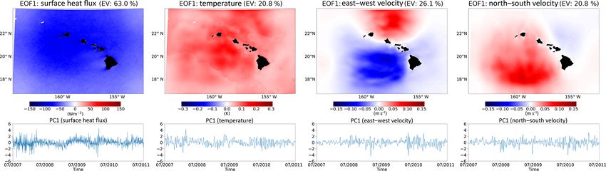
D. Partridge et al.: Hawaiian Island Ocean Forecast System                                                                              201

Figure 5. (a) Gantt chart of remotely sensed observations used in the study. (b) Optimality of I4D-Var data assimilation with the dashed line
representing the theoretical minimum.

since the error covariances normalize the cost function. Fig-            tor Hj ,
ure 5 shows a time series of the calculated optimality value
for the model run, in addition to a timeline of the availabil-           djob = yj − Hj (x b ),                                          (3)
ity of certain observations for reference. Over the full time
period the mean optimality is 0.95. However, there are large             and the difference between x b and the analysis value (x a )
significant deviations over the course of the time period. In            mapped to the observation location,
the pre-HFR period the optimality is low, suggesting that the
error bounds on observations are too wide. Since SST is the              djab = Hj (x a ) − Hj (x b ),                                   (4)
dominant source of observations before HFR, the prescribed
                                                                         one can compute the expected a posteriori background error:
errors associated with SST may be too large.
   Post-HFR, the optimality value increases, suggesting the                          pi
                                                                            b) = 1
                                                                              2     X
errors in this period are underestimated. A large optimality             (σ
                                                                          g
                                                                           i             (Hj (x a ) − Hj (x b ))(yj − Hj (x b )),        (5)
                                                                                 pi j =1
value arises when the cost function is large (i.e., large dif-
ferences between the model and observations). There were
                                                                         where i refers to the observation type and pi is the number
two anomalous cycles in 2011; the first coincides with the
                                                                         of observations of that type.
introduction of a second radar site. From 2012 onwards the
                                                                            Similarly, using the difference between the observation j
optimality value is generally good, if highly variable. The in-
                                                                         and the modeled analysis value (x a ) mapped to the observa-
crease in optimality given the available observations points to
                                                                         tion,
an underestimation of HFR errors or at the least a persistent
difference between the model and HFR observations.                       djoa = yj − Hj (x a ),                                          (6)

                                                                         the expected a posteriori observation error can be calculated:
3.3   Error consistency
                                                                                     pi
                                                                            b) = 1
                                                                              2     X
                                                                         (σ
                                                                          g
                                                                           i             (yj − Hj (x a ))(yj − Hj (x b )).               (7)
The consistency of the assimilation can be assessed by com-                      pi j =1
paring the error matrices P and R specified a priori with the
observation and background error covariances determined a                   For a detailed description of the above diagnostics the
posteriori (Desroziers et al., 2005). Using the difference be-           reader is referred to Desroziers et al. (2005, 2009). If the
tween the observation j (yj ) and the modeled background                 variances in P and R are correctly specified a priori, they
value (x b ) mapped to the observation location by the opera-            will be consistent with the a posteriori errors defined above.

www.geosci-model-dev.net/12/195/2019/                                                             Geosci. Model Dev., 12, 195–213, 2019
202                                                                   D. Partridge et al.: Hawaiian Island Ocean Forecast System

Figure 6. Time series of spatially averaged background (blue) and observation (green) errors, with thick lines showing a priori values and
thin lines the posterior calculated using Eqs. (5) and (7). (a) Sea surface height; (b) sea surface temperature; (c) sea surface salinity; and
(d) HFR.

Figure 6 shows both the a priori and a posteriori errors for                This error consistency analysis supports the conclusions in
the remotely sensed data. The observation a priori values are            Sect. 3.2 that the SST observation errors are overestimated
calculated as the mean error of the observations in each cy-             and HFR values are underestimated. It is worth noting that
cle, while the background a priori values are defined as the             these diagnostics are only estimates used to characterize the
variability of a free-running nonlinear model. If the a poste-           errors and are not the true posterior error.
riori errors are typically larger than the a priori, it implies the
initial errors in P and R are underestimated. Conversely, if
they are smaller the initial errors are likely overestimated.            4    Comparison with observations
   Figure 6a shows that sea surface height errors are consis-
tent, while sea surface temperature, shown in Fig. 6b, sug-              Because I4D-Var relies on the model physics to represent ob-
gests the a priori errors are overestimated. The a priori obser-         servations through time, it should provide better forecasts.
vation errors for NAVO SST observations are defined with a               Time-invariant methods (3D-Var, optimal interpolation) that
minimum error of 0.4 K, but the a posteriori errors are more             perturb the state at single times may better reduce the time-
typically around 0.25 K. The a priori background errors also             fixed cost function, but can add nonphysical structures that
appear overestimated.                                                    generate noisy forecasts.
   Sea surface salinity observation errors (Fig. 6c) are slightly           In this section, we examine the state-estimate solution by
underestimated but generally consistent, as are the back-                comparing the model to observations. For reference, the ob-
ground errors. The HFR observation errors (Fig. 6d) also                 servations are also compared against the forecast starting
appear to be underestimated, with most a priori errors close             from the same time as each state-estimate cycle. The ini-
to the minimum value of 7 cm s−1 . The a posteriori errors               tial and boundary as well as atmospheric and tidal forcings
suggest that a typical value of around 12–15 cm s−1 would                are initially the same for both runs; however, the initial and
be more appropriate. The a priori background errors are rea-             boundary conditions and atmospheric forcing are altered as
sonably consistent with the a posteriori; if anything, they are          part of the state-estimate solution.
slightly overestimated.                                                     For comparing fields we use the root mean squared
                                                                         anomaly (RMSA) and the anomaly correlation coefficient

Geosci. Model Dev., 12, 195–213, 2019                                                         www.geosci-model-dev.net/12/195/2019/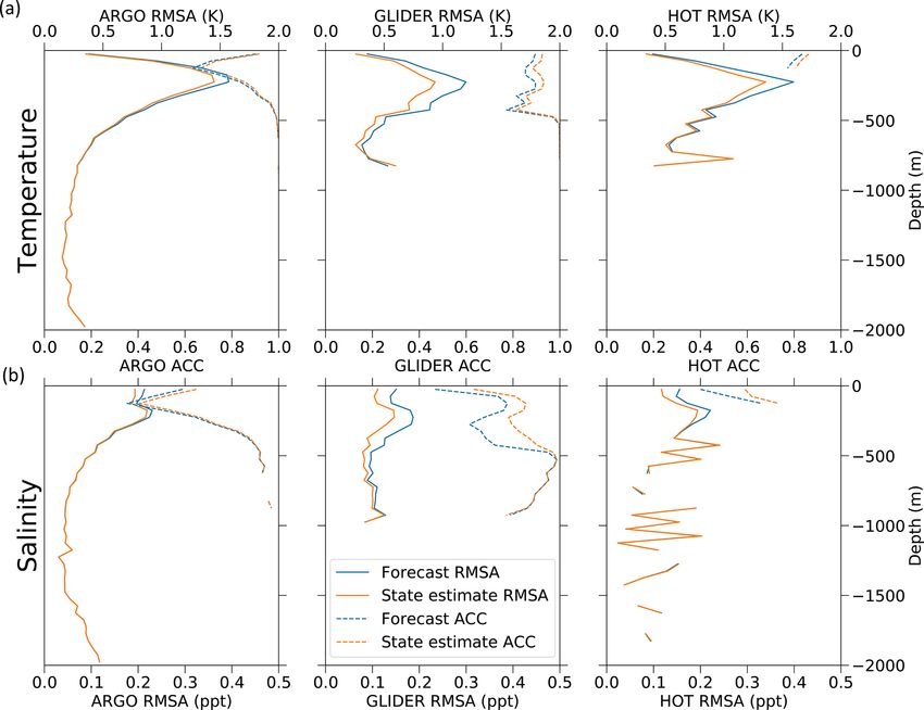
D. Partridge et al.: Hawaiian Island Ocean Forecast System                                                                        203

Figure 7. Time series of root mean squared anomalies (RMSAs) between remotely sensed observations and two model realizations: the state
estimate (orange) and the forecast (blue). (a) Sea surface height; (b) sea surface temperature; (c) sea surface salinity; and (d) HFRs.

(ACC), defined as                                                     nificant impact on the cost function and their representation
                   v                                                  may suffer. We seek to identify these results.
                        N
                   u
                   u1 X
      RMSA(x, y) = t       ((xi − x) − (yi − y))2            (8)      4.1   Remotely sensed observations
                     N i=1
and                                                                   Figure 7 shows the RMSA between the observations and
                        PN                                            the models for each source of remotely observed data. The
                           i=1 (xi− x)(yi − y)                        state-estimate solution reduces the RMSA compared with the
      ACC(x, y) = qP                             ,           (9)
                     N              2 N (y − y)2
                                     P                                forecast by 1.58 cm (17 %), 0.07 K (24 %), 0.01 ppt (3 %),
                        i=1 (xi − x)   i=1  i
                                                                      and 8.39 cm s−1 (37 %) for sea surface height, sea surface
where N is the number of observations and x represents the            temperature, sea surface salinity, and HFR, respectively. In
model values at the same location and time as the obser-              Fig. 7a the RMSA of the state-estimate solution is close to
vations y. The RMSA provides a measure of the residual                the typical observational error of 7 cm, while in Fig. 7b we
between the model and observations, while the ACC deter-              see the RMSA is comfortably less than the 0.4 K represen-
mines the strength of the relationship between the two. We            tative error. Sea surface salinity is only marginally improved
can calculate values for a single spatial point throughout time       by the state-estimate solution, but is slightly over the pre-
or for all spatial points at a single time; however, we require       scribed observational error of 0.2 ppt. The RMSA of the cur-
at least 20 available observation values to get a representa-         rents associated with HFR observations, shown in Fig. 7d, is
tive statistic. The gridded satellite products are ideally suited     improved greatly by the state estimation; however, the mean
to this analysis, while the depth profiles from in situ mea-          value of 14 cm is around double the typical error prescribed
surements are binned into 50 m depth layers to ensure a min-          a priori of 7 cm. As shown in the previous sections, this error
imum number of values. Here it must be noted that our val-            was underestimated.
idation is limited to data that have been employed for the               The ACC is also improved by the state estimate for all
assimilation. The I4D-Var scheme uses the linearized model            variables, as shown in Fig. 8. For sea surface height, temper-
dynamics to produce the covariance between the model and              ature, and salinity the improvement is small due to a signif-
the observations. This allows the model to optimally repre-           icant agreement in the forecast with gains of 0.03, 0.02, and
sent the observations in time and space rather than replicate         0.01, respectively. The improvement in HFR is much more
them. As such, the desire is to use every available observation       significant, with an average correlation improvement from
to constrain this representation. Unlike time-invariant statis-       0.35 to 0.68. As shown in Fig. 8d the free-running forecast
tical methods, we do not withhold any observations because            model can diverge from the observations enough to become
they are sampling the dynamical subspaces of a system of              negatively correlated over a cycle, while the state-estimate
unknown dimension. Since the observations covary in space             solution is consistently positively correlated.
and time, some particular observations may not have a sig-

www.geosci-model-dev.net/12/195/2019/                                                      Geosci. Model Dev., 12, 195–213, 2019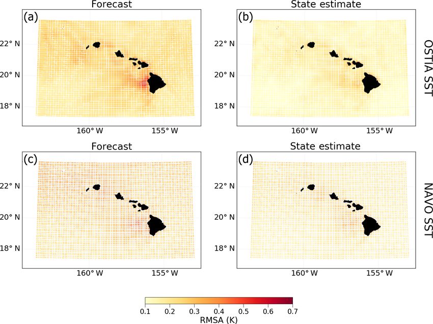
204                                                                 D. Partridge et al.: Hawaiian Island Ocean Forecast System

Figure 8. Time series of anomaly correlation coefficients (ACC) between remotely sensed observations and two model realizations; the state
estimate (orange) and the forecast (blue). (a) Sea surface height; (b) sea surface temperature; (c) sea surface salinity; and (d) HFRs.

Figure 9. Spatial maps of RMSA for SST observation sources for the forecast (a, c) and the state estimate (b, d). (a, b) OSTIA data
(2007–2008); (c, d) NAVO data (2008–2017). The typical error of representativeness is around 0.4 K.

   Figure 9 shows the spatial RMSA between the forecast                (Yang et al., 2008b; Matthews et al., 2012). Even in this peak
and analyses model solutions and the observations for both             area, the state-estimate solution is around the observational
sources of sea surface temperature observations: OSTIA and             error of representativeness of 0.4 K, meaning the model is
NAVO. In both cases there is a clear reduction in the RMSA,            performing well with regards to SST.
with the largest source of error in the areas leeward of the              Both RMSA and ACC between the experiments and HFR
islands, most notably the island of Hawai‘i. This is due to            observations are shown in Fig. 10 for the island of O‘ahu.
higher heat flux variability from a reduction in cloud cover           The RMSA of the free-running forecast is reasonably uni-

Geosci. Model Dev., 12, 195–213, 2019                                                      www.geosci-model-dev.net/12/195/2019/
D. Partridge et al.: Hawaiian Island Ocean Forecast System                                                                              205

Figure 10. Spatial maps of HFR statistics for south O‘ahu for the forecast (a, c) and the state estimate (b, d). (a, b) RMSA; (c, d) ACC.

form across the region covered by the HFR, around 20–                    of improvement from the forecast to the state-estimate solu-
25 cm s−1 , with some varying values around the extent of                tion is consistent with the O‘ahu results shown here.
the radar coverage. The inclusion of HFR observations in the
state-estimate solution leads to significantly reduced values            4.2   Subsurface observations
of 12–15 cm s−1 , a reduction of almost half. The ACC is also
significantly improved from a weak correlation to a consis-              The in situ observation sources are Argo floats, Seagliders,
tently strong positive one.                                              and HOT CTDs, which also show an improvement in the
   As discussed in Souza et al. (2015), there are several                state estimate over the forecast. The subsurface temperature
reasons the model can differ from surface current observa-               RMSA values are reduced by an average of 0.03 K and salin-
tions: the discretization of the model, imperfect stratification,        ity by 0.01 ppt. The average RMSA is within the represen-
differing barotropic-to-baroclinic tide conversion at Kaena              tative errors for both variables at 0.8 K and 0.15 ppt, respec-
Ridge, or mixing parameters that do not capture the real                 tively. However, there are several occasions when the RMSA
baroclinic mixing. This may lead to a different location of              value for a cycle exceeds that limit when there are very few
the currents in the model from those observed by the HFR;                in situ observations available.
however, the model does a good job of reducing these errors                 Figure 11 shows the RMSA and ACC profiles for tem-
(Janeković and Powell, 2012). The HFRs located on the is-               perature and salinity for each source of subsurface observa-
land of Hawai‘i have a smaller coverage region, but the level            tion. For all three sources, the greatest RMSA between the
                                                                         models and observations is along the thermocline where mi-

www.geosci-model-dev.net/12/195/2019/                                                          Geosci. Model Dev., 12, 195–213, 2019
206 D. Partridge et al.: Hawaiian Island Ocean Forecast System
Figure 11. RMSA (solid) and ACC (dashed) profiles of subsurface temperature (a) and salinity (b) for Argo floats, Seagliders, and HOT
CTDs for the forecast (blue) and the state estimate (orange). Data were binned into 50 m intervals.
nor differences in thermocline depth lead to temperature dif- 5 Forecast skill
ferences. The state estimate improves the RMSA in this re-
gion by 10–15 %. The thermocline location is also the source In this section we quantify the model skill by using a skill
of the lowest correlation between the observations and the score evaluated as the improvement against a reference field
model, which is improved by the state estimate by ∼ 5 %. (Murphy, 1988). For the reference, we take the model value
There is a high RMSA for Seagliders at the base of their pro- at the spatial location of each observation at the time of ini-
files (close to 1000 m). In this instance the state estimate does tialization for each 8-day cycle and assume persistence of
not result in an improvement of the forecast. Many of the this value throughout the 8-day cycle (persistence assump-
glider missions operated in the shallow waters off the south tion). The skill score (SS) for the state-estimate analysis and
coast of O‘ahu where processes are at much finer scale than forecast is then defined using the ratios of RMSAs with re-
can be resolved at 4 km resolution. As such, the observational spect to the observations:
representation errors were higher.
For subsurface salinity (Fig. 11b), the improvements made RMSA(x a , y)
SSa = 1 − , (10)
by the state-estimate solution occur almost exclusively above RMSA(x 0 , y)
500 m for Argo floats and HOT CTDs. As with tempera- RMSA(x f , y)
ture the largest improvement is at the top of the thermo- SSf = 1 − , (11)
RMSA(x 0 , y)
cline. There are some low ACC values lower down in the
profile between both models and the observations, but both where the superscripts a, f, and 0 refer to the analysis, free-
the forecast and state estimate perform equally at this depth. running forecast, and persistence, respectively, and y indi-
Seagliders produce the biggest improvement in subsurface cates the observations. Under this measure, a SS of 1 rep-
salinity model performance, with the state-estimate solution resents a perfect fit between the model and observations,
up to 20 % better than the forecast for both RMSA and ACC. while a value of zero indicates where the model and persis-
The peak improvement is at the top of the thermocline, but tence values perform exactly the same. If the model is bet-
there are improvements throughout the profile. ter than persistence, then the skill score will lie in the range
0 < SS < 1 and the degree of improvement over persistence
is determined by how close to 1 the score is. Conversely, a
negative SS means the model is further from the observations
than persistence.
Geosci. Model Dev., 12, 195–213, 2019 www.geosci-model-dev.net/12/195/2019/D. Partridge et al.: Hawaiian Island Ocean Forecast System 207
Figure 12. Mean skill metric for remotely sensed observations as a function of forecast length. Solid lines: skill (see Eqs. 10 and 11); dashed
lines: standard deviation of skill. (a) Sea surface height; (b) sea surface temperature; (c) sea surface salinity; (d) HFRs; and (e) subsurface
temperature.
For this verification we wish to examine the effect of fore- initial conditions are used for persistence values and the di-
cast length on the skill. Starting with the same initial condi- urnal cycle will move ocean temperatures close to this per-
tions as each state-estimate cycle we produce an 8-day fore- sistence value once per day. The state-estimate skill for HFR
cast, the length of two state-estimate cycles. The RMSA is has a consistent value of 0.5 regardless of the forecast day,
calculated every 3 h for each 8-day forecast, the correspond- while the skill of the free-running forecast decreases within
ing state-estimate cycles, and the persistence field from the the first 12 h and is closer to 0.2 for the rest of the forecast pe-
start of the forecast. riod. This decrease in skill is driven by the fact that the radials
Figure 12 shows the mean SS over all cycles for remotely are dominated by the semidiurnal baroclinic and barotropic
sensed observations. For SSH, SST, and HFR, the skill for tides.
both the state-estimation and free-running forecast is positive
throughout, indicating that both models are successful over
persistence in representing those variables. SSS, however, is 6 Analysis of increments
close to zero and slightly negative, meaning the models pro-
vide no better information than persistence. SST values are During each I4D-Var 4-day window, the initial model field
consistently the highest, with a reduction in skill versus per- and time-varying boundary and surface forcings are adjusted
sistence for both models once per day. This is expected as to minimize the residuals. The initial condition increments
form a single record for each cycle, while the boundary and
www.geosci-model-dev.net/12/195/2019/ Geosci. Model Dev., 12, 195–213, 2019208 D. Partridge et al.: Hawaiian Island Ocean Forecast System Figure 13. EOF1 and PC1 of initial condition increments for temperature, east–west velocity, and north–south velocity (all averaged 0– 100 m) and of forcing perturbations applied to surface heat flux. The EOFs were calculated using the routines described in Dawson (2016). surface forcings are perturbed every time they are applied model grid, the number of records, and the computational to the model. The perturbations applied to the boundary ex- resources available the EOF calculation is limited to a 4- hibit only a minor influence on the model (not shown) due year period, with approximately 1500 records. Several dif- to the mean advection speed (≈ 20 cm s−1 ) and sponge layer ferent periods were examined with no significant differences dampening near the boundaries. We focus our analysis on the in the structure of the modes or their percentage of variance increments of the initial conditions and the surface forcing. explained. The time of day does impact the percentage of Because we are analyzing the increments (rather than variance explained by each mode, most notably for surface the state) to the initial conditions and forcing fields, the heat flux for which the effect of diurnal solar heating occurs. mean increment should be zero (unless there is a bias in However, the overall locations and magnitudes of the peaks the model), and we are looking to examine the variability. and troughs as well as the temporal evolution of PCs do not Over the entire reanalysis period, the mean biases between exhibit significant differences for each time of day, so we the model and observations for the different types are temper- present one of the modes for each considered variable. ature (−0.0048 K), salinity (0.0049 ppt), SSH (−7 mm), and The four key surface forcing terms are surface heat flux, HFR (0.06 cm s−1 ). A consistent pattern or principal compo- surface salinity flux, east–west wind stress, and north–south nent may suggest a repeated correction to account for miss- wind stress. Of these, increments in surface salinity flux are ing or misrepresented physics in the model. quite small compared to their initial value, while increments Over the 10-year reanalysis, there are 917 analysis cycles in surface heat flux (10 %–15 % of initial value) and the wind with 16 surface forcing adjustments (four per day) per cy- stresses (15 %–20 % of initial value) are significant. cle. We calculated the empirical orthogonal functions (EOFs) For surface heat flux and near-surface temperature, we ob- (Hannachi, 2004) of the increments applied to the forcing and serve that the EOF1 modes represent 63 % and 20.8 % of the the initial conditions to analyze the dominant spatial patterns variability, respectively, with a consistent sign over the re- of the adjustments. gion (Fig. 13). This mode essentially accounts for the bias For each cycle, the initial perturbation of the primary between our ocean model and the WRF atmospheric model model prognostic variables are examined: sea surface height, used to force the surface. Unfortunately, WRF was not inte- temperature, salinity, east–west velocity, and north–south ve- grated loosely coupled to the ROMS using the ROMS SST locity. With the exception of sea surface height, each variable field; rather, it was run using persistent estimates of daily is averaged over the upper 100 m to cover the mixed layer SST during its integration. It must be noted, however, that the depth in the domain (Matthews et al., 2012). The increments monopole structure of the EOF1 does not represent a con- for salinity and sea surface height as a percentage of the ini- stant offset between ROMS and WRF since the actual per- tial conditions are insignificant (< 1 %), while temperature turbation of surface heat flux and increment applied to near- increments (2–10 %) and the two velocity fields (10–20 %) surface temperature are given by the products of the respec- are significant enough to analyze. tive EOF1 and the PC1. As can be seen in the lower panels The assimilation was configured to optimize the surface of Fig. 13, the temporal evolution of the PC1 for both surface forcing increments every 6 h (to avoid overadjustment). The heat flux and near-surface temperature adjustments is domi- time of day potentially impacts forcing variables, particu- nated by high-frequency, nonphysical variance. larly surface heat flux, so we calculate EOFs on the incre- The EOF1 modes of the near-surface velocity increments ments for each of the four distinct times of day they occur explain 26.1 % and 20.8 % of the variance, respectively. Both (00:00, 06:00, 12:00, 18:00 UTC). Due to the size of the modes exhibit a strong impact south of the main Hawaiian Geosci. Model Dev., 12, 195–213, 2019 www.geosci-model-dev.net/12/195/2019/
D. Partridge et al.: Hawaiian Island Ocean Forecast System                                                                            209

Figure 14. Spatial EOF patterns and principal components (PCs) of wind stress perturbations for the period prior to the assimilation of HFR
measurements (June 2007–September 2010).

Islands. The structure of the wind stress curl in this region           Flament, 2013) (see also Fig. 1). The EOF1 modes of the
results in the spin-up of cyclonic and anticyclonic eddies to           near-surface velocity increments are responsible for adjust-
the north and south of the lee side of each island, respectively        ing the state estimate for the significant eddy activity in the
(Chavanne et al., 2002). As a consequence, a zone of strong             lee of Hawai‘i.
current shear is created between the North Equatorial Cur-                 The EOFs of surface wind stress increments are confined
rent and the Hawaiian Lee Counter Current (Lumpkin and                  to relatively small regions of the model domain (Figs. 14

www.geosci-model-dev.net/12/195/2019/                                                         Geosci. Model Dev., 12, 195–213, 2019
210                                                                D. Partridge et al.: Hawaiian Island Ocean Forecast System

Figure 15. Spatial EOF patterns and principal components (PCs) of wind stress perturbations for the period including the assimilation of
HFR measurements (January 2011–January 2014).

and 15). A significant change occurs after the HFR obser-             portant role as a vorticity source to the ocean (Souza et al.,
vations come online. During the period prior to the availabil-        2015). Hence the adjustment of wind stress in the channels
ity of the HFR data (June 2007–September 2010), the wind              between the islands is critical for a reliable representation of
stress was primarily adjusted in the lee regions where the            ocean conditions. The magnitude and sign of the PCs of the
winds are forced between islands (e.g., Kaiwi, ‘Alenuihāhā          wind stress adjustments for this period are driven by day-
Channels, and to a smaller degree over the Kaua‘i Channel;            to-day variability (Fig. 14, lower panels). Also, the PCs of
Fig. 14). The wind stress curl in these regions plays an im-          the east–west wind stress and north–south wind stress are

Geosci. Model Dev., 12, 195–213, 2019                                                     www.geosci-model-dev.net/12/195/2019/
D. Partridge et al.: Hawaiian Island Ocean Forecast System                                                                      211

largely uncorrelated, aggravating an interpretation of the ad-    increments are concentrated in the region south of O‘ahu.
justments in terms of a larger-scale atmospheric pattern or       The wind stress heavily influences the surface currents and
wind stress curl.                                                 adjustments are mostly made as a consequence to HFR data.
   With the integration of the HFR measurements (Octo-            Additional analysis reveals that wind stress adjustments in
ber 2010), the dominant wind stress increments occur across       the channels between the islands dominated the increments
the shallow region close to the south coast of O‘ahu (Fig. 15).   in the period prior to the radar-based measurements of sur-
The first mode for both east–west and north–south wind            face currents.
stress exhibits a monopole structure adjusting the wind stress       The reanalysis has provided the testing for improvements
uniformly across the area covered by the HFR and its vicin-       to the PacIOOS operational forecast system. The data are be-
ity. The second modes have an east–west dipole structure that     ing used to update the back catalog available to the public
will either increase or decrease the wind stress shear around     at http://www.pacioos.hawaii.edu (last access: 22 December
the HFR region. Similarly to the pre-HFR period, the PCs          2018) and will influence the future results from daily fore-
of the wind stress increments are dominated by day-to-day         casts. Analysis of the I4D-Var increments has provided a
variability and do not represent a physical mode.                 greater understanding of the variability in the region and will
                                                                  provide the basis for a move towards ensemble forecasting in
                                                                  the region.
7   Conclusions

We have presented a 10-year reanalysis of the PacIOOS             Code availability. The specific ROMS Fortran source for this
Hawaiian Island Ocean Forecast System and assessed                package is under the MIT license and is available from
the performance of the state-estimate solution and free-          https://doi.org/10.5281/zenodo.1493617 (Powell et al., 2018).
running forecasts. Using a time-dependent incremental             Model initial conditions and boundary forcing come from the HY-
                                                                  brid Coordinate Ocean Model (http://hycom.org, last access: 22 De-
strong-constraint four-dimensional variational data assimila-
                                                                  cember 2018).
tion (I4D-Var) scheme, we show that the model represents
the observational data well over the time period. The state-
estimate solution reduces the RMSA compared to the fore-
                                                                  Data availability. Atmospheric surface forcing and HF radar ob-
cast by 3 % (salinity) to 37 % (surface velocities). A limi-      servations are distributed through the PacIOOS data portal at
tation of the model–observation comparison is given by the        http://pacioos.hawaii.edu (last access: 22 December 2018). Satel-
fact that in the absence of a sufficient number of independent    lite measurements come from two sources; sea surface tempera-
observations, only assimilated data could be used for the val-    ture and salinity are provided by the Physical Oceanography Dis-
idation.                                                          tributed Active Archive Centre at http://podaac.jpl.nasa.gov (last
   The largest reduction of the cost function of the state-       access: 22 December 2018), and surface height anomalies are pro-
estimate solution occurs when minimizing the residuals to         vided by the Copernicus Marine Environment Monitoring Service
HFR data, with SST also accounting for a significant im-          at http://marine.copernicus.eu (last access: 22 December 2018). In
provement. On average, the assimilation achieves the near-        situ measurements used are available from three sources: Argo mea-
                                                                  surements through the Global Ocean Data Assimilation Experiment
optimal solution; however, the variability is heavily influ-
                                                                  at http://usgodae.org (last access: 22 December 2018), Seaglid-
enced by the HFR observations. The analysis suggests that
                                                                  ers through the School of Ocean and Earth Science and Technol-
the observational errors associated with HFR are too low and      ogy at the University of Hawai‘i at Mānoa at http://hahana.soest.
results could be improved by redefining these errors. This is     hawaii.edu/seagliders (last access: 22 December 2018), and CTDs
supported by the increase in variability and upward trend of      through the Hawai‘i Ocean Time-Series project at http://hahana.
optimality towards the end of the time period during which        soest.hawaii.edu/hot (last access: 22 December 2018). Reanalysis
HFR observations are most numerous.                               output is produced as 3-hourly snapshots of the 3-D field tem-
   The increments made by the reanalysis have revealed that       perature, salinity, and velocities interpolated onto a z grid from
sea surface height and salinity initial conditions are not sig-   the native s grid, as well as the 2-D sea surface height field
nificantly adjusted by the I4D-Var procedure, whereas tem-        for the full time period. These data are archived through the Pa-
perature and velocity account for a significant change from       cIOOS data server at http://oos.soest.hawaii.edu/thredds/idd/ocn_
                                                                  mod_hiig.html?dataset=roms_hiig_reanalysis (last access: 22 De-
the forecast field. For the atmospheric forcing, surface salin-
                                                                  cember 2018).
ity is insignificant, but the adjustments made to surface heat
flux and wind stresses alter the forcings by up to 20 %. This
corresponds to cost function statistics that point to HFR and
                                                                  Author contributions. DP and BSP designed and conducted the re-
temperature as the two dominant observation sources.              analysis simulations. All three authors contributed to the analysis
   The dominant EOF mode for adjustments of surface heat          and interpretation of the model results and to writing the paper.
flux and near-surface temperature exhibits a monopole struc-
ture, indicating a slight bias correction between the ocean
and atmospheric model. The leading modes of wind stress

www.geosci-model-dev.net/12/195/2019/                                                   Geosci. Model Dev., 12, 195–213, 2019
212 D. Partridge et al.: Hawaiian Island Ocean Forecast System
Competing interests. The authors declare that they have no conflict verse model, J. Geophys. Res.-Oceans, 99, 24821–24852,
of interest. https://doi.org/10.1029/94JC01894, 1994.
Flather, R.: A Tidal Model of the Northwest European Continental
Shelf, Mem. Soc. R. Sci. Liege, 10, 141–164, 1976.
Acknowledgements. The authors would like to thank the GODAE Hannachi, A.: A Primer for EOF Analysis of Climate Data, Tech.
for hosting the Argo observations and the HOT project for CTD and rep., Department of Meteorology, University of Reading, 2004.
Seaglider data. The authors would also like to thank Yi-Leng Chen HMRG: Hawaii Mapping Research Group, SOEST, available at:
of the University of Hawai‘i Department of Meteorology for the http://www.soest.hawaii.edu/HMRG/multibeam/index.php (last
atmospheric model data MM5 and WRF. The authors are grateful access: 13 April 2018), 2017.
to two anonymous reviewers and the editor for helping improve this Janeković, I. and Powell, B. S.: Analysis of imposing tidal dynam-
paper. This work was supported by PacIOOS (http://pacioos.org, ics to nested numerical models, Cont. Shelf Res., 34, 30–40,
last access: 22 December 2018), which is a part of the US https://doi.org/10.1016/j.csr.2011.11.017, 2012.
Integrated Ocean Observing System (IOOS® ), funded in part by Janeković, I., Powell, B. S., Matthews, D., McManus, M. A., and
National Oceanic and Atmospheric Administration (NOAA) award Sevadjian, J.: 4D-Var data assimilation in a nested, coastal ocean
no. NA16NOS0120024. This is SOEST publication no. 10525. model: A Hawaiian case study, J. Geophys. Res.-Oceans, 118,
5022–5035, https://doi.org/10.1002/jgrc.20389, 2013.
Edited by: Steven Phipps Kerry, C., Powell, B., Roughan, M., and Oke, P.: Development and
Reviewed by: two anonymous referees evaluation of a high-resolution reanalysis of the East Australian
Current region using the Regional Ocean Modelling System
(ROMS 3.4) and Incremental Strong-Constraint 4-Dimensional
References Variational (IS4D-Var) data assimilation, Geosci. Model Dev., 9,
3779–3801, https://doi.org/10.5194/gmd-9-3779-2016, 2016.
Bennett, A.: Inverse Modeling of the Ocean Kistler, R., Kalnay, E., Collins, W., Saha, S., White, G., Woollen,
and Atmosphere, Cambridge University Press, J., Chelliah, M., Ebisuzaki, W., Kanamitsu, M., Kousky, V., van
https://doi.org/10.1017/CBO9780511535895, 2002. den Dool, H., Jenne, R., and Fiorino, M.: The NCEP–NCAR 50-
Broquet, G., Edwards, C., Moore, A., Powell, B., Veneziani, M., and year reanalysis: monthly means CD-ROM and documentation,
Doyle, J.: Application of 4D-Variational data assimilation to the B. Am. Meteorol. Soc., 82, 247–268, 2001.
California Current System, Dynam. Atmos. Oceans, 48, 69–92, Lumpkin, R. and Flament, P.: Extent and Energetics of the
https://doi.org/10.1016/j.dynatmoce.2009.03.001, 2009. Hawaiian Lee Countercurrent, Oceanography, 26, 58–65,
Chapman, D. C.: Numerical Treatment of Cross-Shelf Open https://doi.org/10.5670/oceanog.2013.05, 2013.
Boundaries in a Barotropic Coastal Ocean Model, J. Phys. Matthews, D., Powell, B. S., and Milliff, R.: Domi-
Oceanogr., 15, 1060–1075, https://doi.org/10.1175/1520- nant spatial variability scales from observations around
0485(1985)0152.0.CO;2, 1985. the Hawaiian Islands, Deep-Sea Res., 58, 979–987,
Chassignet, E. P., Hurlburt, H. E., Smedstad, O. M., Halli- https://doi.org/10.1016/j.dsr.2011.07.004, 2011.
well, G. R., Hogan, P. J., Wallcraft, A. J., Baraille, R., Matthews, D., Powell, B. S., and Janeković, I.: Analy-
and Bleck, R.: The HYCOM (HYbrid Coordinate Ocean sis of four-dimensional variational state estimation of the
Model) data assimilative system, J. Marine Syst., 65, 60–83, Hawaiian waters, J. Geophys. Res.-Oceans, 117, C03013,
https://doi.org/10.1016/j.jmarsys.2005.09.016,2007. https://doi.org/10.1029/2011JC007575, 2012.
Chavanne, C., Flament, P., Lumpkin, R., Dousset, B., and Bentamy, Milliff, R. F., Morzel, J., Chelton, D. B., and Freilich, M. H.: Wind
A.: Scatterometer observations of wind variations induced by stress curl and wind stress divergence biases from rain effects on
oceanic islands: Implications for wind-driven ocean circulation, QSCAT surface wind retrievals, J. Atmos. Ocean. Technol., 21,
Can. J. Remote Sens., 28, 466–474, https://doi.org/10.5589/m02- 1216–1231, 2004.
047, 2002. Moore, A. M., Arango, H. G., Lorenzo, E. D., Cornuelle, B. D.,
Courtier, P., Thépaut, J.-N., and Hollingsworth, A.: A strategy Miller, A. J., and Neilson, D. J.: A comprehensive ocean pre-
for operational implementation of 4D-Var, using an incremen- diction and analysis system based on the tangent linear and ad-
tal approach, Q. J. Roy. Meteorol. Soc., 120, 1367–1387, joint of a regional ocean model, Ocean Model., 7, 227–258,
https://doi.org/10.1002/qj.49712051912, 1994. https://doi.org/10.1016/j.ocemod.2003.11.001, 2004.
Dawson, J.: eofs: A Library for EOF Analysis of Meteorological, Moore, A. M., Arango, H. G., Broquet, G., Edwards, C.,
Oceanographic, and Climate Data, J. Open Research Softw., 4, Veneziani, M., Powell, B., Foley, D., Doyle, J. D., Costa,
e14, https://doi.org/10.5334/jors.122, 2016. D., and Robinson, P.: The Regional Ocean Modeling Sys-
Desroziers, G., Berre, L., Chapnik, B., and Poli, P.: Diagnosis tem (ROMS) 4-dimensional variational data assimilation
of observation, background and analysis error statistics in ob- systems: Part II – Performance and application to the
servation space., Q. J. Roy. Meteorol. Soc., 131, 3385–3396, California Current System, Prog. Oceanogr., 91, 50–73,
https://doi.org/10.1256/qj.05.108, 2005. https://doi.org/10.1016/j.pocean.2011.05.003, 2011a.
Desroziers, G., Berre, L., Chabot, V., and Chapnik, Moore, A. M., Arango, H. G., Broquet, G., Edwards, C.,
B.: A Posteriori Diagnostics in an Ensemble of Per- Veneziani, M., Powell, B., Foley, D., Doyle, J. D., Costa,
turbed Analyses, Mon. Weather Rev., 137, 3420–3436, D., and Robinson, P.: The Regional Ocean Modeling System
https://doi.org/10.1175/2009MWR2778.1, 2009. (ROMS) 4-dimensional variational data assimilation systems:
Egbert, G. D., Bennett, A. F., and Foreman, M. G. G.: Part III – Observation impact and observation sensitivity in
TOPEX/POSEIDON tides estimated using a global in-
Geosci. Model Dev., 12, 195–213, 2019 www.geosci-model-dev.net/12/195/2019/You can also read