COMPARISON OF POPULAR DATA PROCESSING SYSTEMS - KTH THESIS REPORT KAMIL NASR - DIVA
←
→
Page content transcription
If your browser does not render page correctly, please read the page content below
DEGREE PROJECT IN COMPUTER SCIENCE AND ENGINEERING,
SECOND CYCLE, 30 CREDITS
STOCKHOLM, SWEDEN 2021

Comparison of
Popular Data
Processing Systems
KTH Thesis Report

Kamil Nasr

 KTH ROYAL INSTITUTE OF TECHNOLOGY
 ELECTRICAL ENGINEERING AND COMPUTER SCIENCE
Author
Kamil Nasr
Communication Systems Design
KTH Royal Institute of Technology

Examiner and Supervisor
Slimane Ben Slimane
Division of Communication Systems
KTH Royal Institute of Technology

                                    ii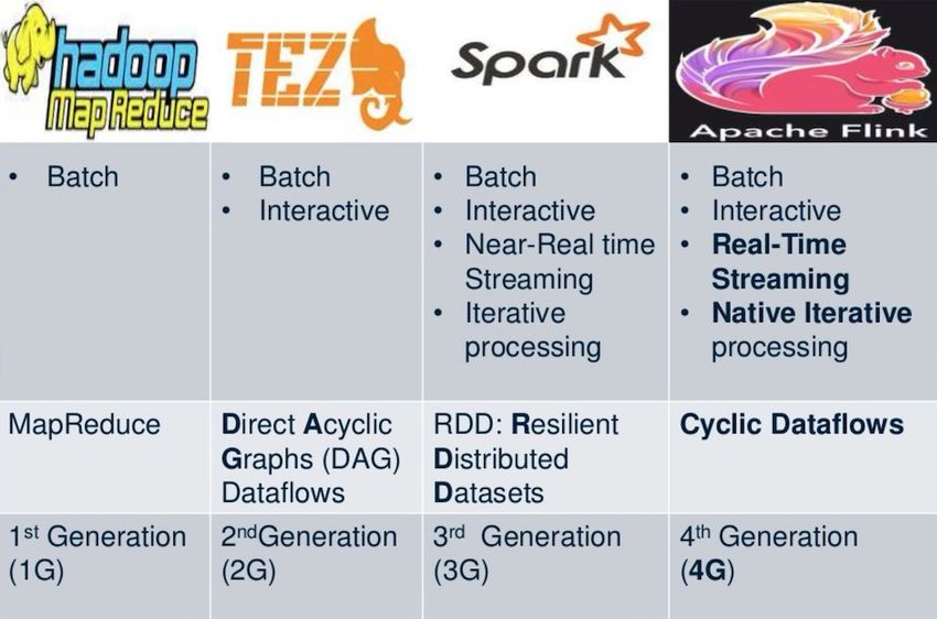
Abstract
Data processing is generally defined as the collection and transformation of data to
extract meaningful information. Data processing involves a multitude of processes
such as validation, sorting summarization, aggregation to name a few. Many analytics
engines exit today for largescale data processing, namely Apache Spark, Apache
Flink and Apache Beam. Each one of these engines have their own advantages and
drawbacks. In this thesis report, we used all three of these engines to process data
from the Carbon Monoxide Daily Summary Dataset to determine the emission levels
per area and unit of time. Then, we compared the performance of these 3 engines
using different metrics. The results showed that Apache Beam, while offered greater
convenience when writing programs, was slower than Apache Flink and Apache Spark.
Spark Runner in Beam was the fastest runner and Apache Spark was the fastest data
processing framework overall.
Keywords
Apache Spark, Apache Flink, Apache Beam, Spark Runner, Flink Runner, Direct
Runner, Big Data Analytics, Data Processing Systems, Benchmarking, Kaggle
iii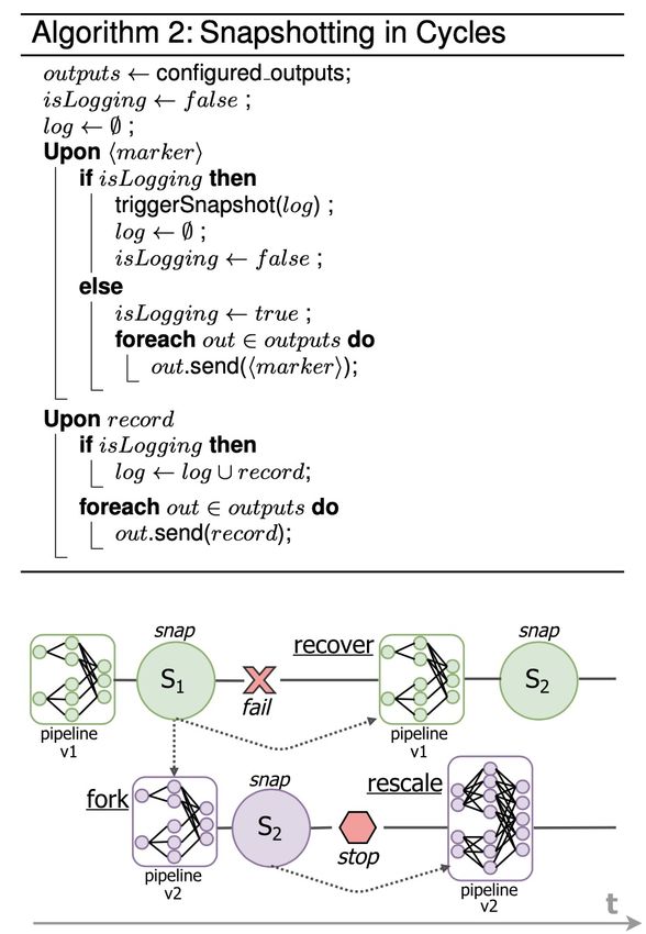
Abstract

Databehandling definieras generellt som insamling och omvandling av data för att
extrahera meningsfull information. Databehandling involverar en mängd processer
som validering, sorteringssammanfattning, aggregering för att nämna några. Många
analysmotorer lämnar idag för storskalig databehandling, nämligen Apache Spark,
Apache Flink och Apache Beam. Var och en av dessa motorer har sina egna fördelar
och nackdelar. I den här avhandlingsrapporten använde vi alla dessa tre motorer för att
bearbeta data från kolmonoxidens dagliga sammanfattningsdataset för att bestämma
utsläppsnivåerna per område och tidsenhet. Sedan jämförde vi prestandan hos dessa
3 motorer med olika mått. Resultaten visade att Apache Beam, även om det erbjuds
större bekvämlighet när man skriver program, var långsammare än Apache Flink och
Apache Spark. Spark Runner in Beam var den snabbaste löparen och Apache Spark
var den snabbaste databehandlingsramen totalt.

Nyckelord

Apache Spark, Apache Flink, Apache Beam, Spark Runner, Flink Runner, Direct
Runner, Big Data Analytics, Data Processing Systems, Benchmarking, Kaggle

                                                                                     iv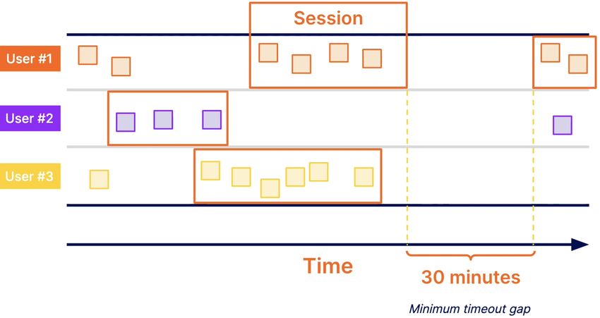
Acknowledgements

I would like to thank my professor Slimane Ben Slimane for his constant help and
support during the writing of this thesis report, as well as all my other professors at
KTH who made this possible.

                                                                                     v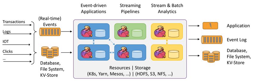
Contents

1 Introduction                                                                           1
  1.1 Motivation . . . . . . . . . . . . . . . . . . . . . . . . . . . . . . . . . . .    1
  1.2 Problem . . . . . . . . . . . . . . . . . . . . . . . . . . . . . . . . . . . .     2
  1.3 Purpose . . . . . . . . . . . . . . . . . . . . . . . . . . . . . . . . . . . .     2
  1.4 Goal . . . . . . . . . . . . . . . . . . . . . . . . . . . . . . . . . . . . . .    3
  1.5 Benefits, Ethics and Sustainability . . . . . . . . . . . . . . . . . . . . .       3
  1.6 Delimitations . . . . . . . . . . . . . . . . . . . . . . . . . . . . . . . . .     4
  1.7 Outline . . . . . . . . . . . . . . . . . . . . . . . . . . . . . . . . . . . .     4

2 Background                                                                             5
  2.1 Data Processing Systems . . . . . . . . . . . . . . . . . . . . . . . . . .         5
  2.2 Kaggle . . . . . . . . . . . . . . . . . . . . . . . . . . . . . . . . . . . . .    7
  2.3 Batch and Stream processing . . . . . . . . . . . . . . . . . . . . . . . .         8
       2.3.1 Batch processing . . . . . . . . . . . . . . . . . . . . . . . . . .         8
       2.3.2 Stream processing . . . . . . . . . . . . . . . . . . . . . . . . . .        9
  2.4 Apache Beam . . . . . . . . . . . . . . . . . . . . . . . . . . . . . . . .        11
       2.4.1 Overview . . . . . . . . . . . . . . . . . . . . . . . . . . . . . . .      11
       2.4.2 Windowing . . . . . . . . . . . . . . . . . . . . . . . . . . . . . .       13
       2.4.3 Event time and processing time . . . . . . . . . . . . . . . . . .          16
       2.4.4 Triggers . . . . . . . . . . . . . . . . . . . . . . . . . . . . . . . .    16
       2.4.5 Programming model . . . . . . . . . . . . . . . . . . . . . . . . .         16
  2.5 Apache Spark . . . . . . . . . . . . . . . . . . . . . . . . . . . . . . . .       19
       2.5.1 Overview . . . . . . . . . . . . . . . . . . . . . . . . . . . . . . .      19
       2.5.2 Apache Spark stack . . . . . . . . . . . . . . . . . . . . . . . . .        21
  2.6 Apache Flink . . . . . . . . . . . . . . . . . . . . . . . . . . . . . . . . .     24
       2.6.1 Overview . . . . . . . . . . . . . . . . . . . . . . . . . . . . . . .      24

                                                                                         vi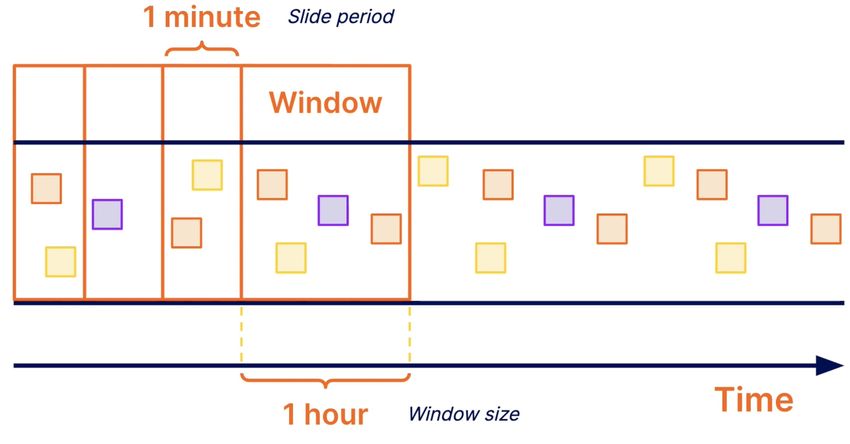
CONTENTS

       2.6.2 Architecture . . . . . . . . . . . . . . . . . . . . . . . . . . . . .        24

3 Related Work                                                                             29
  3.1 Data Stream Processing Systems . . . . . . . . . . . . . . . . . . . . .             29
  3.2 Languages . . . . . . . . . . . . . . . . . . . . . . . . . . . . . . . . . .        34
  3.3 Benchmarks . . . . . . . . . . . . . . . . . . . . . . . . . . . . . . . . .         35
  3.4 Comparisons . . . . . . . . . . . . . . . . . . . . . . . . . . . . . . . . .        36

4 System Design and Implementation                                                         39
  4.1 System Design . . . . . . . . . . . . . . . . . . . . . . . . . . . . . . . .        39
       4.1.1 Data set . . . . . . . . . . . . . . . . . . . . . . . . . . . . . . . .      39
       4.1.2 Queries . . . . . . . . . . . . . . . . . . . . . . . . . . . . . . . .       39
  4.2 Implementation . . . . . . . . . . . . . . . . . . . . . . . . . . . . . . . .       40
       4.2.1 Apache Beam . . . . . . . . . . . . . . . . . . . . . . . . . . . .           40
       4.2.2 Apache Spark in Batch . . . . . . . . . . . . . . . . . . . . . . .           43
       4.2.3 Apache Spark in Stream . . . . . . . . . . . . . . . . . . . . . .            48
       4.2.4 Apache Flink in Batch . . . . . . . . . . . . . . . . . . . . . . . .         50
       4.2.5 Apache Flink in Stream . . . . . . . . . . . . . . . . . . . . . . .          53

5 Results and Evaluation                                                                   57
  5.1 Apache Beam . . . . . . . . . . . . . . . . . . . . . . . . . . . . . . . .          57
       5.1.1 Spark Runner . . . . . . . . . . . . . . . . . . . . . . . . . . . .          57
       5.1.2 Flink Runner . . . . . . . . . . . . . . . . . . . . . . . . . . . . .        58
       5.1.3 Direct Runner . . . . . . . . . . . . . . . . . . . . . . . . . . . .         58
  5.2 Apache Spark . . . . . . . . . . . . . . . . . . . . . . . . . . . . . . . .         59
  5.3 Apache Flink . . . . . . . . . . . . . . . . . . . . . . . . . . . . . . . . .       60
  5.4 Performance Comparison . . . . . . . . . . . . . . . . . . . . . . . . . .           61
       5.4.1 Spark Runner vs Flink Runner vs Direct Runner . . . . . . . . .               61
       5.4.2 Apache Spark vs Spark Runner . . . . . . . . . . . . . . . . . .              62
       5.4.3 Apache Flink vs Flink Runner . . . . . . . . . . . . . . . . . . . .          63
       5.4.4 Apache Spark vs Apache Flink . . . . . . . . . . . . . . . . . . .            64
  5.5 Evaluation     . . . . . . . . . . . . . . . . . . . . . . . . . . . . . . . . . .   65

6 Conclusions and Future Work                                                              66

References                                                                                 68

                                                                                           vii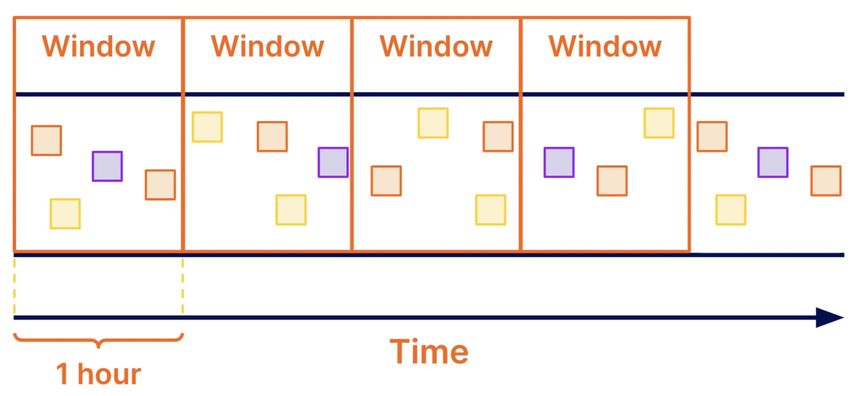
List of Figures
2.1.1 Generations of Big Data Analytics [57] . . . . . . . . . . . . . . . . . . . 5
2.1.2 Data pipeline evolution [67] . . . . . . . . . . . . . . . . . . . . . . . . 6
2.2.1 Kaggle [42] . . . . . . . . . . . . . . . . . . . . . . . . . . . . . . . . . . 7
2.3.1 Batch vs Stream Processing [20] . . . . . . . . . . . . . . . . . . . . . . 8
2.3.2Processing Data Using MapReduce [20] . . . . . . . . . . . . . . . . . . 9
2.3.3Real Time Processing in Spark [20] . . . . . . . . . . . . . . . . . . . . 10
2.4.1 Apache Beam [48] . . . . . . . . . . . . . . . . . . . . . . . . . . . . . . 11
2.4.2The tradeoff between correctness, latency and cost in parallel
processing [5] . . . . . . . . . . . . . . . . . . . . . . . . . . . . . . . . 12
2.4.3Overview of Apache Beam [5] . . . . . . . . . . . . . . . . . . . . . . . . 13
2.4.4Windowing [5] . . . . . . . . . . . . . . . . . . . . . . . . . . . . . . . . 13
2.4.5 Fixed Windows [5] . . . . . . . . . . . . . . . . . . . . . . . . . . . . . . 14
2.4.6Sliding Windows [5] . . . . . . . . . . . . . . . . . . . . . . . . . . . . . 14
2.4.7 Session Windows [5] . . . . . . . . . . . . . . . . . . . . . . . . . . . . . 15
2.4.8Common Windowing Patterns [3] . . . . . . . . . . . . . . . . . . . . . 15
2.4.9Apache Beam programming model [40] . . . . . . . . . . . . . . . . . . 16
2.5.1 Apache Spark [11] . . . . . . . . . . . . . . . . . . . . . . . . . . . . . . 19
2.5.2 Architecture of Apache Spark in Cluster Mode [12] . . . . . . . . . . . . 20
2.5.3 Highlevel architecture of Apache Spark stack [60] . . . . . . . . . . . . 21
2.6.1 Apache Flink [6] . . . . . . . . . . . . . . . . . . . . . . . . . . . . . . . 24
2.6.2Apache Flink Runtime Architecture [24] [35] [36] . . . . . . . . . . . . 24
2.6.3Apache Flink Ecosystem [7] . . . . . . . . . . . . . . . . . . . . . . . . . 25
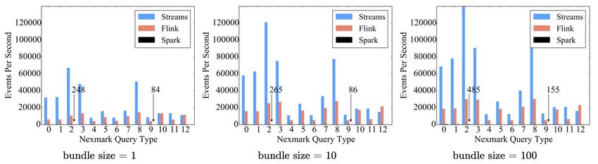
3.1.1 IBM Nexmark Benchmark Evaluation [44] . . . . . . . . . . . . . . . . 29
3.1.2 Datalake in Google Cloud Dataflow [27] . . . . . . . . . . . . . . . . . . 30
3.1.3 Input data goes through MillWheel computations. An external anomaly
notification system consumes the output [2] . . . . . . . . . . . . . . . 30
viii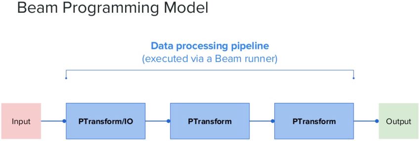
LIST OF FIGURES

  3.1.5 STREAM Query plans [14] . . . . . . . . . . . . . . . . . . . . . . . . .        31
  3.1.4 Simplified Input Data Stream Management System [14] . . . . . . . . .            31
  3.1.6 Apache Calcite architecture and interaction [18] . . . . . . . . . . . . .       32
  3.1.7 Snapshot Algorithm [23] . . . . . . . . . . . . . . . . . . . . . . . . . .      32
  3.1.8 Apache Samza [9] . . . . . . . . . . . . . . . . . . . . . . . . . . . . . .     33
  3.1.9 Heron [55] . . . . . . . . . . . . . . . . . . . . . . . . . . . . . . . . . .   34
  3.1.10Storm High Level Architecture [68] . . . . . . . . . . . . . . . . . . . .       34
  3.2.1 Oracle CEP Architecture [56] . . . . . . . . . . . . . . . . . . . . . . . .     35
  3.4.1 Word count comparison between spark and flink [49] . . . . . . . . . .           37
  3.4.2Throughput results in function of the task parallelism [45] . . . . . . .         37
  3.4.3Average Execution Times in s [36] . . . . . . . . . . . . . . . . . . . . .       38

                                                                                         ix
Chapter 1
Introduction
The world of Big Data is at a massive expansion. People are generating a huge amount
of data everyday through many means, such as online shopping, communications,
media consumption, etc. Data, in order to be of value, needs to be operated on, sorted,
and refined.
In order to do that, many analytics engines, also called data stream processing systems
(DSPSs), exist today, namely Apache Spark, Apache Flink and Apache Beam. Even
though Beam could be better described as an abstraction layer, it still consists of
many runners, such as Spark Runner, Flink Runner and Direct Runner. Each of these
engines have the ability to operate on data whether it is in streaming form or batch
form. Although these engines have quite a bit of similarities, they all have advantages
and drawbacks, depending on the use case.
The idea behind Apache Beam is to give developers the ability to write one code and
choose the appropriate runner. In theory, this is supposed to offer a great deal of
flexibility without the need to rewrite code for different engines.
1.1 Motivation
Studying and comparing different engines can give us a lot of insight on when it is ideal
to use each one of them, as well as the potential sacrifices compared with the gains of
using another. Such knowledge can be of great use for any group of people wanting
to operate and handle large volumes of data, because with the huge portions of time
dedicated to writing appropriate code, as well as the seemingly never ending increases
1CHAPTER 1. INTRODUCTION
in data size, any potential optimization on the programming side or performance side
can be crucial.
1.2 Problem
The need to process evergrowing amounts of data has dictated the creation of data
processing systems or frameworks. However, changing between these frameworks
isn’t guaranteed to be smooth. Adapting a new system can be quite challenging for
most developers, especially when each system uses its own APIs.
Although Apache beam has been created with the premise of a unified model where one
code can be written in Java, Scala or Go, and ran on a multitude of execution engines,
the shift might not be justified with the increase in convenience but with huge potential
drawbacks in performance and execution times.
Even though this balance can only be struck by the developers themselves, it is
important to grasp the potential limitations and opportunities of each framework.
Not only that, but even within Beam itself, which execution engine or runner
is faster, and in which context can have tremendous importance, because the
performance differences between Apache Spark and Apache Flink aren’t guaranteed
to be transferred to Flink Runner and Spark Runner within Apache Beam.
This leads us to four research questions:
• ”How does the performance of Apache Spark compare with that of Apache Flink?”
• ”How does the performance of Spark Runner compare with that of Flink Runner
and Direct Runner?”
• ”How does the Performance of Flink Runner compare with that of Flink?”
• ”How does the performance of Spark Runner compare with that of Spark?”
1.3 Purpose
This thesis report plans on addressing these questions, with the hope of providing some
insight on whether the increase in convenience offered by Beam is at a net win or loss,
depending on the context. Regardless of that, understanding the different performance
2CHAPTER 1. INTRODUCTION
variations in Apache Spark and Apache Flink should give future developers an idea
on which framework or engine best suits their needs before getting stuck with one
framework with the possible challenge of switching to another.
Using the Carbon Monoxide Daily Summary dataset gives us the unique opportunity
to run these different inquiries on data that allows us to get valuable information about
the environmental impact and changes in Carbon Monoxide levels.
All of the above hopefully results in a step forward towards having more efficient and
effective data processing.
1.4 Goal
The goal of this thesis is to sort many different data fields in the very large Carbon
Monoxide Daily Summary dataset using a multitude of data processing engines and
frameworks and appropriate queries in order to determine which ones are faster and
in which scenarios.
1.5 Benefits, Ethics and Sustainability
The main beneficiaries from this project thesis are the companies and developers who
have an interest in using data processing frameworks in their work. This type of
research should hopefully give them an insight on which technologies better suit them
and in which context.
It will also facilitate the choice of changing frameworks based on the priorities they give
to performance versus convenience. Other than that, the Carbon Monoxide emission
results that are sorted in this experiment should give people who are interested in this
cause as well as people who are in charge of decisions affecting the changes in these
metrics some valuable insights on the Carbon Monoxide changes.
When it comes to the ethics and sustainability aspects of this project, no major concerns
are present. The Carbon Monoxide Daily Summary dataset is publicly available on the
Kaggle website, and all data processing frameworks and tools that were used are open
source software.
3CHAPTER 1. INTRODUCTION
1.6 Delimitations
The main delimitations of this project would be that the different results and metrics
that we gather from a certain dataset, even though might offer valuable insights
on the performance differences of all the data processing frameworks used, can not
necessarily be generalized to all datasets.
Other than that, the results and metrics might potentially be different on other
machines and for different versions of the data processing systems.
1.7 Outline
The report is structured in the following way:
First, in Chapter 2, we present and discuss in detail all the technologies and tools
used in this project in order to give the reader better understanding of the rest of the
report.
In Chapter 3, we talk about related work that might add more context to the work done
in this project.
Chapter 4 presents the system design and discusses in detail the experiment
done.
Chapter 5 presents the different results gathered which should help us answer the
research questions.
The last chapter, which is Chapter 6, gives a conclusion to the report and provides some
insight on future work.
4Chapter 2
Background
The aim of this section is to give more information on the different tools and
technologies used in this project. The world of Big Data is an evergrowing world. With
that comes many opportunities but a lot of complexity as well. We hope the reader will
have an easier time understanding the experiments and results of this project after
going through this section.
2.1 Data Processing Systems
Big data processing has evolved around the years and can be generally divided into four
generations, as shown in fig 2.1.1.
Figure 2.1.1: Generations of Big Data Analytics [57]
5CHAPTER 2. BACKGROUND
First generation
The firstgeneration data processing system is Apache Hadoop [8], which primarily
focused on batch data. It also introduced the concepts of Map and Reduce, and
thus provided an opensource implementation of MapReduce [28]. Apache Hadoop
offered many advantages, but its biggest limitation was the involvement of many disk
operations.
Second generation
The second generation data processing systems included slight improvements over
first generation systems. One of the most popular second generation systems is
Tez. Tez introduced interactive programming in addition to batch processing [64]
[19].
Third generation
Apache Spark [10] is the most famous third generation data processing system.
It is considered as a unified model for both stream and batch processing. The
concept of Resilient Distributed Dataset, or RDD, is at the core of Apache Spark
[83]. Machine learning is possible with Apache Spark as it offers support for iterative
processing.
One of the advantages of Apache Spark is that is supports inmemory computation as
well as processing optimization. Spark applications can be written in Java, R, Python
and Scala.
Figure 2.1.2: Data pipeline evolution [67]
6CHAPTER 2. BACKGROUND
Fourth generation
Apache Flink [6] is basically the fourth generation data processing system. Unlike
many other frameworks, Flink supports realtime stream processing. It also supports
both batch and stream processing thanks to the DataSet and DataStream core APIs.
Other supported APIs include SQL as well as the Table API.
Flink also handles stateful stream processing and iterative processing computations.
It can also efficiently handle the challenges of Fault tolerance and scalable state
management [22] [64].
2.2 Kaggle
Figure 2.2.1: Kaggle [42]
Kaggle.com is a very famous website for data scientists and engineers. It gives them
access to huge volume of datasets. It also hosts frequent competitions and challenges
for anyone to join. It even gives prizes for winners.
The Carbon Monoxide Daily Summary dataset that was used to conduct the
experiments in this project was found on Kaggle. It was published by the US
Environmental Protection Agency and contains a summary of daily CO levels of 1990
to 2017.
What is interesting about Kaggle is that it has been called the “AirBnB for Data
Scientists”. It has around half a million active users from over 190 countries. It was
acquired by Google in 2017. What is also important about Kaggle is that it aims to give
7CHAPTER 2. BACKGROUND
data scientists, who don’t often get the chance to practice on real data at least before
joining a company, the opportunity to get some practice on the datasets available on the
platform in different ways including the organized competitions and challenges.
2.3 Batch and Stream processing
In the world of Big Data and Data Analytics, batch data processing and stream data
processing [20] are very important concepts. It is crucial to understand the distinction
between the two principles. Generally speaking, in batch processing, data is collected
first and then processed, whereas stream processing is real time, meaning data is sent
into the analytics tool piecebypiece. Let’s discuss the two concepts in more detail and
give a few examples and use cases for each one of them.
Figure 2.3.1: Batch vs Stream Processing [20]
2.3.1 Batch processing
Batch processing is ideal when we are dealing with relatively large quantities of data,
and/or when the sources of this data are old or legacy systems that aren’t compatible
with stream data processing. For example, mainframe [81] data is processed in batch
by default. It would be quite timely and inconvenient to use mainframe data with newer
analytics environments, thus the challenge in turning it into streaming data.
Figure 2.3.1 shows how Hadoop MapReduce, a popular batch processing framework,
processes data.
8CHAPTER 2. BACKGROUND
Figure 2.3.2: Processing Data Using MapReduce [20]
Batch processing usually shines in scenarios where realtime analytics aren’t necessary,
as well as in those where the ability to process large amounts of data is more important
than the speed of processing said data (slower results for the analytics are acceptable)
[20]. Examples of batch processing use cases include:
• Bills
• Customer orders
• Payroll
2.3.2 Stream processing
If we require analytics results in real time, then stream processing is the only way to go.
The moment the data is generated, it is fed into the analytics tools using data streams.
This allows us to get results that are almost instant. Stream processing can be useful
in fraud detection, because it allows real time detection of anomalies.
The latency in stream processing is usually in seconds or milliseconds, and this is
possible due to the fact that in stream processing data is analyzed before it hits the
disk [20].
Figure 2.3.2 explains how real time processing works in a tool such as Apache
Spark.
9CHAPTER 2. BACKGROUND
Figure 2.3.3: Real Time Processing in Spark [20]
Examples of batch processing use cases include:
• Fraud detection
• Log monitoring
• Customer behavior analysis
• Analyzing social media sentiment
Batch vs Stream processing
The type of data that the data engineer or scientist is dealing with determines to a
large extent whether batch or stream processing is more optimal. However, it is
possible to transform batch data into stream data in order to leverage real time analytic
results. This might provide the chance of being able to react faster to opportunities or
challenges in cases where time constraints apply.
Batch processing Stream processing
Data is collected over a certain Data is collected
period of time continuously
Data is processed only after it’s all Data is processed live,
collected piecebypiece
It can take a long time and is more It’s fast and more suitable
suitable for a large quantity of data for data that needs
with low time restriction immediate processing
10CHAPTER 2. BACKGROUND
2.4 Apache Beam
2.4.1 Overview
Figure 2.4.1: Apache Beam [48]
Apache Beam is a parallel computing framework. It’s an open SDK based on the
Dataflow Model which was presented by Google in this paper [3]. The Google
Dataflow is in turn based on the processing frameworks FlumeJava [25] for batch data
processing and MillWheel [2] for stream data processing [5].
Most parallel processing frameworks attempt to optimize either latency, correctness or
cost. For example, developers might wait more before beginning processing in order
to make sure that the data to be processed is complete and all late data is present. This
most likely results in an increase in correctness but also an increase in latency. The
opposite scenario would be for the developers to start the processing early which ends
up resulting in lower latency but incomplete data and an increase in costs.
11CHAPTER 2. BACKGROUND
Figure 2.4.2: The tradeoff between correctness, latency and cost in parallel processing
[5]
The main problem behind parallel processing frameworks is that input data is expected
to become complete at some point in time. The unified model that Apache Beam is
based on offers a solution to this problem. It states that we might never know when or
if all of our data is present [5]. It is unified in the sense that there is no differentiation
between bounded and unbounded datasets (batch and streaming). Apache Beam is
able to run using many execution engines, or runners, using the same code written in
Java, Python, Scala or Go. Some of these runners are DirectRunner [77], Spark Runner
[76], Flink Runner [72], Google Cloud Dataflow Runner [78], IBM Streams Runner
[39], Apache Hadoop MapReduce Runner [73], Hazelcast Jet Runner [34], Apache
Nemo Runner [74], Twister2 Runner [70], Apache Samza Runner [75], JStorm Runner
[79] [36].This theoretically should give developers a certain degree of flexibility when
different runners are better suited for different cases.
12CHAPTER 2. BACKGROUND
Figure 2.4.3: Overview of Apache Beam [5]
The Dataflow model innovates in the windowing and triggering areas.
2.4.2 Windowing
Figure 2.4.4: Windowing [5]
In streaming, data needs to be grouped in finite chunks in order for it to be aggregated.
In other words, this cannot be achieved with an infinite dataset. This is where
windowing comes. It’s time based, which means that data points are grouped
depending on when they were observed (when they happened). Let’s give an example of
windowing in web analytics. In web analytics data, events are consumed in a streaming
pipeline. Each of these events has a userId key and a timestamp stating the date
that the event occurred. If we were interested in windowing the different data points
representing userclicks, we would simply create a fixed window.
13CHAPTER 2. BACKGROUND
Fixed Windows
Figure 2.4.5: Fixed Windows [5]
Fixed windows consist of a predefined static window size, such as 1 hour for example,
and are applied across every userId. This specific type of windowing allows us to add
up all the different times the users initiated clicks in a specific window and thus we
know how many clicks occurred in 1 hour.
Sliding Windows
Figure 2.4.6: Sliding Windows [5]
Another type of windowing are sliding windows. Sliding windows, not unlike fixed
windows, have a predefined static window size but on top of that they have a slide
period which means there is possibility of overlap. For example, every window can be
for 1 hour, and thus we can know the number of userclicks in each hour just like in
the case of fixed windows, but the difference is that the results are recalculated every
minute instead of waiting for each window to finish.
14CHAPTER 2. BACKGROUND
Session Windows
Figure 2.4.7: Session Windows [5]
The last type of windowing is called session windowing. Data points are organized
in groups according to their keys, and then activity periods are captured in those
subgroups, or session windows. Every session window is generally defined by a timeout
gap.
In the example of web analytics where events can be grouped based on userId, session
windows allow us to group userclicks into sessions. Session windows are not aligned
and thus not applied across every key.
Figure 2.4.8: Common Windowing Patterns [3]
One of the most important contributions of Apache Beam is that it supports unaligned
windows, and windowing in general is one of the main elements of the Dataflow model
that Apache Beam was based on. We can say that Apache Beam is a data processing
system that allows us to work with batch data processing as a special case of stream
data processing.
15CHAPTER 2. BACKGROUND
2.4.3 Event time and processing time
Another central concept of the Dataflow model is the distinction between processing
time and event time.
Event time is the time of the event actually taking place. For example, every userclick
on a certain website is an event time.
Processing time represents the time that an event reaches our system in order to be
processed. The reason this is critical is that unlike an ideal scenario where all of our
data is always present and we can process all the events the moment they occur, we
actually need to take into consideration late data.
2.4.4 Triggers
The Dataflow model also includes triggers with the goal of handling the late data. In
Apache Beam, developers can use triggers to choose when to emit output results for
a certain window. On top of that, triggers work hand in hand with windowing. In
other words, windowing specifies where in event time data are grouped together, and
triggering specifies when in processing time the results are emitted [3].
2.4.5 Programming model
Figure 2.4.9: Apache Beam programming model [40]
Apache Beam SDK is comprised of the following main elements:
• Pipeline: the pipeline consists of the inputted data, the transformations on it,
and the output, which makes up the application definition.
16CHAPTER 2. BACKGROUND
• PCollection: the PCollection consists of a bounded or unbounded distributed
dataset.
• PTransform: It’s where data transformation happens. Before the data
transformation happens, PTransform receives PCollection object(s) and then
outputs PCollection object(s). Apache Beam offers a multitude of transforms,
such as:
– ParDo: ParDo is a generic parallel processing transform. It performs a
processing function on each element in the PCollection input, then emits
to the PCollection output either zero or multiple elements. ParDo supports
side inputs and stateful processing.
– GroupByKey: GroupByKey, just like the name says, takes a collection of
elements with Keys, then produces another collection where elements are
comprised of a Key and the value related to that Key.
– Flatten: If multiple PCollection objects have data of the same type, Flatten
merges that data into a single PCollection.
Sample Code
The following sample code represents a simple Apache Beam version of WordCount,
written in Java [69].
1 // Source : https :// beam. apache .org/get - started /try -apache -beam/
2 // Accessed 2020 -09 -16
3 // Example use of Pipeline
4
5 package samples . quickstart ;
6
7 import org. apache .beam.sdk. Pipeline ;
8 import org. apache .beam.sdk.io. TextIO ;
9 import org. apache .beam.sdk. options . PipelineOptions ;
10 import org. apache .beam.sdk. options . PipelineOptionsFactory ;
11 import org. apache .beam.sdk. transforms . Count ;
12 import org. apache .beam.sdk. transforms . Filter ;
13 import org. apache .beam.sdk. transforms . FlatMapElements ;
14 import org. apache .beam.sdk. transforms . MapElements ;
17CHAPTER 2. BACKGROUND
15 import org. apache .beam.sdk. values .KV;
16 import org. apache .beam.sdk. values . TypeDescriptors ;
17
18 import java.util. Arrays ;
19
20 public class WordCount {
21 public static void main( String [] args) {
22 String inputsDir = "data /*";
23 String outputsPrefix = " outputs /part";
24
25 PipelineOptions options = PipelineOptionsFactory . fromArgs (args).
create ();
26 Pipeline pipeline = Pipeline . create ( options );
27 pipeline
28 .apply ("Read lines ", TextIO .read ().from( inputsDir ))
29 .apply ("Find words ", FlatMapElements .into( TypeDescriptors .
strings ())
30 .via (( String line) -> Arrays . asList (line. split ("[^\p{L
}]+"))))
31 .apply(" Filter empty words ", Filter .by (( String word) -> !
word. isEmpty ()))
32 . apply("Count words ", Count . perElement ())
33 .apply("Write results ", MapElements .into( TypeDescriptors .
strings ())
34 .via ((KV wordCount ) ->
35 wordCount . getKey () + ": " + wordCount . getValue ()))
36 . apply( TextIO . write ().to( outputsPrefix ));
37 pipeline .run ();
38 }
39 }
Listing 2.1: Sample Beam code in Java [69]
18CHAPTER 2. BACKGROUND
2.5 Apache Spark
2.5.1 Overview
Apache Spark is an open source distributed data processing system. Not only does
it have functionalities for batch data processing, but it also works with stream data
processing through its Apache Spark Streaming library. Unlike other Data Processing
Engines such as Apache Flink which uses tuplebytuple processing, Apache Spark uses
microbatches in order to handle stream data processing.
Figure 2.5.1: Apache Spark [11]
Apache Spark Streaming programs can be written in multiple programming languages
such as Java, Python or Scala. There are also many other libraries available on top
of Spark, such as graph processing libraries and machine learning libraries [85], [63],
[36].
Figure 2.5.2 describes the Apache Spark installation architecture. An application is
basically executed as many independent processes that are distributed across a cluster,
and these processes are coordinated by SparkContext. The said coordinator is actually
an object found in the main() function of the application also known as the Driver
Program. On top of that, SparkContext is connected to a Cluster Manager, and the
Cluster Manager has the role of resource allocation [36].
19CHAPTER 2. BACKGROUND
Figure 2.5.2: Architecture of Apache Spark in Cluster Mode [12]
Apache Spark supports four Cluster Managers: Kubernetes [21], Apache Mesos [37],
Spark Standalone, and Apache Hadoop YARN (Yet Another Resource Negotiator)
[80].
Whenever a connection is established, SparkContext acquires executors on the Worker
Node instances, and each one of these executors is basically a process belonging to
only one application, which performs computations and stores data. This means that,
unlike with Flink, applications running on the same cluster are executed in different
JVMs.
This means that an external storage system is needed in order to exchange data
between Apache Spark applications [36].
SparkContext transmits the program to the executors as python files or a JAR when
the executors are acquired, then tasks are sent to the executor processes, and each one
of these processes can run more than one task in multiple threads [12] [47].
Apache Spark uses a central data structure called the Resilient Distributed Dataset, or
RDD. An RDD is a readonly and partitioned record collection. It can be considered as
a distributed memory abstraction. Apache Spark Streaming also uses the discretized
streams processing model, or DStreams for short, which is basically a sequence of
RDDs.
When an incoming data stream reaches the system, it is divided into multiple batches
that get stored in the RDDs, then data transformations are performed on the RDDs
and a DStream is outputted [83] [84].
20CHAPTER 2. BACKGROUND
2.5.2 Apache Spark stack
Figure 2.5.3: Highlevel architecture of Apache Spark stack [60]
Apache Spark is comprised of a multitude of main components which include Spark
core as well as upperlevel libraries depicted in Fig 2.5.3. Spark core can access data
in any Hadoop data source and it can also run on different cluster managers. On top
of that, many packages exist today that work with Spark core as well as upperlevel
libraries [60].
Spark core
Spark core provides a simple programming interface to process largescale datasets,
and it is the main foundation of Apache Spark. Spark core has many APIs in Java,
Python, Scala, and R, but its main implementation is in Scala.
Spark core APIs support data transformation, actions, as well as many other
operations. These operations are very important for data analysis algorithms found
in the upperlevel libraries.
Spark core also offers many inmemory cluster computing functionalities such as
job scheduling, memory management, job scheduling and data shuffling. These
21CHAPTER 2. BACKGROUND
functionalities make it possible for an Apache Spark application to be developed using
the CPU, storage resources and memory of a cluster [60].
Upperlevel libraries
There are many upperlevel libraries on top of Spark core that allow the handling
of many workloads such as: GraphX [32][82] for graph processing, Spark’s MLlib
for machine learning [50], Spark SQL [17] for structured data processing and Spark
Streaming [84] for streaming analysis.
Any improvement in the Spark core naturally causes an improvement of the
upperlevel libraries since they are built on top of the Spark core. The RDD
abstraction includes graph representation extensions as well as ones for stream data
representation. On top of that, a higher level of abstraction for structured data is
provided by the Spark SQL DataFrame and Dataset APIs [60].
Cluster managers and data sources
As stated in the overview, the cluster manager allows the execution of jobs by acquiring
resources, and it also has the task of handling resource sharing between the Spark
applications. Spark supports data in Cassandra, HDFS, Alluxio, Hive, HBase and
basically any Hadoop data source.
Spark applications
Five entities are involved in order to run a Spark application (as depicted in Fig 2.5.2):
a driver program, workers, a cluster manager, tasks and executors.
A driver program defines a highlevel control flow for the target computation and it
also uses Spark as a library. A worker offers the CPU, storage resources and memory
to the Spark application.
Spark creates on each worker for the Spark application a Java Virtual Machine (or
JVM) process, which is called an executor.
Spark also performs computations such as processing algorithms on a cluster in order
to deliver these results to the previously explained driver program, and this process is
referred to as a job. Each Spark application can handle more than one job. Each job is
22CHAPTER 2. BACKGROUND
split into a DAG (or directed acyclic graph) of stages. These stages are basically a task
collection.
The smallest work unit sent to an executor is referred to as a task. A SparkContext is
the main entry point for Spark functionalities, and the driver program can access Spark
through the SparkContext. A connection to a computing cluster is also represented by
a SparkContext [60].
Sample Code
The following code written in Java is an example of searching through error messages
in a log file using Apache Spark [62].
1 // Creates a DataFrame having a single column named "line"
2 JavaRDD textFile = sc. textFile ("hdfs ://... ");
3 JavaRDD rowRDD = textFile .map( RowFactory :: create );
4 List < StructField > fields = Arrays . asList (
5 DataTypes . createStructField ("line", DataTypes . StringType , true));
6 StructType schema = DataTypes . createStructType ( fields );
7 DataFrame df = sqlContext . createDataFrame (rowRDD , schema );
8
9 DataFrame errors = df. filter (col("line").like("%ERROR %"));
10 // Counts all the errors
11 errors . count ();
12 // Counts errors mentioning MySQL
13 errors . filter (col("line").like("%MySQL %")). count ();
14 // Fetches the MySQL errors as an array of strings
15 errors . filter (col("line").like("%MySQL %")). collect ();
Listing 2.2: Sample Spark code in Java [62]
23CHAPTER 2. BACKGROUND
2.6 Apache Flink
Figure 2.6.1: Apache Flink [6]
2.6.1 Overview
Apache Flink [6] is a very popular fourth generation data processing system that offers
support for both batch and stream processing. Flink is also open source, and Flink
programs can be written in Java or Scala.
Many libraries exist today on top of Apache Flink in order to handle many extra
functionalities such as graph processing or machine learning [24] [35].
2.6.2 Architecture
Figure 2.6.2: Apache Flink Runtime Architecture [24] [35] [36]
Figure 2.6.2 presents the Apache Flink Runtime Architecture, which includes a Flink
Client, Task Managers and a Job Manager. Whenever an application is deployed, it’s
transformed into a dataflow graph by the Flink Client and sent to the Job Manager.
Then the Flink Client can actually disconnect from the Job Manager or stay connected
24CHAPTER 2. BACKGROUND
to it in case receiving information about the execution progress is needed, and that’s
due to the fact that the Flink Client isn’t actually part of the program execution.
One of the important roles of the Job Manager is to schedule work with the Task
Manager instances and to keep track of the execution. Even though it is possible to
have more than one Job Manager instances, only one can be the leader (the others can
take over in case there is a failure).
Every Apache Flink installation has at least one Task Manager. A Task Manager is
a JVM process, and its instances execute the assigned parts of the program. Task
Managers can exchange data between themselves when necessary, and at least one
task slot is provided by each one of them.
Subtasks within one application can share a task slot even if they belong to separate
tasks. Each task is executed by one thread, and many operator subtasks are chained
into one task. This allows for many advantages such as reduced overhead [24] [35]
[29] [36].
Figure 2.6.3: Apache Flink Ecosystem [7]
Sample Code
The following flink java code is an example of a ”WordCount” program in streaming
mode that outputs a word occurrence histogram from text files.
25CHAPTER 2. BACKGROUND
1 public static void main( String [] args) throws Exception {
2
3 // Checking input parameters
4 final MultipleParameterTool params = MultipleParameterTool .
fromArgs (args);
5
6 // set up the execution environment
7 final StreamExecutionEnvironment env =
StreamExecutionEnvironment . getExecutionEnvironment ();
8
9 // make parameters available in the web interface
10 env. getConfig (). setGlobalJobParameters ( params );
11
12 // get input data
13 DataStream text = null;
14 if ( params .has("input ")) {
15 // union all the inputs from text files
16 for ( String input : params . getMultiParameterRequired ("input "
)) {
17 if (text == null) {
18 text = env. readTextFile ( input );
19 } else {
20 text = text.union (env. readTextFile ( input ));
21 }
22 }
23 Preconditions . checkNotNull (text , "Input DataStream should
not be null.");
24 } else {
25 System .out. println (" Executing WordCount example with default
input data set.");
26 System .out. println ("Use --input to specify file input .");
27 // get default test text data
28 text = env. fromElements ( WordCountData . WORDS );
29 }
30
31 DataStream counts =
26CHAPTER 2. BACKGROUND
32 // split up the lines in pairs (2- tuples ) containing : (
word ,1)
33 text. flatMap (new Tokenizer ())
34 // group by the tuple field "0" and sum up tuple
field "1"
35 . keyBy ( value -> value .f0)
36 .sum (1);
37
38 // emit result
39 if ( params .has(" output ")) {
40 counts . writeAsText ( params .get(" output "));
41 } else {
42 System .out. println (" Printing result to stdout . Use --output
to specify output path.");
43 counts .print ();
44 }
45 // execute program
46 env. execute (" Streaming WordCount ");
47 }
48
49 // ****************************************************************
50 // USER FUNCTIONS
51 // ****************************************************************
52
53 /**
54 * Implements the string tokenizer that splits sentences into words
as a user - defined
55 * FlatMapFunction . The function takes a line ( String ) and splits it
into multiple pairs in the
56 * form of "( word ,1)" ({ @code Tuple2 }).
57 */
58 public static final class Tokenizer
59 implements FlatMapFunction
{
60
61 @Override
27CHAPTER 2. BACKGROUND
62 public void flatMap ( String value , Collector out) {
63 // normalize and split the line
64 String [] tokens = value . toLowerCase (). split ("\\W+");
65
66 // emit the pairs
67 for ( String token : tokens ) {
68 if (token . length () > 0) {
69 out. collect (new Tuple2 (token , 1));
70 }
71 }
72 }
73 }
Listing 2.3: Sample Flink code in Java [30]
28Chapter 3
Related Work
In this section, we discuss related work and papers that give us some further insight
on our topic.
3.1 Data Stream Processing Systems
IBM Streams
As previously mentioned, Apache Beam is considered as an advanced unified
programming model with many runners [4]. One of these runners is IBM Streams [38]
whose development, optimization as well as performance evaluation was discussed in
[44]. The article also discusses the performance differences between IBM Streams,
Apache Spark [10] and Apache Flink [6].
Figure 3.1.1: IBM Nexmark Benchmark Evaluation [44]
29CHAPTER 3. RELATED WORK
Google Cloud Dataflow
Apache Beam was inspired by the SDK (programming model) of another DSPS called
Google Cloud Dataflow [33]. It was created to work with unordered and unbounded
large datasets.
Figure 3.1.2: Datalake in Google Cloud Dataflow [27]
MillWheel
The implementation as well as the model details of the DSPS MillWheel was presented
here [2][3]. It’s used to build lowlatency dataprocessing applications.
Figure 3.1.3: Input data goes through MillWheel computations. An external anomaly
notification system consumes the output [2]
STREAM
Other than Apache Beam as an abstraction layer that allows the processing of data
using many languages such as Java, SQL can be used in a certain way to accomplish the
same goal. It’s known as Continuous Query Language, or CQL [15]. Stanford university
30CHAPTER 3. RELATED WORK
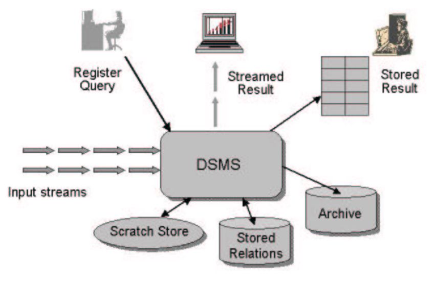
Figure 3.1.5: STREAM Query plans [14]
has developed a Data Stream Management System (DSMS) called Stanford Stream
Data Manager (also known as STREAM) [14], which integrates the SQLbased CQL
language, with the aim of processing continuous queries with many continuous data
streams. The linked paper also compares CQL with other languages.
Figure 3.1.4: Simplified Input Data Stream Management System [14]
Apache Calcite
A more recent player in the data processing world is Apache Calcite [18]. This tool
is quite multifunctional, with ability to process queries, optimize them, and support
query language. The linked work discusses the architecture behind Apache Calcite,
as well as others. It also discusses SQL extensions for geospatial queries or semi
structured data. Other mentioned extensions are data stream processing queries
extensions, or STREAM extensions. The previously stated CQL language was the
source of inspiration behind them. More information is available on their website
[65]. It is also worth mentioning that Apache Calcite is integrated by multiple DSPSs,
including Apache Flink and Apache Apex. [18]
31CHAPTER 3. RELATED WORK
Figure 3.1.6: Apache Calcite architecture and interaction [18]
Distributed Snapshot Algorithm for Flink
When it comes to Flink, the state management module includes a consistent
distributed snapshot algorithm (it resembles ChandyLamport’s protocol [26]). This
algorithm is explained in this paper [23].
Figure 3.1.7: Snapshot Algorithm [23]
32CHAPTER 3. RELATED WORK
Samza
Samza [9] was developed by LinkedIn, and its highlevel design was presented in
this paper [53]. Unlike Flink which relys on distributed snapshots, Samza replays
the change logs when attempting failure recovery. Samza uses Host Affinity to make
recoveries faster. With Samza there is no guarantee on the global consistency because
it doesn’t rely on a distributed snapshot.
Figure 3.1.8: Apache Samza [9]
Storm and Heron
In the beginning, Twitter used Storm [68] for stream data processing, but it later
switched to Heron [71]. Storm uses spouts and bolts to run apps in a distributed way.
Heron is basically the upgraded version of Storm in order to increase performance and
scalability, as well as supporting back pressure for data dropping avoidance. A self
healing and selftuning Heron version was discussed in this paper [31].
33CHAPTER 3. RELATED WORK
Figure 3.1.9: Heron [55]
Figure 3.1.10: Storm High Level Architecture [68]
3.2 Languages
SQLbased Data Stream Processing Extensions
Oracle Continuous Query Language [59] and StreamBase StreamSQL [66] are
languages intended to define streaming queries based on SQL. The difference between
these two languages was discusses in this paper [41]. The authors also attempt to unify
the two languages, but more obstacles need to be overcome.
34CHAPTER 3. RELATED WORK
Figure 3.2.1: Oracle CEP Architecture [56]
On top of Oracle CEP CQL and StreamSQL, other SQLbased data stream processing
extensions exist for specific systems, such as SamzaSQL [58] used in DSPS Samza [54],
Continuous Computation Language (CCL) used in SAP HANA Smart Data Streaming
[61], and KSQL [43] used in Apache Kafka, to name a few.
3.3 Benchmarks
Linear Road Benchmark
Generally speaking, DSPSs can be benchmarked with different tools. One of the
more popular tools is the Linear Road benchmark [16]. It is basically an application
benchmark with a toolkit for conducting benchmarks. The Linear Road benchmark in
comprised of data generator, followed by a data sender, then finally a result validator.
This benchmark was based on the concept of a variable trolling system that is used in a
metropolitan area, which has many highways with a number of cars moving. The tolls
vary depending of many aspects related to the situation of the traffic.
Reports of the different car positions are transmitted to the DSPS by the data sender.
The DSPS then either outputs data or not, depending on the traffic situation of the
highways, judged by the received reports. Other than car reports, an explicit query in
also sent as input data. An answer is always required by this explicit query. The Linear
Road benchmark paper mentions four different queries. The last one of these queries
was not implemented in the paper [16] because it was too complex.
The Lrating is basically the result of a system benchmark. The Linear Road paper
defined the Lrating as the acceptable number of highways that can tolerated by the
system all while being able to meet a certain query requirement for the response time.
The number of highways can be chosen when the data is being generated. The more
35CHAPTER 3. RELATED WORK
highways there are in the system, the higher the input rate is. In the same paper, the
Linear Road benchmark is used on a relational database as well as on a DSPS called
Aurora [1]. The paper also includes the different results.
StreamBench
StreamBench [46] is another related benchmark, with the focus on distributed DSPSs.
It can more accurately be considered as a microbenchmark because it is more suitable
to benchmark atomic operations, instead of complex applications such as it is the
case with the previously mentioned Linear Road. StreamBench includes three stateful
queries and four stateless queries, for a total of seven queries. Some of these queries
have more than one computational step, while others only have one. Unlike stateless
queries, stateful queries don’t need to keep any state to produce a correct answer or
result. When it comes to input, all queries use textual data expect one query that
processes numerical data.
Regarding the architecture of this benchmark, Apache Kafka is the message broker that
StreamBench uses for data consumption and generation, which isn’t the case with the
Linear Road benchmark. In the evaluation chapter, Apache Spark and Apache Storm
[13] are both benchmarked using StreamBench.
NEXMark
Another DSPS benchmark tool is NEXMark [51]. When it comes to Apache Beam,
NEXMark has been ported to Beam from Dataflow, and then refactored according
to the latest version of Beam. It supports all the different runners in Apache Beam.
NEXMark consists of a generator (timestamped events), NEXMarkLauncher (source
creation and launches the query pipelines), Output Metrics (such as execution time)
and Modes (batch and stream) [52].
3.4 Comparisons
Spark and Flink
A comparison of Apache Spark and Apache Flink was discussed in [49]. Multiple
queries were used in the experiments, such as grep query. The authors paid careful
attention to the changes in scaling that are affected by the total number of cluster
36CHAPTER 3. RELATED WORK
nodes. The paper doesn’t focus on the data stream perspective in the experiments
done.
Figure 3.4.1: Word count comparison between spark and flink [49]
Spark, Flink and Storm
Apache Flink, Apache Spark and Apache Storm are compared in this related paper [45].
The authors addressed the behavior in the context of a node failure. They also present
the different architectures for the DSPSs.
Figure 3.4.2: Throughput results in function of the task parallelism [45]
Spark, Flink, Apex and Beam
In the following paper [36], the authors investigate whether there are any impacts on
performance when using Apache Beam (streaming mode) with the following runners:
Spark, Flink and Apex.
37CHAPTER 3. RELATED WORK
Figure 3.4.3: Average Execution Times in s [36]
38Chapter 4
System Design and Implementation
In this chapter, we discuss how we designed the system with the intention of
conducting the different experiments.
4.1 System Design
4.1.1 Data set
The Data set that we chose is the Carbon Monoxide Daily Summary set, downloaded
from Kaggle.com. The choice of this data set was inspired by two reasons. The first one
was because it’s a relatively large enough dataset, that allows meaningful comparison
of the different data processing frameworks. The second but equal reason, was because
the nature of the data set itself is something that has meaning to us. The fact that we
can benchmark different data processing frameworks and at the same time get some
interesting insights on the Carbon Monoxide emissions is something that is likely to
be useful not only in regards to the technical aspect of engine comparison, but also for
the environmental cause.
We used the first 2 million rows of the Carbon Monoxide dataset on a hardware
consisting of 16gb of ram and an i5 8 core 8th generation CPU.
4.1.2 Queries
In order to compare the different data processing systems, in batch as well as in stream,
we will be using the 3 following queries:
39CHAPTER 4. SYSTEM DESIGN AND IMPLEMENTATION
1. Filtering: Filter the data for a specific county (filter based on a county == 31) and
get the count of records.
2. State management: Get the sum of arithmetic mean by county where state is 06
and year is 2017.
3. Windowing: Get the average of state 05 from year 1997 till 2015.
4.2 Implementation
In the following section we present the implementation of our queries in Spark, Flink,
as well as in all the runners within Beam, in batch and streaming mode.
4.2.1 Apache Beam
Apache Beam unifies both Batch and Stream processing so the code is the same for
both, which is one of the most important features offered by Beam.
Query 1
Query 1 is considered the simplest query to implement compared to the other queries.
It reads the data from the input file and parses each row individually using the map
function. It extracts the county, and creates a two valued tuple with count. After
parsing, we will have just the required information and we can filter it based on the
first tuple value which is county. So we have used the Filter operation to filter the
results for the county code 31.
Furthermore, we have grouped the different observations for each county with keyBy
operation and counted those values. Finally, the query will print a final aggregated
value for the selected county.
1 static void runQuery1 ( WordCountOptions options ) {
2 Pipeline p = Pipeline . create ( options );
3
4 // pipeline to read , filter based on county , split to kV pair , do
the count
5 p.apply(" ReadLines ", TextIO .read ().from( options . getInputFile ()))
6
40CHAPTER 4. SYSTEM DESIGN AND IMPLEMENTATION
7 .apply(new PTransform < PCollection , PCollection <
KV >>() {
8 @Override
9 public PCollection expand (
PCollection input ) {
10 return input . apply (
11 MapElements .into(
12 TypeDescriptors .kvs(
TypeDescriptors . strings () ,
TypeDescriptors . longs ()))
13 .via(line -> KV.of(line. split (",
")[1] , 1L))); //1 is
county_code since we need
filter on that;
14 }
15 })
16 .apply( Filter .by(obj -> obj. getKey (). equals ("031")))
17 .apply( Count . perKey ())
18 .apply( MapElements .via(new WordCount . FormatAsTextFn ()))
19 .apply(" WriteCounts ", TextIO . write ().to( options .
getOutput ()));
20
21 p.run (). waitUntilFinish ();
22 }
Listing 4.1: Query 1 implementation using Apache Beam
Query 2
The second query evaluates the performance of the different stream processing engine
and capabilities for stateful stream processing processing the queries which requires
state storage to complete the operation. This query implementation streams the data
from the input file, parses each row and creates a CO object with few attributes which
are going to be used for filtering. Then, the query filters the value for the state code
and for a specific year. Afterwards, each object is mapped into a key value pair of the
required information which is used to sum up all the values for a specific key, average
emission. Finally, we transform the pairs into the more user friendly strings and write
41CHAPTER 4. SYSTEM DESIGN AND IMPLEMENTATION
them into the file.
1 static void runQuery2 ( WordCountOptions options ) {
2 Pipeline p = Pipeline . create ( options );
3
4 // pipeline to read , filter based on county , split to kV pair , do
the count
5 p.apply(" ReadLines ", TextIO .read ().from( options . getInputFile ()))
6
7 .apply(new CreateCOObjects ())
8 .apply( Filter .by(obj -> obj. state_code == 6 && obj.
date_local . getYear () == 2017) )
9 .apply( MapElements
10 .into( TypeDescriptors .kvs( TypeDescriptors .
integers () , TypeDescriptors . doubles ()))
11 .via(row -> KV.of(row. county_code , row.
arithmetic_mean )))
12 .apply(Sum. doublesPerKey ())
13 .apply( MapElements
14 .into( TypeDescriptors . strings ())
15 .via(x -> x. getKey (). toString () + ": " + x.
getKey ()))
16 .apply(" WriteCounts ", TextIO . write ().to( options .
getOutput ()));
17
18 p.run (). waitUntilFinish ();
19 }
Listing 4.2: Query 2 implementation using Apache Beam
Query 3
The final query is comparing the performance of the different processing engines in
terms of windowing. It creates the grouping annually (or windows) and calculates
the mean for the windows. Similarly, it starts with streaming the data from the input
file and transforms each row into CO objects. Those objects are filtered based on the
criteria. Then, we apply the fixed size windowing on the data to see the average for
a year and calculate the mean emission. Finally, we convert objects into the pair and
42You can also read