OMEGA-open-source emission tomography software - IOPscience
←
→
Page content transcription
If your browser does not render page correctly, please read the page content below
Physics in Medicine & Biology

PAPER • OPEN ACCESS

OMEGA—open-source emission tomography software
To cite this article: V-V Wettenhovi et al 2021 Phys. Med. Biol. 66 065010

View the article online for updates and enhancements.

                               This content was downloaded from IP address 46.4.80.155 on 18/07/2021 at 17:10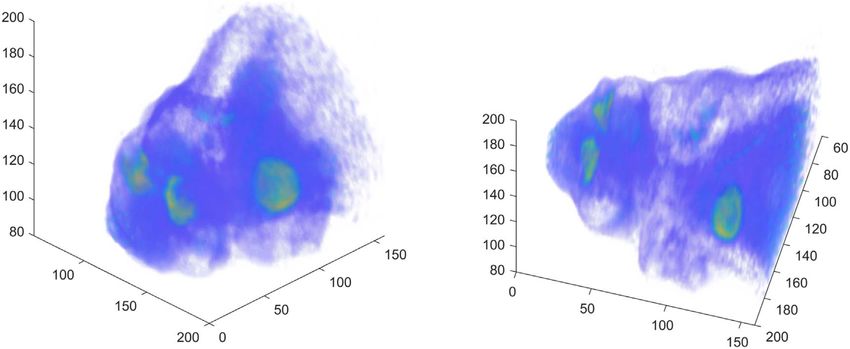
Phys. Med. Biol. 66 (2021) 065010                                                     https://doi.org/10.1088/1361-6560/abe65f

                              PAPER

                              OMEGA—open-source emission tomography software
OPEN ACCESS
                              V-V Wettenhovi          , M Vauhkonen           and V Kolehmainen
RECEIVED
30 October 2020
                              Department of Applied Physics, University of Eastern Finland, Finland

REVISED
                              E-mail: villewe@uef.fi
9 February 2021
                              Keywords: PET, positron emission tomography, image reconstruction, GPU, MATLAB, software, Octave
ACCEPTED FOR PUBLICATION
15 February 2021
PUBLISHED
4 March 2021                  Abstract
                              In this paper we present OMEGA, an open-source software, for efficient and fast image reconstruction
Original content from this
work may be used under
                              in positron emission tomography (PET). OMEGA uses the scripting language of MATLAB and GNU
the terms of the Creative     Octave allowing reconstruction of PET data with a MATLAB or GNU Octave interface. The goal of
Commons Attribution 4.0
licence.                      OMEGA is to allow easy and fast reconstruction of any PET data, and to provide a computationally
Any further distribution of   efficient, easy-access platform for development of new PET algorithms with built-in forward and
this work must maintain
attribution to the            backward projection operations available to the user as a MATLAB/Octave class. OMEGA also
author(s) and the title of    includes direct support for GATE simulated data, facilitating easy evaluation of the new algorithms
the work, journal citation
and DOI.                      using Monte Carlo simulated PET data. OMEGA supports parallel computing by utilizing OpenMP
                              for CPU implementations and OpenCL for GPU allowing any hardware to be used. OMEGA includes
                              built-in function for the computation of normalization correction and allows several other corrections
                              to be applied such as attenuation, randoms or scatter. OMEGA includes several different maximum-
                              likelihood and maximum a posteriori (MAP) algorithms with several different priors. The user can also
                              input their own priors to the built-in MAP functions. The image reconstruction in OMEGA can be
                              computed either by using an explicitly computed system matrix or with a matrix-free formalism,
                              where the latter can be accelerated with OpenCL. We provide an overview on the software and present
                              some examples utilizing the different features of the software.

                              1. Introduction

                              Positron emission tomography (PET) is a widely used medical imaging modality in both clinical and preclinical
                              settings. PET imaging can be used to investigate the distribution of biologically active radioactive tracer
                              molecules. These radioactive tracers are positron emitting molecules that are injected into the target human or
                              animal and are used to study different metabolic processes in the body. In order to obtain accurate information
                              about the metabolic processes, the measurement data needs to be reconstructed into a 3D or 4D image of
                              sufficient spatial and, in the case of 4D image, spatio-temporal resolution. Currently, iterative image
                              reconstruction methods are the gold standard in PET with numerous different algorithms already available.
                              However, there is also research effort into developing new algorithms. Therefore, it is important for researchers
                              both to be able to develop and test their new algorithms easily, but also to be able to compare them effectively
                              with current operational algorithms. Furthermore, due to the heavy computational requirements of many
                              algorithms, more efficient reconstruction implementations are needed which can be achieved with the use of
                              graphics processing units (GPUs) or multi-core CPUs.
                                   Currently there are many image reconstruction software available for PET. These include STIR (Thielemans
                              et al 2012), an open-source software capable of reconstructing PET (with or without time-of-flight, TOF) data,
                              and also includes support for single photon emission computed tomography (SPECT), including both analytic
                              and iterative reconstruction methods. PRESTO (Scheins and Herzog 2008) is a package that allows for PET
                              image reconstruction with efficient storage of the PET system matrix but has not yet been officially released.
                              TIRIUS (Leroux 2008) provides a GUI-based reconstruction of PET data but has not been recently updated.
                              EMRecon (Kösters et al 2011) allows for the reconstruction of PET data and includes for example motion
                              estimation and correction and support for TOF data. QETIR is an image reconstruction software allowing for

                              © 2021 Institute of Physics and Engineering in Medicine
Phys. Med. Biol. 66 (2021) 065010                                                              V-V Wettenhovi et al

reconstruction of both non-TOF and TOF PET data (D’Hoe 2013). J-PET Framework (Krzemien et al 2020)
is a recent software for PET data analysis and reconstruction. QSPECT (Loudos et al 2010) allows for the
reconstruction of SPECT data. For multi-modality imaging, the Michigan Image Reconstruction Toolkit
(Fessler 2019) is a MATLAB package that contains both iterative and non-iterative reconstruction algorithms for
PET, SPECT as well as for computed tomography (CT) and magnetic resonance imaging (MRI). CASToR
(Merlin et al 2018) is a fairly recent open source reconstruction package for PET (both TOF and non-TOF),
SPECT and CT. NiftyRec (Pedemonte et al 2010) supports image reconstruction in MATLAB for PET, SPECT
and CT and also includes CUDA support for Nvidia GPUs.
     In this paper we present the version 1.1 of OMEGA, open-source MATLAB/GNU Octave emission
tomography software. OMEGA is a software designed and interfaced to MATLAB (The MathWorks, Inc.,
Natick, Massachusetts, United States) and the free open-source alternative GNU Octave (Eaton et al 2020). Due
to this, either MATLAB or Octave is required in order to utilize OMEGA. The aim of OMEGA is to provide
complete software for easy and fast reconstruction of static or dynamic PET data (with or without TOF) as well as
to provide a computationally efficient,easy-access MATLAB/Octave platform for the development of new PET
imaging algorithms. OMEGA is thus designed both for those that simply want to reconstruct their data for
further analysis and for those that are interested in improving the quality of the reconstructed images by
developing their own algorithms or post-processing tools. OMEGA utilizes MATLAB/Octave-based codes as its
user-interface and for its utility functions, while also including C++ and OpenCL (Stone et al 2010) MEX codes
to enable fast image reconstruction, including efficient forward and backward projection operations using a
special MATLAB/Octave class, for any PET data. While CUDA support is available on NiftyRec, OpenCL
support is not available in any of the current PET reconstruction toolkits. OpenCL is an open standard and
supported by all the major APU, CPU and GPU manufacturers (AMD, Intel and Nvidia). Unlike previous
MATLAB-based software, OMEGA also supports data import from different formats, sinogram creation and
several corrections, including normalization correction created by OMEGA from a separate normalization
measurement. Furthermore, OMEGA includes support for a larger variety of reconstruction algorithms and
priors than previous software. OMEGA additionally includes a direct support for Monte Carlo (MC) simulated
PET data from GATE in ASCII, list-mode (LMF) or ROOT (Brun and Rademakers 1997) format. GATE is an
open-source software dedicated to numerical simulations in medical imaging (Jan 2004) and radiotherapy (Jan
et al 2011). GATE produces physically highly realistic simulation data that can be used in the design of new
medical imaging scanners, to investigate the scatter properties of an object or scanner and for evaluation of new
image reconstruction algorithms and correction techniques using simulation data from a ground truth
phantom. We remark that OMEGA could also be used to simulate (noiseless) PET measurement data by using
the forward model and then utilize the noiseless data as the expectation for the generation of (a Poisson
distributed) noisy measurement realization utilizing the MATLAB (or Octave) random number generators.
     The source code of OMEGA and all the MATLAB/Octave and GATE scripts used in section 4 are publicly
available from GitHub https://github.com/villekf/OMEGA. Documentation is included in the source package
as well as in the GitHub wiki. The Inveon list-mode PET data used in section 4 is available from https://doi.org/
10.5281/zenodo.3528056. A MATLAB add-on package containing the source files can also be downloaded from
the releases-page on GitHub. All source code is distributed under GNU General Public License v3.0.
     The paper is organized as follows. Section 2 describes the mathematical framework of PET image
reconstruction as well as the list of implemented algorithms, priors and projectors. Section 3 describes the
general software framework. In section 4 we present examples obtained with the OMEGA software. Lastly in
section 5 we discuss the further development of the software.

2. Mathematical background

This section describes the measurement data formats and algorithms that are included in OMEGA as well as the
mathematical framework in PET image reconstruction.

2.1. Measurement data formats
In PET, the measurement data is output either as a list of events, often called list-mode data, or as sinograms.
List-mode data can include the coincidences of the emitted photon pairs, delayed coincidences, gating events,
bed positions, etc. Coincidence events can, for example, contain information about the location of the detectors
that received the photons, photon energy and in recent scanners also the time-of-flight (TOF) information.
    When reconstructing images from measured PET data, the list-mode data itself can be used, where each
coincidence event is assigned to the corresponding line-of-response (LOR). These coincidences are then
processed as event-by-event basis where each coincidence is handled as a separate measurement. The LOR (or
tube-of-response, TOR, in 3D) is the line between the two detector crystals that detected the photons.

                                             2
Phys. Med. Biol. 66 (2021) 065010                                                                                 V-V Wettenhovi et al

   Figure 1. Raw data visualized with the visualizeRawData function. The data was obtained from measured Siemens Inveon PET data.
   No corrections have been applied.

     However, currently list-mode reconstruction is rarely utilized due to the large measurement data size and
more often the recorded coincidences are binned into 2D histograms, called sinograms. Sinograms are functions
of two variables, the angular variable f (tangential position) that specifies the orientation (angle) of the LOR and
the radial variable s (view) that specifies the orthogonal distance from the center of the field-of-view (FOV) to the
LOR. In a sinogram, all valid LORs are arranged according to f and s, with only LORs inside a predetermined
maximum s included. Each element of the 2D sinogram contains the total number of detected coincidences
along a LOR for a particular (f,s) combination. A separate 2D sinogram is formed for each axial ring
combination. In sinograms, the adjacent LORs are often combined in the transaxial and/or axial directions,
where the coincidences of the adjacent LORs are summed together. This summing has the effect of reducing the
number of measurement points. All the resulting sinograms are arranged together into a Michelogram.
     In OMEGA the image reconstruction can be achieved by using sinogram data, by using a list of events
containing the detector coordinates for each separate coincidence event (i.e. list-mode data) as well as by using
an alternative data format. This alternative data format is similar to sinogram data, but rather than arrange the
coincidences along the variables (f,s), the coincidences are arranged with respect to their detector indices
(numbers). This means that coincidences detected by detectors i1 and i2 are placed in element (i1, i2). This leads
to a lower diagonal matrix with a size of number of detectors × number of detectors. The lower diagonal part is
stored as a (sparse) vector. This alternative data format is called as raw data in OMEGA as it arranges the data
according to the raw detector indices without any compression or combination of adjacent LORs. Separate
function exists for the easy visualization of the raw data. Figure 1 demonstrates visually a subset of the raw data.
All features, except for TOF support, that are present for the sinogram data are also available for the raw data.
     The measurement data created by OMEGA, whether sinogram or raw data, can also be dynamic. In this case,
the data is divided into the specified number of time steps, each of equal length in time, that contain the detected
coincidences from that time interval. Each time step is stored in a different element in a cell matrix.

2.2. Image reconstruction
PET image reconstruction methods can be roughly divided into three different categories: direct methods,
analytic methods and iterative methods (Reader and Zaidi 2007).
    Direct methods, such as directly solving the least-squares estimate with e.g. the use of factorization, have not
been extensively implemented in PET image reconstruction. This is mainly due to the large size of the system
matrix A (Lewitt and Matej 2003, Reader and Zaidi 2007), which models all the image and measurement space
effects, such as the LORs. OMEGA does not include any direct methods at the moment.
    Analytic methods include the well-known filtered backprojection (FBP) in 2D and 3D reprojection in 3D
(Kinahan and Rogers 1989). Since PET data produced from modern scanners are inherently 3D, regular FBP
cannot be used without first rebinning the 3D sinogram data into 2D. Rebinning algorithms include for example

                                                      3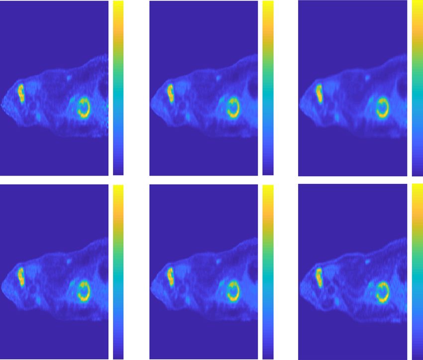
Phys. Med. Biol. 66 (2021) 065010 V-V Wettenhovi et al
single slice rebinning and Fourier rebinning (FORE) (Defrise et al 1997). Analytic methods were previously often
used in PET imaging, but currently they are no longer utilized in clinical setting. OMEGA currently does not
include analytic methods.
Iterative methods are the most widely used approach in PET image reconstruction and include iteratively
solving the maximum, either Poisson or Gaussian, likelihood (ML) or solving of the maximum a posteriori
(MAP) estimate. Poisson-based methods are a natural choice for PET since the measurements can be modeled as
Poisson processes. These can be solved by using various coordinate ascent methods, such as steepest ascent,
gradient-based methods, such as the conjugate gradient, or using functional substitution, as in maximum
likelihood expectation maximization (MLEM) (Qi and Leahy 2006, Reader and Zaidi 2007).
2.2.1. Maximum likelihood algorithms with poisson likelihood model
MLEM (Dempster et al 1977, Shepp and Vardi 1982) algorithm is a well-known method and is used to maximize
the Poisson log-likelihood. The Poisson log-likelihood is as follows
M
L ( p∣ f ) = å pi ln([ pi ]) - [ pi ] - ln( pi !) , (1)
i=1
where f is the estimated image, p the measurements, M is the number of LORs in the data and the expected value
[ pi ] = å Nj = 1 Aij f j + ri + zi . N is the number of voxels in the estimated image, ri is the estimated random
coincidences and ζi the estimated scattered coincidences.
In MLEM the image update is obtained with
f jk a ij pi
f jk + 1 = å , (2)
å i a ij i ål a il f lk + ri + zi
which is in matrix form
fk AT p
f k+1 = , (3)
A 1 Af + r + z
T k
where ∑iaij = AT1 is the sensitivity image and k the iteration number. Operation Af k corresponds to the forward
( p
)
projection while ATvk is the backprojection where v k = Af k + r + z . The inclusion of ζ and r in (2) is called the
ordinary Poisson method.
A disadvantage in using MLEM is its slow convergence. The convergence speed, however, can be accelerated
by using different methods. The most used method is the ordered subsets (OS) method, which enhances
convergence speed by dividing the measurements and the system matrix into Q subsets
f j(k, q - 1) a ij pi
f j(k, q ) = å , (4)
å a ij i Î Sq å a il f l(k, q - 1)
+ ri + zi
i Î Sq l
where Sq contains the LORs in the qth subset. Equation (4) is called the ordered subsets expectation
maximization (OSEM) algorithm (Hudson and Larkin 1994). OSEM, and other variants of the MLEM
algorithm, are widely used in the PET clinical setting. All built-in algorithms in OMEGA, except MLEM and its
MAP-variant, use subsets.
There are several different ways to select the subsets in OMEGA. These methods include for example taking
every qth measurement, taking specific angles (f) from the sinogram, using random sampling, using a sampling
method based on the golden angle (Köhler 2004) or using a constant increment scheme as in (Tanaka and
Kudo 2010).
Using OSEM, however, causes that the resulting estimate is not guaranteed to converge to the ML estimate.
Convergence, however, can be guaranteed by using a modified algorithm which uses a relaxation parameter, or
an algorithm based on the complete data of the Poisson likelihood. Relaxation methods include row-action
maximum likelihood algorithm (RAMLA) (Browne and de Pierro 1996), modified RAMLA (MRAMLA) (Ahn
and Fessler 2003), rescaled block-iterative (RBI) MLEM (Byrne 1996), dynamic RAMLA (DRAMA) (Tanaka and
Kudo 2003) and relaxed OSEM (ROSEM). Complete-data algorithms include complete-data OSEM (COSEM)
(Hsiao et al 2002) and its variants ECOSEM (Hsiao et al 2004) and ACOSEM (Hsiao and Huang 2010).
Other ML-algorithms also exists but are not included in OMEGA. These include SAGE (Fessler and
Hero 1994), OSSPS (Fessler and Erdogan 1998, Ahn and Fessler 2003) and RASAGE (Hongqing et al 2004).
Weighted least-squares (WLS) algorithms have also been utilized to solve the ML-problem (Fessler 1994), of
these the ATP-WLS (Anderson et al 1997) and SA-WLS (Zhu et al 2006) have been implemented in OMEGA as
example scripts utilizing the special forward/backward projection class.
4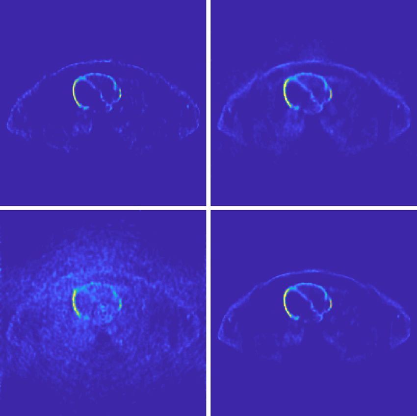
Phys. Med. Biol. 66 (2021) 065010 V-V Wettenhovi et al
Table 1. List of algorithms implemented in OMEGA.
Name Remarks References
MLEM Shepp and Vardi (1982)
OSEM Hudson and Larkin (1994)
RAMLA Browne and de Pierro (1996)
MRAMLA MBSREM-II without prior Ahn and Fessler (2003)
ROSEM Wang et al (2006)
DRAMA Tanaka and Kudo (2003)
RBI Byrne (1996)
COSEM Hsiao et al (2002)
ECOSEM Hsiao et al (2004)
ACOSEM Hsiao and Huang (2010)
MLEM-OSL MAP-algorithm Green (1990)
OSEM-OSL/OSGP MAP-algorithm Hudson and Larkin (1994)
BSREM MAP-algorithm De Pierro and Yamagishi (2001)
MBSREM MBSREM-II, MAP-algorithm Ahn and Fessler (2003)
ROSEM-MAP BSREM with ROSEM estimates
RBI-OSL MAP-algorithm Lalush and Tsui (1998)
COSEM-OSL MAP-algorithm
ACOSEM-OSL MAP-algorithm
Instead of using Poisson likelihood, it is possible to use Gaussian-based likelihoods instead. However,
Gaussian methods are not actively used in clinical setting and as such these methods are not included. These
methods can, however, be computed in OMEGA with the special forward/backward projection class. The
conjugate gradient method for least-squares (CGLS) and least-squares (LSQR) algorithms (Paige and
Saunders 1982) have been implemented as example scripts utilizing the forward/backward projection class.
2.2.2. MAP algorithms
A disadvantage of maximum likelihood estimation is its tendency to produce a noisy solution due to the noise in
the data and ill-posedness of the problem (Qi and Leahy 2006). This effect can be offset by using MAP algorithms
which complement the imaging problem with a priori information. The general MAP objective function is
defined as
F ( f ) = L ( p ∣ f ) - bR ( f ) , (5)
where R(f) is the log-prior term and β > 0 is the prior weight that determines how much emphasis is given to the
prior.
Maximizing (5) can be achieved by several different optimization methods. In emission tomography the
maximization of (5) for the Poisson log-likelihood (1) was first achieved by the one-step-late (OSL) algorithm
(Green 1990). The OSL method can be utilized to all ML-algorithms based on (1), such as MLEM, OSEM, RBI or
COSEM. Since the derivation of OSL, several other MAP-algorithms have been invented for the Poisson
likelihood, with improved convergence properties. Of these block sequential regularized EM (BSREM) (De
Pierro and Yamagishi 2001) and modified BSREM (MBSREM) (Ahn and Fessler 2003) are currently included in
OMEGA.
Alternate optimization methods maximizing (5) are implemented as example scripts of the forward/
backward projections class. These include preconditioned Krasnoselskii-Mann algorithm (PKMA) (Lin et al
2019) and alternating direction method of multipliers (ADMM) (Chun et al 2014).
Table 1 lists all the ML and MAP algorithms currently implemented (built-in) in OMEGA as well as their
references and possible remarks, such as the specific version of the algorithm and if it is a MAP algorithm. All
algorithms are also available as stand-alone MATLAB/Octave functions. Example scripts implemented with the
forward/backward projection class are included in a separate table 2.
2.3. Priors
Numerous prior functionals have been implemented in PET imaging with many based on Gibbs distribution
(Markov random fields, MRF). Table 3 lists all priors supported in OMEGA.
The general form for MRF type priors is Qi and Leahy (2006)
N
R( f ) = å å yjl ( f j - fl ) , (6)
j = 1 l Î j
5Phys. Med. Biol. 66 (2021) 065010 V-V Wettenhovi et al
Table 2. List of example algorithms included as scripts in OMEGA.
Name Remarks References
CGLS Paige and Saunders (1982)
LSQR Paige and Saunders (1982)
ATP-WLS Anderson et al (1997)
SA-WLS Zhu et al (2006)
ADMM With TV prior Chun et al (2014)
PKMA With TV or NLM prior Lin et al (2019)
Table 3. List of priors implemented in OMEGA.
Name Remarks References
1
Quadratic yjl ( f j - fl ) = 2 wQjl ( f j - fl )2 Qi and Leahy (2006)
1
Huber yjl ( f j - fl ) = 2 w Hjl w ( f j - fl )2 Fessler (1997)
MRP Based on (7) Alenius and Ruotsalainen (1997)
FMH Based on (7) Alenius and Ruotsalainen (2002)
L-filter Based on (7) Alenius and Ruotsalainen(2000),(2002),
Astola and Kuosmanen (1997)
MRP-AD Based on (7)
MRP-NLM Based on (7) Hou et al (2015)
MRP-WM Based on (7), harmonic, arithmetic and geometric mean Alenius and Ruotsalainen (2000), Astola
and Kuosmanen (1997)
WM Harmonic, arithmetic and geometric mean Hsiao et al (2001)
TV yjl ( f j - fl ) = ( f j - fl )2 , optionally can use three different anatomical Lu et al (2015), Ehrhardt et al (2016), Wet-
weighting methods tenhovi et al (2018)
∣ f j - fl ∣
SATV yjl ( f j - fl ) = ∣ f j - fl∣ - q ln 1 + ( q ) Lin et al (2019)
TGV Bredies et al (2010)
APLS With anatomic weighting only Ehrhardt et al (2016)
1
NLM yjl ( f j - fl ) = 2 w NLMjl ( f j - fl )2 Cao et al (2014)
NLTV yjl ( f j - fl ) = w NLMjl ( f j - fl )2 Zhang et al (2017)
where j is the neighborhood around voxel j and ψ is a potential function. Numerous different potential
functions have been presented (Lange 1990) such as a quadratic penalty (Hebert and Leahy 1989), the Huber
function (Huber 1981, Fessler 1997), weighted mean (WM), asymmetric parallel level sets (APLS) (Ehrhardt et al
2016), non-local means (NLM) (Buades et al 2005) and total variation (TV) (Rudin et al 1992, Jonsson et al 1998)
with both isotropic and anisotropic TV. For isotropic TV, OMEGA allows the inclusion of anatomical
information into the prior with three different methods, presented in (Lu et al 2015, Ehrhardt et al 2016,
Wettenhovi et al 2018). Table 3 also shows the potential functions currently implemented in OMEGA.
Some priors cannot be expressed with (6). Such priors included in OMEGA are the median root prior (MRP)
(Alenius and Ruotsalainen 1997) and total generalized variation (Bredies et al 2010, Knoll et al 2015).
MRP is defined as
1 ( f - Med ( f ))2
R( f ) = , (7)
2 Med ( f )
where Med(f) is the (constant) median filtered image (estimate). The median image in (7) can be replaced with
differently filtered image. Such modifications included in OMEGA are the finite impulse response median
hybrid (FMH) (Alenius and Ruotsalainen 2002), L-filter (Alenius and Ruotsalainen 2000, 2002, Astola and
Kuosmanen 1997), MRP-WM (arithmetic, geometric or harmonic mean) (Astola and Kuosmanen 1997, Alenius
and Ruotsalainen 2000), anisotropic diffusion (MRP-AD) and MRP-NLM.
TGV (Bredies et al 2010) differs from TV in that it does not assume the image to be piecewise constant. TGV
has been used previously in PET in joint PET-MRI reconstruction (Knoll et al 2015). In OMEGA, however, TGV
is implemented as a regular prior utilizing only the PET information.
The priors included in table 3 can be run as stand-alone MATLAB/Octave functions and output the gradient
of the prior. Some priors, mentioned in the function documentation, also allow to output the MRF-function (6).
The PKMA and ADMM examples mentioned in section 2.2.2 also serve as examples demonstrating the use of
priors in custom code with the included TV and NLM priors.
6Phys. Med. Biol. 66 (2021) 065010 V-V Wettenhovi et al
It is also possible for the user to use custom gradient-based priors in OMEGA. This is achieved by inputting
the gradient of their own prior to any of the MAP-algorithms listed on table 1. The gradient of the custom prior
has to be computed manually in MATLAB/Octave but can then be automatically included to the selected
algorithm(s).
2.4. System matrix formation
The system matrix A, and the forward and backward projections it is used in, constitute computationally the
most significant portion of the PET image reconstruction. In OMEGA, however, it is also possible to compute
the forward (Af) and backward (ATy projections, where y is any vector with the same dimensions as the
measurement vector p) matrix-free, i.e. without explicitly assembling the system matrix A. The system matrix
can be used to model various effects in the detector and image space. The system matrix A can be decomposed
into several components each modelling a different effect
A = gC LOBGH, (8)
where γ is a positive global correction factor that is identical for all LORs, C is a diagonal matrix containing the
normalization coefficients for each LOR, Λ models the effects of scatter, O is the projection blurring matrix
(includes e.g. depth of interaction effects), B is a diagonal matrix containing the probability of attenuation along
each LOR, G is the geometric projection matrix, and H is the image blurring matrix (includes e.g. positron range)
(Iriarte et al 2016). OMEGA, however, only outputs the system matrix A, e.g. none of the submatrices are
explicitly formed. If no corrections are applied, or the corrections are applied directly to the measurement data,
the matrix G equals the system matrix.
2.4.1. Geometric projection matrix
The geometric projection matrix, G, models the geometric effects. A single element, gij, of the matrix G describes
the probability that an event originating from voxel j is detected in LOR i. The elements of the matrix can be
determined by three different methods: empirical methods, MC methods, and analytical methods (Iriarte et al
2016).
Due to the time constraints of the empirical and computational constraints of the MC methods, analytical
methods are most often used and thus implemented in OMEGA. Analytical projection methods are fast and can
be computed on-the-fly during reconstruction. The basic principle is commonly either a ray-tracing or a
distance-based approach. In OMEGA, three different analytical methods are implemented: an improved version
(Jacobs et al 1998) of the Siddon’s algorithm (SRT) (Siddon 1985), the orthogonal distance-based ray tracer
(ODRT) (Aguiar et al 2010) and the volume-based ray tracer (VRT) originally included in the THOR (Lougovski
et al 2014) algorithm.
In SRT we follow the ray in the voxel grid and determine the voxel indices of intersection between the ray and
the grid. For each voxel, the length of the line of intersection is determined and then normalized with the length
of the ray to obtain the probability of emission. Each ray, or in this case LOR, is processed separately.
SRT can be extended to multiple rays to improve the accuracy of the projector (Markiewicz et al 2005). While
different methods exist for computing multiple rays (Markiewicz et al 2005, Cecchetti et al 2013, Cloquet et al
2010), in OMEGA the multi-ray Siddon is achieved by replacing the single LOR located in the center of both the
detectors with a total of Mrays equally spaced LORs and then averaging the probabilities. The user can specify the
number of rays separately for the transaxial and axial directions with the total number of rays being the
multiplication of these two values.
Orthogonal distance-based ray-tracer combines both a ray-tracer and a distance-based approach. First, we
follow the ray just as in SRT, but at each intersection (voxel) we compute the element gij as
d ij
gij = 1 - , (9)
FWHM
where dij is the orthogonal distance between the center of the voxel of interest and the LOR, and FWHM the full
width at half maximum for the PET system. To accelerate computations, values of gij below 0.01 are ignored in
OMEGA.
Volume-based ray-tracer again uses the SRT to follow the ray. In VRT, however, we make two
approximations in order to obtain a computationally feasible ray-tracer. We first approximate the voxels as
spheres and the tube between the detectors is approximated as a cylinder. These approximations enable for the
analytical computation of the volume of intersection between the sphere and the cylinder (Lamarche and
Leroy 1990). The orthogonal distance between the center of the cylinder and the center of the sphere is used to
obtain the volume of intersection value. The probability of emission for each voxel is then computed by dividing
each volume of intersection with the total volume of the LOR.
TOF In TOF, the time difference between the two detected photons is stored with a certain level of accuracy
that is dependent on the crystals used. The accuracy of the geometrical projection matrix is then enhanced as the
7Phys. Med. Biol. 66 (2021) 065010 V-V Wettenhovi et al
most probable location of the gamma photons can be narrowed according to the accuracy of the time difference
measurement. All recent clinical PET/CT scanners have TOF ability and most PET/MRI scanners as well
(Vandenberghe et al 2016) with the best clinical TOF time resolution being approximately 214 ps (van Sluis et al
2019).
The TOF implementation in OMEGA is similar to the ones described in (Lois et al 2010, Filipović et al 2019).
The TOF weights are obtained by integrating a 1D Gaussian probability density function along the LOR, where
the mean value is obtained from the center of each TOF time bin and the variance from the full width at half
maximum of the time difference accuracy. The integration itself is computed with trapezoidal rule. These TOF
weights are then normalized such that for each voxel j on every LOR i the sum of all TOF time weights is one. Due
to the TOF operating on LORs, ODRT and VRT are not supported.
2.4.2. Attenuation
The diagonal matrix B corrects for the loss of counts due to attenuation. Each diagonal element of B describes
the probability that a photon was attenuated along the specific LOR. Matrix B is computed with
⎛ Ni ⎞
bii = exp ⎜⎜ - å gˆij mj ⎟⎟ , (10)
⎝ j ⎠
where gˆij is the length of line of intersection of voxel j in LOR i, μj the attenuation coefficient for voxel j and Ni the
amount of voxels along the LOR. When using multi-ray LOR, the attenuation is computed as the average of
all rays.
Attenuation correction can be applied by using either CT or MRI images, or computing the ratio of counts
between a blank and transmission scans. When using CT or MRI data, the attenuation values need to be scaled
for 511 keV photons by using, for example in the case of CT, trilinear interpolation (Abella et al 2012). When
using separate blank and transmission scans, the ratio of counts obtained by dividing the transmission scan with
the blank scan is reconstructed into an attenuation image. As the blank and transmission measurements are
obtained by using isotopes with different energy than the usual 511 keV, the obtained image needs to be scaled
for the 511 keV attenuation coefficients by interpolating the coefficients values. If attenuation correction is
performed in the sinogram domain rather than in the reconstruction phase, the attenuation image is forward
projected (Aμ) into a sinogram and multiplied with the measurement sinogram.
When using CT data, OMEGA includes a function to automatically convert the CT-attenuation images into
511 keV attenuation images. In MRI, the user needs to manually convert them into either CT equivalent images
or into 511 keV attenuation images. With blank and transmission scans, the user needs to divide them to obtain
the relative counts and then reconstruct attenuation images or manually multiply the relative counts with the
measurement data (in which case B = I). In OMEGA, automatic attenuation is included only in the
reconstruction phase using user-input attenuation images.
2.4.3. Image blurring matrix
Modelling image resolution effects consists, for example, correcting for the detector resolution and positron
range (Iriarte et al 2016). Each element hjj ¢ of the image blurring matrix H represents the probability that a
detected event from voxel j actually originated from voxel j′. While there are many ways to implement the image
blurring matrix, the simplest approach is to use a shift-invariant Gaussian point spread function (PSF) (Iriarte
et al 2016).
In OMEGA, the image blurring is implemented by using 3D convolution with a 3D Gaussian function in the
forward projection, backward projection and in the sensitivity image. The method used in OMEGA is similar to
the one described in Antich et al (2005). The user needs to input the FWHM of the Gaussian for all three
dimensions.
2.4.4. Projection blurring matrix
Projection space effects include depth of interaction (parallax error) and inter-crystal scattering (Iriarte et al
2016), i.e. blurring that occurs in the detection space. Positron range effects can also be included (Alessio et al
2010). Each element of O represents the probability that an event detected along LOR i actually originated along
LOR i ¢. The projection space effects can be included by using e.g. spread functions. Projection effects are not
currently modeled in OMEGA.
2.4.5. Normalization
The system normalization matrix, Q, describes the differences in the sensitivity along each LOR. These
differences can be due to different detector efficiencies, detector geometry or photomultiplier tube gain. Since
8Phys. Med. Biol. 66 (2021) 065010 V-V Wettenhovi et al
Figure 2. A schematic image of the three different layers in OMEGA and their core functions.
normalization contains many different effects, the matrix Q can be split into different components, each
modelling different aspects of the scanner. This is called component-based normalization.
The component-based normalization implemented in OMEGA is based on the components presented in
Meikle and Badawi (2005). These components are: axial block profile factors, axial geometric factors, detector
efficiencies, transaxial block profiles, and transaxial geometric factors. Alternatively, the user can also input their
own normalization file.
2.4.6. Scatter
Scatter matrix, Λ, describes the probability for scatter along the specific LOR. Conventionally the scatter matrix
is a full matrix where each element l jj ¢ describes the probability that an event originating from LOR j′ detected in
LOR j has not scattered. In OMEGA, however, the scatter correction matrix can only be included as a vector
containing the diagonal elements, leading to a diagonal matrix Λ that simply describes the probability of scatter
in each LOR.
In the ML-framework, scatter can be alternatively included additively in the forward projection (as in (2)). In
this case Λ = I.
2.4.7. Global correction factor
The global correction factor γ can be used to correct all LORs with the same coefficient. This can be e.g. decay
correction or dead time correction. In OMEGA, the global correction factor is an optional scalar value that the
user can set.
3. Software framework
3.1. Overview
OMEGA consists of three different embedded layers, each utilizing a different computing language and where
each subsequent layer depends on the previous layer(s). The first, and top, layer is the only one that is directly
exposed to the user and which can also be modified by the user without the need for any recompilation of the
code. This top layer consists of the MATLAB/Octave scripts and functions that, when necessary, call the middle
C++ MEX-layer. The middle layer can perform the image reconstruction step itself, transfer the necessary
variables and call the bottom, OpenCL, layer or be used to load specific input measurement data (ROOT, LMF
and list-mode). Figure 2 shows a schematic of the general workflow of each layer.
The top layer contains most of the included functions in OMEGA and as such allows the easy modification of
these functions as well as the possibility to add additional functions, such as different correction algorithms, with
relative ease. All the operations, including system matrix formation, except for loading of ROOT, LMF or list-
9Phys. Med. Biol. 66 (2021) 065010 V-V Wettenhovi et al
mode binary data are possible to perform on the first layer. For system matrix formation, however, this is only
considered as a fallback or testing method. The other layers perform only specialized tasks in order to achieve
higher computational speed than would be achievable in a pure MATLAB/Octave function. These include
sinogram creation, load of specific data formats, system matrix creation and computing the image
reconstruction matrix-free including the forward and backward projection operators.
The user primarily controls the top layer with the use of a settings files, named as main-files, although
practically all included functions can be called stand-alone. In a such main-file, the user defines input variables,
such as the scanner specific properties, and then selects what options, such as what corrections are applied and
what reconstruction algorithm is used, with a true/false selection.
Several different main files are included. These include main-file for general PET-data, GATE MC-simulated
PET data, PET data utilizing a custom user-made gradient-based prior, a simplified main-file for GATE-
simulated data that contains only very limited number of adjustable settings and a main-file containing example
scripts on solely computing the forward (Af) and/or backward (ATy) projections (algorithms previously
mentioned in sections 2.2.1 and 2.2.2). These forward and backward projection operations provide the user an
easy access to high performance system matrix operations that are needed in implementations of new image
reconstruction algorithms. Furthermore, main-files are included for three different scanners such that all the
scanner specific parameters have been automatically set. These scanners are Siemens Inveon PET, Siemens
Biograph mCT and Siemens Biograph Vision. In all three cases, the scanner list-mode data can be used or,
alternatively, GATE simulated data. Each main-file stores the input parameters in a structure variable that is used
as an input to the core top layer functions.
The main file for general PET-data can be used with any PET scanner and data as long as it is either in
sinogram format or in the same raw data format as used by OMEGA (see section 2.1). The input measurement
data can be a mat-file, Interfile, NIfTI file, Analyze 7.5 file, DICOM file, MetaImage file or a file in binary format.
Main file for GATE-data includes GATE-specific settings and automatically loads the selected GATE output
data (LMF, ASCII or ROOT) or previously created GATE measurement data, depending on user selections. The
scanner specific main-files mentioned in an earlier paragraph function exactly as the GATE-specific main-file
except for also allowing the load the scanner specific list-mode data or scanner created sinogram data.
A modified version of the general PET-data main-file allows the use of user-made custom gradient-based
prior in any of the built-in MAP algorithms (see table 1). This gradient is automatically included to the selected
algorithm(s). While this is built on the general PET-data main-file, the functions used within can take input from
any main-file.
Lastly, a main-file exists that provides examples on how to compute the forward (Af) and/or backward
projections (ATy) with any input vector. This elaborates on how to implement the forward and/or backward
projection operations needed, for example, when developing new custom algorithms (mentioned as examples in
section 2.2). These can be either computed using specific functions or by taking advantage of a special
MATLAB/Octave class. The class object, after it has been constructed, can then be simply multiplied with the
desired vector in MATLAB/Octave. Both operations can be computed completely matrix-free on the chosen
OpenCL device or simply on the CPU through C++. The sensitivity image can also be obtained from the same
class. This class can also output the system matrix, or a subset of it, instead of using the matrix-free methods.
The general layout of all main-files, with the exception of the forward/backward projections example, is
largely the same. The first section of the file contains the adjustable input parameters. Next is an optional
precomputation phase that computes the number of voxels that each LOR will pass through. This is used to skip
any LORs that do not intersect with the FOV and in the matrix version to preallocate the correct amount of
memory for the system matrix. GATE and scanner specific files then contain functions to load the measurement
data and in certain scanners to load the attenuation data. Next are optional functions to perform selected
corrections to the sinogram or compute the normalization coefficients from the input measurement data. In the
last part is the function to perform image reconstruction.
Below we present the property variables related to the core functionality of the software.
3.2. Scanner requirements
In OMEGA this subsection is used to input the necessary parameters related to scanner geometry and is
compulsory in all cases. The required information are the number of blocks in both transaxial and axial
directions, number of crystals per block in transaxial and axial directions, crystal pitches/sizes, FOV and bore
diameter. Each block (also called buckets and in GATE as rsectors/modules/submodules) contains X × Y
number of crystals. The total number of blocks in axial direction times the Y number of crystals per block in axial
direction should equal the number of crystals in the axial direction. Crystal pitch is the distance between the
centers of adjacent crystals and has to be specified separately for the transaxial and axial directions. For FOV,
there are separate parameters for the X-, Y- and Z-directions, where X and Y are the transaxial dimensions. In
10Phys. Med. Biol. 66 (2021) 065010 V-V Wettenhovi et al
OMEGA, the Y-direction is the horizontal (column) direction and X-direction the vertical (row) direction. Z-
direction is the axial dimension. The diameter of the bore is the distance between two opposite detectors.
Furthermore, some scanners, like Siemens Biograph mCT, use additional pseudo detectors and rings in
addition to the physical detectors and rings, to achieve equidistant spacing between detectors and rings. While
these pseudo detectors do not physically exist, they can be taken into account in OMEGA. Separate variables
exist for the number of pseudo rings (the pseudo rings are assumed to be distributed between equal number of
physical rings) and the number of detectors on a single crystal ring including the pseudo detectors. Pseudo
detectors should only be used when the real scanner in question uses them and you wish to use similarly
formatted measurement data. Pseudo detectors and rings are ignored if using raw data.
3.3. GATE specific features
This subsection describes the special features available only for GATE data. First, ASCII, LMF and ROOT
formatted GATE output data can be automatically imported into MATLAB/Octave with OMEGA. In addition
to saving prompt coincidences, the user can choose to save also trues, randoms, scatter and delayed
coincidences. Prompts include all the measured coincidences except the delayed coincidences and can be
described as
pprompts, i = ptrues, i + pscatter, i + prandoms, i , (11)
where pprompts,i are prompt coincidences of LOR i, ptrues,i the true coincidences, pscatter,i the scattered
coincidences and prandoms,i the random coincidences. Trues include only coincidences that have not scattered
and originate from the same annihilation event. Randoms include the actual random coincidences included in
prompts and originate from different annihilation events. Randoms differ from delayed coincidences and
provide the exact randoms distribution of the measurement. Scatter includes all coincidences that originate
from the same annihilation event but have undergone Compton and/or Rayleigh scattering at least once.
Delayed coincidences are obtained from a delayed coincidence window and can be used in randoms correction
(see section 3.4).
For scatter data, it is also possible to differentiate the different types of scattered events as well as the number
of times the photon has scattered. GATE stores different scatter values for the Compton scattering in the
phantom and in the detector as well as Rayleigh scattering in the phantom and in the detector. The user can
choose to include any, or all, of these scatter components in the scatter data and to include, for example, only
Compton scattered events in the phantom that have scattered twice or more.
Furthermore, a true decay image can be obtained. This image contains the actual number of coincidences
that have emitted from a certain voxel. In OMEGA this image can be formed in several different ways, such as
obtaining the coordinates of the true annihilation events and placing the events in the corresponding voxel.
Similar images can be obtained for scatter and randoms but using a single photon (singles) mode.
GATE data can be converted to TOF data from non-TOF data in OMEGA. The user can specify the desired
time resolution, number of TOF bins and the length for all the bins. This process is automatically performed
during the data import.
3.4. Corrections
Several corrections can be applied either directly to (precorrect) the measurement data (sinogram or raw data) or
included in the system matrix (forward and backward projections and sensitivity image). Currently randoms,
attenuation, normalization, arc and scatter correction can be included in OMEGA. Sinogram/raw data vector
can be precorrected with normalization, randoms, scatter and arc correction. Alternatively, normalization,
attenuation, randoms and scatter can be corrected during the reconstruction as in the ordinary Poisson (3).
Randoms correction data can be obtained automatically from delayed coincidences when using GATE data
or Inveon/mCT/Vision list-mode data. Alternatively, the user can input their own randoms correction data as a
mat-file. The input randoms correction data can be either subtracted from the sinogram/raw data
(precorrection) or included in the reconstruction as r in (2).
The randoms data can be optionally smoothed and/or go through a variance reduction. The randoms
variance reduction has been implemented with 3D fan-sum algorithm and smoothing with a fixed 7 × 7 moving
mean window (Badawi et al 1998, 1999). As both are implemented as independent MATLAB functions, the user
can easily modify either of the functions with their own implementations without changing any other aspects of
the software.
Scatter correction in OMEGA can be implemented by inputting a user-specified scatter correction data
(sinogram or raw data format). As with randoms correction, it can be either subtracted from the sinogram/raw
data or included in the reconstruction as ζ in (2). In addition to these scatter data can be alternatively included in
the system matrix as the diagonal probability matrix Λ. While scatter correction itself cannot be computed in
OMEGA, a scatter measurement data from GATE simulations can be extracted and used as the scatter correction
11Phys. Med. Biol. 66 (2021) 065010 V-V Wettenhovi et al
data ζ. The scatter data can be optionally smoothed with the same moving mean smoothing and processed with
the variance reduction as with randoms data. Scatter data can also be separately normalized when normalization
is applied.
Attenuation correction is implemented in the system matrix A and is thus only possible during the image
reconstruction phase. The attenuation data (e.g. CT-images scaled to 511 keV) has to be provided by the user.
Additional functions exist that automatically scale the attenuation data from CT-images (trilinear interpolation
(Abella et al 2012)) or from 122 keV (Germanium-68 source) into 511 keV attenuation coefficients.
Attenuation correction is computed identically for SRT, ODRT and VRT. Although ODRT and VRT
comprise of more voxels and spread to the neighboring voxels along the ray, the attenuation is still assumed to
occur along the same ray as in SRT in order to simplify the computations. Normalization correction can be
either calculated directly in OMEGA with normalization measurement data or included as a user specified
MATLAB mat-file/Inveon nrm-file. The sinogram/raw data can be either precorrected for normalization
or applied during the reconstruction phase in the system matrix A. When using precorrected data the
normalization data is multiplied with the measurement data. For computing the normalization coefficient, it is
recommended to use measurement data that has uniformly distributed radioactivity distribution, for example
by using a rotating source, in order to avoid errors and artefacts in the normalized data. OMEGA supports
normalization correction for both sinogram data as well as for the raw data format. 3D fan-sum algorithm is
available for sinogram data while both the 3D fan-sum and 3D Casey (Casey and Hoffman 1986, Badawi et al
1998) are available for raw data. The computing of the normalization coefficients is handled in a MATLAB/
Octave function and can thus be easily modified to support other algorithms. For raw data, the normalization
coefficients are computed differently from sinogram data and as such the used algorithms for raw data are not
exactly the same as in the literature.
In arc correction the orthogonal distances between adjacent LORs with the same angle are made equidistant,
as the circular configuration of most PET designs causes the adjacent LORs not to be equidistant. Using the
original detector coordinates and the new detector coordinates of equidistant LORs, the sinogram is
interpolated into this new detector grid. This procedure would be mandatory when using analytical methods
such as FBP but is not required with iterative methods. However, since the measurement data becomes equally
spaced it will remove aliasing artifacts in certain cases (e.g. with Inveon data). As with randoms and
normalization, the arc correction is a separate MATLAB/Octave function.
3.5. Image reconstruction
Image reconstruction in OMEGA can be performed either for static data or for dynamic data that contains any
number of time steps. For dynamic data, the measurement data is divided into user specified number of time
windows and each time window is reconstructed independently. Image reconstruction is available for sinogram
data, raw data as well as pure event-by-event (list-mode) data. In all cases, the values of the reconstructed 3D
images show the number of counts per image voxel. This can be scaled to Bq/mL with the scaleImages function
in OMEGA. First the user needs to choose one of the four ways to implement the image reconstruction, referred
to as implementations. Each implementation additionally has two different modes of working, one with a
precomputation phase and one without. The advantage of using precomputation is that all LORs that do not
intersect the FOV are automatically ignored and as such there is no validation whether the LOR in question
intersects with the FOV which in turn speeds up the computations. All the three geometric projectors mentioned
in section 2.4.1 can be used with any implementation and any algorithm. Table 4 shows which algorithms are
supported by each implementation.
Table 4 summarizes the algorithms that are supported by each implementation as well as the key features and
requirements of each implementation. All four implementations are briefly summarized here.
3.5.1. Implementation 1
• System matrix A computed in a MEX-file and can be imported to MATLAB/Octave (OpenMP C++ (Dagum
and Menon 1998))
• Uses the full (or a subset of) system matrix A
• Allows calling of forward (Af) and backward (ATy) projection class (matrix form)
• Contains a fallback pure MATLAB/Octave code
• Image reconstruction phase itself performed in MATLAB/Octave
• Any number of and any algorithms and priors can be selected
12Phys. Med. Biol. 66 (2021) 065010 V-V Wettenhovi et al
Table 4. Algorithms and features supported/required by each implementation.
Algorithm Implementation 1 Implementation 2 Implementation 3 Implementation 4
MLEM X X X X
OSEM X X X X
RAMLA X X X
MRAMLA X X
ROSEM X X X
DRAMA X X X
RBI X X X
COSEM X X X
ECOSEM X X X
ACOSEM X X X
MLEM-OSL X X X
OSEM-OSL X X X
BSREM X X X
MBSREM X X
ROSEM-MAP X X X
RBI-OSL X X X
COSEM-OSL X X X
ACOSEM-OSL X X X
Feature
Extract A X
Af, ATy class X X X
Matrix-free X X X
OpenMP X X
OpenCL X X
CUDA X
ArrayFire X
Multi-device OpenCL X
Double precision X X
Single precision X X
TOF X X X
List-mode reconstruction X X X
• Slowest
• Requires only C++11 compiler
3.5.2. Implementation 2
• Matrix-free OpenCL or CUDA
• Requires the open-source ArrayFire library (Yalamanchili et al 2015)
• The recommended and fastest implementation with one device
• Any number of and any algorithms and priors can be selected
• Supports event-by-event (list-mode) reconstruction
• Implementation 2 uses single precision and is not numerically as accurate as implementations 1 and 4
3.5.3. Implementation 3
• Matrix-free OpenCL
• Allows calling of forward (Af) and backward (ATy) projection class (matrix-free)
• Allows the use of multiple devices, even CPU+GPU (only from same manufacturer)
• Only OSEM or MLEM can be computed
• Recommended for custom forward and backward projection code and multi-device cases
13Phys. Med. Biol. 66 (2021) 065010 V-V Wettenhovi et al
• Supports event-by-event (list-mode) reconstruction
• Implementation 3 uses single precision and is not numerically as accurate as implementations 1 and 4
3.5.4. Implementation 4
• Matrix-free OpenMP C++
• Default implementation
• Allows calling of forward (Af) and backward (ATy) projection class (matrix-free)
• Supports event-by-event (list-mode) reconstruction
• Faster than implementation 1, but slower than 2 or 3
• Requires only C++11 compiler
3.6. Data import and export
Other types of input data can be used in OMEGA, in addition to the three supported GATE output formats and
Inveon/Biograph data. When using PET data, the user can input measurement data (e.g. sinograms) as a
MATLAB/Octave mat-file, DICOM images, Interfile binary data, Analyze 7.5 data, NIfTI data, MetaImage file
or a raw binary data.
For data export the same options are available as with import. Automatic MATLAB/Octave functions exist
for both sinogram data and reconstructed images. The exported data could then be used in other software such
as for example ITK (Yoo et al 2002) for image registration, PETPVC (Thomas et al 2016) for partial volume
correction or Carimas (Nesterov et al 2009) for time-activity curves. OMEGA does not include functions to for
clinical analysis, such as computing the standard uptake values, and as such these need to be computed either
with 3rd party software or by user-made function. Alternatively, one could also export the GATE/Inveon/
Biograph data sinogram and use it in some other reconstruction software or in their own code.
3.7. Visualization
OMEGA includes several visualization codes for the reconstructed images. In all static cases the visualization
goes through all the slices in the image separately, with the selected view (transverse, frontal or sagittal).
Automatic visualization is available to every algorithm at their last iteration, optionally side-by-side with the
original GATE decay image when using GATE simulated data. Additionally, visualization is available to one
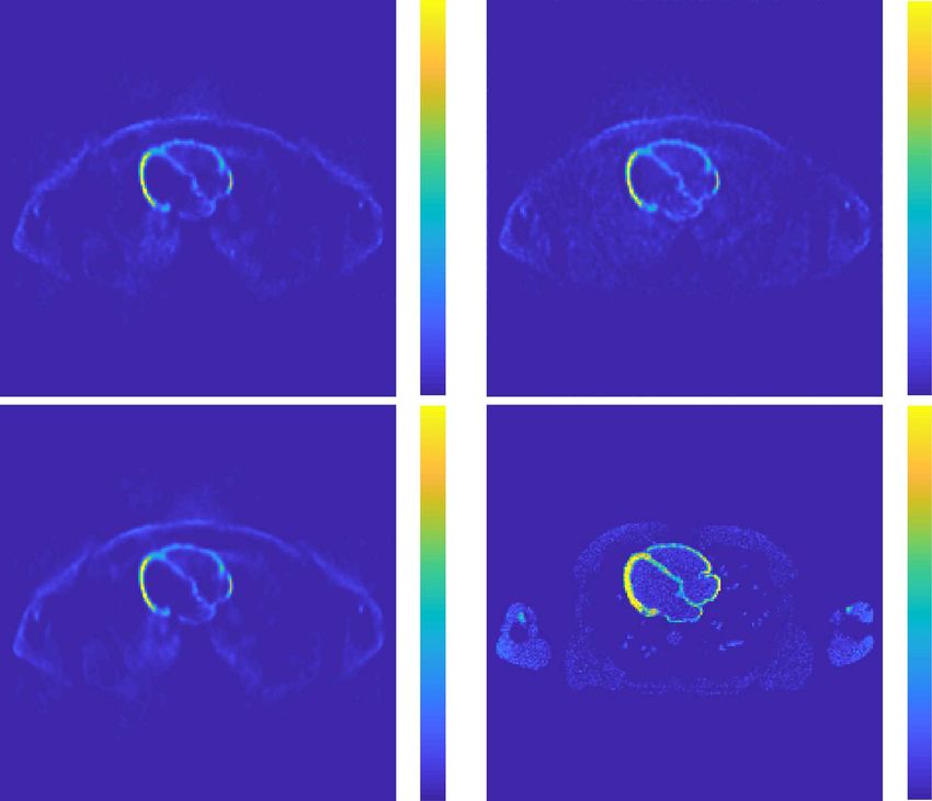
algorithm with selected number of iterations, visualizing all slices as a 3D volume with vol3D v2
(Woodford 2011) and simultaneous visualization of all the views for one algorithm. Dynamic visualization is
available for time-varying cases where a selected slice and view from selected algorithms is visualized as a
function of time.
4. Examples
Here we present some examples of the OMEGA software with both simulated and measured preclinical PET
data. In both cases, the shown results are obtained by using implementation 2 and are reconstructed in 3D.
Implementation 2 was chosen since it both supports all the algorithms as well as is faster and more memory
efficient than implementations 1 and 4. Only a small subset of the algorithm and prior combinations are
presented here due to the sheer number of possible combinations. A thorough comparison and examination
of the different methods is out of the scope of this paper.
4.1. Simulated data
Simulated PET data was obtained from GATE by using the XCAT (Segars et al 2010) human phantom. The
scanner used in the simulations was a 4-ring Siemens Biograph mCT PET/CT. The simulated radionuclide was
O-15 as gamma photons and exhibited the highest concentration in the cardiac muscles. The simulations were
not based on any actual clinical measurement and were obtained such that the total number of counts, as well as
scatter properties, were sufficiently large to visually discern the heart. Two different simulation data sets were
summed together to improve the statistics. Static phantom was used and, as a result, the simulation data
can be considered to be a single gate in a gated cardiac examination. All reconstructed images are of size
200 × 200 × 109 and were reconstructed with the OSEM algorithm with a total of 10 iterations and 8 subsets.
Improved Siddon was used as the projector with PSF enabled. FWHM of the PSF was set as 1.5× crystal pitch in
14You can also read