REGULARIZED OPTIMAL TRANSPORT FOR DYNAMIC SEMI-SUPERVISED LEARNING
←
→
Page content transcription
If your browser does not render page correctly, please read the page content below
R EGULARIZED O PTIMAL T RANSPORT FOR DYNAMIC
                                                                  S EMI - SUPERVISED L EARNING

                                                                                       Mourad El Hamri, Younès Bennani
                                                                             Université Sorbonne Paris Nord, LIPN 7030 UMR CNRS
arXiv:2103.11937v2 [stat.ML] 25 Mar 2021

                                                                                 LaMSN - La Maison des Sciences Numériques
                                                                                  name.surname@sorbonne-paris-nord.fr

                                                                                                    A BSTRACT
                                                       Semi-supervised learning provides an effective paradigm for leveraging unlabeled data to improve
                                                       a model’s performance. Among the many strategies proposed, graph-based methods have shown
                                                       excellent properties, in particular since they allow to solve directly the transductive tasks according to
                                                       Vapnik’s principle and they can be extended efficiently for inductive tasks. In this paper, we propose
                                                       a novel approach for the transductive semi-supervised learning, using a complete bipartite edge-
                                                       weighted graph. The proposed approach uses the regularized optimal transport between empirical
                                                       measures defined on labelled and unlabelled data points in order to obtain an affinity matrix from
                                                       the optimal transport plan. This matrix is further used to propagate labels through the vertices of the
                                                       graph in an incremental process ensuring the certainty of the predictions by incorporating a certainty
                                                       score based on Shannon’s entropy. We also analyze the convergence of our approach and we derive
                                                       an efficient way to extend it for out-of-sample data. Experimental analysis was used to compare the
                                                       proposed approach with other label propagation algorithms on 12 benchmark datasets, for which we
                                                       surpass state-of-the-art results. We release our code. 1

                                           Keywords Semi-supervised learning · Label propagation · Optimal transport

                                           1       Introduction
                                           Semi-supervised learning has recently emerged as one of the most promising paradigms to mitigate the reliance of
                                           deep learning on huge amounts of labeled data, especially in learning tasks where it is costly to collect annotated data.
                                           This is best illustrated in medicine, where measurement require overpriced machinery and labels are the result of an
                                           expensive human assisted time-consuming analysis.

                                           Semi-supervised learning (SSL) aims to largely reduce the need for massive labeled datasets by allowing a
                                           model to leverage both labeled and unlabeled data. Among the many semi-supervised learning approaches, graph-based
                                           semi-supervised learning techniques are increasingly being studied due to their performance and to more and more
                                           real graph datasets. The problem is to predict all the unlabelled vertices in the graph based on only a small subset
                                           of vertices being observed. To date, a number of graph-based algorithms, in particular label propagation methods
                                           have been successfully applied to different fields, such as social network analysis [7][50][51][25], natural language
                                           processing [1][43][3], and image segmentation [47][10].

                                           The performance of label propagation algorithms is often affected by the graph-construction method and the
                                           technique of inferring pseudo-labels. However, in the graph-construction, traditional label propagation approaches
                                           are incapable of exploiting the underlying geometry of the whole input space, and the entire relations between
                                                   Paper submitted to Pattern Recognition
                                               1
                                                   Code is available at https://github.com/MouradElHamri/OTP
labelled and unlabelled data in a global vision. Indeed, authors in [53][52] have adopted pairwise relationships
between instances by relying on a Gaussian function with a free parameter σ, whose optimal value can be hard to
determine in certain scenarios, and even a small perturbation in its value can affect significantly the classification
results. Authors in [48] have suggested to derive another way to avoid the use of σ, by relying on the local concept of
linear neighborhood, though, the linearity hypothesis is intended just for computational convenience, a variance in
the size of the neighborhood can also change drastically the classification results. Moreover, these algorithms have
the inconvenience of inferring pseudo-labels by hard assignment, ignoring the different degree of certainty of each
prediction. The performance of these label propagation algorithms can also be judged by its generalization ability for
out-of-sample data. An efficient label propagation algorithm capable of addressing all these points has not yet been
reported.

One of the paradigms used to capture the underlying geometry of the data is grounded on the theory of opti-
mal transport [46][38]. Optimal transport provides a means of lifting distances between data in the input space to
distances between probability distributions over this space. The latter are called the Wasserstein distances, and they
have many favorable theoretical properties, that have attracted a lot of attention for machine learning tasks such as
domain adaptation [15][16][14][6][36], clustering [28][12][9][8], generative models [30][37] and image processing
[35][18].

Recently, optimal transport theory has found renewed interest in semi-supervised learning. In [40], the au-
thors provided an efficient approach to graph-based semi-supervised learning of probability distributions. In a more
recent work, the authors in [42] adopted a hierarchical optimal transport technique to find a mapping from empirical
unlabeled measures to corresponding labeled measures. Based on this mapping, pseudo-labels for the unlabeled data are
inferred, which can then be used in conjunction with the initial labeled data to train a CNN model in an SSL manner.

Our solution to the problems above, presented in this paper, is to propose a novel method of semi-supervised learning,
based on optimal transport theory, called OTP : Optimal Transport Propagation. OTP presents several differentiating
points in relation to the state of the art approaches. We can summarize its main contributions as follows:

      • Construct an enhanced version of the affinity matrix to benefit from all the geometrical information in the
        input space and the interactions between labelled and unlabelled data using the solid mathematical framework
        of optimal transport.
      • The use of uncommon type of graph for semi-supervised learning : a complete bipartite edge-weighted graph,
        to avoid working within the hypothesis of label noise, thus there is no more need to add an additional term in
        the objective function in order to penalize predicted labels that do not match the correct ones.
      • The use of an incremental process to take advantage of the dependency of semi-supervised algorithms on
        the amount of prior information, by increasing the number of labelled data and decreasing the number of
        unlabelled ones at each iteration during the process.
      • Incorporate a certainty score based on Shannon’s entropy to control the certitude of our predictions during the
        incremental process.
      • OTP can be efficiently extended to out-of-sample data in multi-class inductive settings : Optimal Transport
        Induction (OTI).

The remainder of this paper is organized as follows: we provide background on optimal transport in Section 2, followed
by an overview of semi-supervised learning in Section 3. Novel contributions are presented in Section 4. We conclude
with experimental results on real world data in Section 5, followed by the conclusion and future works in Section 6.

2   Optimal transport

Monge’s problem : The birth of optimal transport theory dates back to 1781, when the French mathematician Gaspard
Monge [31] introduced the following problem : Given two probability measures µ and ν over metric spaces X and Y
respectively, and a measurable cost function c : X × Y → R+ , which represents the work needed to move one unit of
mass from location x ∈ X to location y ∈ Y, the problem asks to find a transport map T : X → Y, that transforms
the mass represented by the measure µ, to the mass represented by the measure ν, while minimizing the total cost of
transportation, i.e. Monge’s problem yields a map T that realizes :
                                                 Z
                                    (M) inf { c(x, T (x))dµ(x)|T #µ = ν},                                       (1)
                                            T    X

                                                          2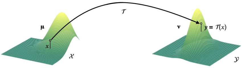
where T #µ denotes the measure image of µ by T , defined by : for all measurable subset B ⊂ Y,
T #µ(B) = µ(T −1 (B)) = µ({x ∈ X : T (x) ∈ B}). The condition T #µ = ν, models a local mass con-
servation constraint : the amount of masses received in any subset B ⊂ Y corresponds to what was transported here,
that is the amount of masses initially present in the pre-image T −1 (B) of B under T .

                            Figure 1: Monge’s problem. T is a transport map from X to Y

The solution to (M) might not exist because of the very restrictive local mass conservation constraint, it is the case, for
instance when µ is a Dirac mass and ν is not. One also remarks that (M) is rigid in the sense that all the mass at x must
be associated to the same target y = T (x). In fact, it is clear that if the mass splitting really occurs, which means that
there are multiple destinations for the mass at x, then this displacement cannot be described by a map T . Moreover, the
problem (M) is not symmetrical, the measures µ and ν do not play the same role, and this causes additional difficulties
when studying the existence of solutions for problem (M).

Kantorovich’s relaxed problem : The problem of Monge has stayed with no solution until 1942, when the
Soviet mathematician and economist Leonid Kantorovitch [26] suggested a convex relaxation of (M), which allows
mass splitting and guaranteed to have a solution under very general assumptions, this relaxed formulation is known as
the Monge-Kantorovich problem :
                                               Z
                                (MK) inf {           c(x, y) dγ(x, y) | γ ∈ Π(µ, ν) },                            (2)
                                            γ      X ×Y

where Π(µ, ν) is the set of transport plans constituted of all joint probability measures γ on X × Y with marginals µ
and ν :
                                Π(µ, ν) = {γ ∈ P(X × Y)|π1 #γ = µ and π2 #γ = ν}
π1 and π2 stand for the projection maps : π1 : X × Y → X        and π2 : X × Y → Y.
                                                (x, y) 7→ x               (x, y) 7→ y
The main idea of Kantorovich is to widen the very restrictive problem (M), instead of minimizing the total
cost of the transport according to the map T , it is towards probability measures over the product space X × Y that
Kantorovitch’s look turns to, these joint probability measures are a different way to describing the displacement of the
mass of µ : rather than specifying for each x ∈ X , the destination y = T (x) ∈ Y of the mass originally presented at
x, we specify for each pair (x, y) ∈ X × Y how much mass goes from x to y. Intuitively, the mass initially present
at x must correspond to the sum of the masses “leaving” from x during the transportation, and in a similar manner,
the finalRmass prescribed in y should
                                  R     correspond to the sum of the masses “arriving” in y, that can be written as :
µ(x) = Y dγ(x, y) and ν(y) = X dγ(x, y), which corresponds to a condition on the marginals : π1 #γ = µ, and
π2 #γ = ν, we are therefore now limited to working on measures whose marginals coincide with µ and ν : Π(µ, ν)
is then the admissible set of (MK). The relaxation of Kantorovitch is a much more suitable framework which
gives the possibility of mass splitting. Furthermore this relaxation has the virtue of guaranteeing the existence of
a solution under very general assumptions : X and Y are Polish spaces, and the cost function c is lower semi-continuous.

The Wasserstein distances : Whenever X = Y is equipped with a metric d, it is natural to use it as a cost
function, e.g. c(x, y) = d(x, y)p for p ∈ [1 , +∞[. In such case, the problem of Monge-Kantorovich defines a distance
between probability measures over X , called the p-Wasserstein distance, defined as follows :
                                                 Z
                          Wp (µ, ν) = inf (           dp (x, y) dγ(x, y))1/p , ∀µ, ν ∈ P(X )                      (3)
                                        γ∈Π(µ,ν)    X2

                                                            3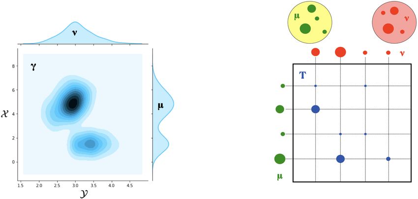
Figure 2: Continuous Kantorovich’s relaxation : the joint probability distribution γ is a transport plan between µ and ν
(left). Discrete Kantorovich’s relaxation : the positive entries of the discrete transport plan are displayed as blue disks
with radius proportional to the entries values (right)

The Wasserstein distance is a powerful tool to make meaningful comparisons between probability measures, even
when the supports of the measures do not overlap. This metric has several other advantages, first of all, they have an
intuitive formulation and they have the faculty to capture the underlying geometry of the measures by relying on the
cost function c = dp which encodes the geometry of the space X . The fact that the Wasserstein distance metrize weak
convergence is an other major advantage and makes it an ideal candidate for learning problems.

Discrete optimal transport : In applications, direct access to the measure µ and ν is often not available, in-
stead, we have only access to i.i.d. finite samples from µ and ν : X =P(x1 , ..., xn ) ⊂ X and YP= (y1 , ..., ym ) ⊂ X ,
                                                                          n                             m
in that case, these can be taken to be discrete measure : µ =             i=1 ai δxi and ν =            j=1 bj P
                                                                                                               δyj , where a
                                                                        P
and b are vectors in the probability simplex : a = (a1 , ..., an ) ∈        n and   b  = (b 1 , ..., b m ) ∈      m , where :
P             k
                                        Pk
   k = {u ∈ R | ∀i ≤ k, ui ≥ 0 and         i=1 ui = 1}. The pairwise costs can be compactly represented as an n × m
matrix MXY of pairwise distances between elements of X and Y raised to the power p :
                                         MXY = [d(xi , yj )p ]i,j ∈ Mn×m (R+ )

In this case, the p-Wasserstein distance becomes the pth root of the optimum of a network flow problem known as the
transportation problem [5], this is a parametric linear program on n × m variables, parameterized by two elements
: the matrix MXY , which acts as a cost parameter, and the transportation polytope U (a, b) which acts as a feasible
set, defined as the set of n × m non-negative matrices such that their row and column marginals are equal to a and b
respectively :
                               U (a, b) = {T ∈ Mn×m (R+ ) | T 1m = a and T T 1n = b}.
Let hA, BiF = trace(AT B) be the Frobenius dot-product of matrices, then Wpp (µ, ν) —the distance Wp (µ, ν) raised
to the power p— can be written as :
                                      Wpp (µ, ν) = min hT, MXY iF                                              (4)
                                                          T ∈U (a,b)

Note that if n = m, and, µ and ν are uniform measures, U (a, b) is then the Birkhoff polytope of size n, and the
solutions of Wpp (µ, ν), which lie in the corners of this polytope, are permutation matrices.

Discrete optimal transport defines a powerful framework to compare probability measures in a geometrically
faithful way. However, the impact of optimal transport in machine learning community has long been limited and
neglected in favor of simpler ϕ-divergences or MMD because of its computational and statistical burden. in fact,
optimal transport is too costly and suffers from the curse of dimensionality:
Optimal transport have a heavy computational price tag : discrete optimal transport is a linear program, and thus can be
solved with interior point methods using network flow solvers, but this problem scales cubically on the sample size, in
fact the computational complexity is O(n3 log(n)) when comparing two discrete measures of n points in a general
metric space [33], which is often prohibitive in practice.

                                                             4
Optimal transport suffers from the curse of dimensionality : considering a probability measure µ over Rd , and its
−1
empirical estimation µ̂n , we have E[Wp (µ, µ̂n )] = O(n d ) [49]. The empirical distribution µ̂n becomes less and less
representative as the dimension d of the ambient space Rd becomes large, so that in the convergence of µ̂n to µ̂ in
Wasserstein distance is slow.
Entropy-regularized optimal transport : Entropy-regularized optimal transport has recently emerged as a
solution to the computational issue of optimal transport [17], and to the sample complexity properties of its solutions
[22].
The entropy-regularized problem reads:
Z
inf c(x, y) dγ(x, y) + εH(γ), (5)
γ∈Π(µ,ν) X ×Y
log( dγ(x,y)
R
where H(γ) = X ×Y dxdy ) dγ(x, y) is the entropy of the transport plan γ.
The entropy-regularized version of the discrete optimal transport reads:
min hT, MXY iF − εH(T ), (6)
T ∈U (a,b)
Pn Pm
where H(T ) = − i=1 j=1 tij (log(tij ) − 1) is the entropy of T
The main idea is to use −H as a regularization function to obtain approximate solutions to the original trans-
port problem. The intuition behind this form of regularization is : since the cardinality of the nonzero elements of
the optimal transport plan T ∗ is at most m + n − 1 [11], one can look for a smoother version of the transport, thus
lowering its sparsity, by increasing its entropy.
The objective of the regularized optimal transport is an ε-strongly convex function, as the function H is 1-
strongly concave : its Hessian is ∂ 2 H(T ) = −diag( t1ij ) and tij ≤ 1. Then the regularized problem has a unique
optimal solution. Introducing the exponential scaling of the dual variables u = exp( αε ) and v = exp( βε ) as well as the
exponential scaling of the cost matrix K = exp( −MεXY ), the solution of the regularized optimal transport problem has
the form Tε = diag(u)Kdiag(v). The variables (u, v) must therefore satisfy : u (Kv) = a and v (K T u) = b,
where corresponds to entrywise multiplication of vectors. This problem is known in the numerical analysis
community as the matrix scaling problem, and can be solved efficiently via an iterative procedure : the Sinkhorn-Knopp
algorithm [27], which iteratively update u(l+1) = Kva(l) , and v (l+1) = K T ub(l+1) , initialized with an arbitrary positive
vector v (0) = 1m . Sinkhorn’s algorithm [17], is formally summarized in Algorithm 1 :
Algorithm 1: Sinkhorn’s algorithm for regularized optimal transport
Parameters :ε
Input :(xi )i=1,...,n , (yj )j=1,...,m , a, b
mi,j = kxi − yj k2 , ∀i, j ∈ {1, ..., n} × {1, ..., m}
K = exp(−MXY /ε)
Initialize v ← 1m
while not converged do
a
u ← Kv
v ← KbT u
end
return ti,j = ui Ki,j vj , ∀i, j ∈ {1, ..., n} × {1, ..., m}
Note that for a small regularization ε, the unique solution Tε of the regularized optimal transport problem converges
(with respect to the weak topology) to the optimal solution with maximal entropy within the set of all optimal solutions
of (MK) [34].
3 Semi-supervised learning
In traditional machine learning, a categorization has usually been made between two major tasks: supervised and
unsupervised learning. In supervised learning settings, algorithms make predictions on some previously unseen data
5points (test set) using statistical models trained on previously collected labeled data (training set). In unsupervised
learning settings, no specific labels are given, instead, one tries to infer some underlying structures (clusters) by relying
on some concept of similarity between data points, such that similar samples must be in the same cluster.
Semi-supervised learning (SSL) [54] is conceptually situated between supervised and unsupervised learning.
The goal of semi-supervised learning is to use the large amount of unlabelled instances, as well as a typically smaller
set of labelled data points, usually assumed to be sampled from the same or similar distributions, in order to improve the
performance that can be obtained either by discarding the unlabeled data and doing classification (supervised learning)
or by discarding the labels and doing clustering (unsupervised learning).
In semi-supervised learning settings, we are presented with a finite ordered set of l labelled data points
{(x1 , y1 ), ..., (xl , yl )}. Each object (xi , yi ) of this set consists of an data point xi from a given input space X , and
its corresponding label yi ∈ Y = {c1 , ..., cK }, where Y is a discrete label set composed by K classes. However, we
also have access to a larger collection of u data points {xl+1 , ..., xu }, whose labels are unknown. In the remainder,
we denote with XL and XU respectively the collection of labelled and unlabelled data points, and with YL the labels
corresponding to XL .
Nevertheless, semi-supervised algorithms work well only under a common assumption: the underlying marginal data
distribution P(X ) over the input space X contains information about the posterior distribution P(Y|X ) [45]. When
P(X ) contains no information about P(Y|X ), it is intrinsically inconceivable to improve the accuracy of predictions, in
fact, if the marginal data distribution do not influence the posterior distribution, it is inenvisageable to gain information
about P(Y|X ) despite the further knowledge on P(X ) provided by the additional unlabelled data, it might even happen
that using the unlabeled data degrades the prediction accuracy by misguiding the inference of P(Y|X ). Fortunately,
the previously mentioned assumption appears to be satisfied in most of traditional machine learning problems, as is
suggested by the successful application of semi-supervised learning methods in numerous real-world problems.
Nonetheless, the nature of the causal link between the marginal distribution P(X ) and the posterior distribu-
tion P(Y|X ) and the way of their interaction is not always the same. This has given rise to the semi-supervised learning
assumptions, which formalize the types of expected interaction [45]:
0
1. Smoothness assumption : For two data points x, x that are close in the input space X , the corresponding
0
labels y, y should be the same.
2. Low-density assumption : The decision boundary should preferably pass through low-density regions in the
input space X .
3. Manifold assumption : The high-dimensional input space X is constituted of multiple lower-dimensional
substructures known as manifolds and samples lying on the same manifold should have the same label.
4. Cluster assumption : Data points belonging to the same cluster are likely to have the same label.
According to the goal of the semi-supervised learning algorithms, we can differentiate between two categories :
Transductive and Inductive learning [45], which give rise to distinct optimization procedures. The former are solely
concerned with obtaining label predictions for the given unlabelled data points, whereas the latter attempt to infer a
good classification function that can estimate the label for any instance in the input space, even for previously unseen
data points.
The nature and the objective of transductive methods, make them inherently a perfect illustration of Vap-
nik’s principle: when trying to solve some problem, one should not solve a more difficult problem as an
intermediate step [13]. This principle naturally suggests finding a way to propagate information via direct connections
between samples by rising to a graph-based approach. If a graph can be defined in which similar samples are connected,
information can then be propagated along its edges. According to Vapnik’s principle, this method will allow us to avoid
the inference of a classifier on the entire input space and afterwards return the evaluations at the unlabelled points.
Graph-based semi-supervised learning methods generally involve three separate steps: graph creation, graph weighting
and label propagation. In the first step, vertices (representing instances) in the graph are connected to each other,
based on some similarity measure. In the second step, the resulting edges are weighted, yielding an affinity matrix,
such that, the stronger the similarity the higher the weight. The first two steps together are commonly referred to as
graph construction phase. Once the graph is constructed, it is used in the second phase of label propagation to obtain
predictions for the unlabelled data points [41]. The same already constructed graph will be used in inductive tasks to
predict the labels of previously unseen instances.
64 Proposed approach
4.1 Optimal Transport Propagation (OTP)
In this section we show how the transductive semi-supervised learning problem can be casted in a principally new way
and how can be solved using optimal transport theory.
Problem setup : Let X = {x1 , ..., xl+u } be a set of l + u data points in Rd and C = {c1 , ..., cK } a discrete label set
for K classes. The first l points denoted by XL = {x1 , ..., xl } ⊂ Rd are labeled according to YL = {y1 , ..., yl }, where
yi ∈ C for every i ∈ {1, ..., l}, and the remaining data points denoted by XU = {xl+1 , ..., xl+u } ⊂ Rd are unlabeled,
usually l
u.
The goal of transductive semi-supervised learning is to infer the true labels YU for the given unlabeled data
points using all instances in X = XL ∪ XU and labels YL .
To use optimal transport, we need to express the empirical distributions of XL and XU in the formalism of
discrete measures respectively as follows :
l
X l+u
X
µ= ai δxi and ν = bj δ x j . (7)
i=1 j=l+1
Emphasized that when the samples XL and XU are a collection of independent data points, the weights of all instances
in each sample are usually set to be equal :
1 1
ai = , ∀i ∈ {1, ..., l} and bj = , ∀j ∈ {l + 1, ..., l + u}. (8)
l u
Proposed approach : Transductive techniques typically use graph-based methods, the common denominator of
graph-based methods is the graph construction phase consisting of two steps, the first one lies to model the whole
dataset as a graph, where each data point is represented by a vertex, and then forming edges between vertices, and graph
weighting step, where a weight is associated with every edge in the graph to provide a measure of similarity between
the two vertices joining by each edge. Nonetheless, the most of graph construction methods are either heuristic or very
sophisticated, and do not take into account all the geometrical information in the input space. In this paper, we propose
a novel natural approach called Optimal Transport Propagation (OTP) to estimate YU , by constructing a complete
bipartite edge-weighted graph and then propagate labels through its vertices, which can be achieved in two phases:
Phase 1 : Construct a complete bipartite edge-weighted graph G = (V, E, W), where V = X is the vertex
set, that can be divided into two disjoint and independent parts L = XL and U = XU , E ⊂ {L × U } is the edge set,
and W ∈ Ml,u (R+ ) is the affinity matrix to denote the edges weights, the weight wi,j on edge ei,j ∈ E reflects the
degree of similarity between xi ∈ XL and xj ∈ XU .
The first difference we can notice between our label propagation approach and traditional ones is the type of
the graph G and the dimension of the affinity matrix W. Typically, traditional algorithms consider a fully connected
graph, that generates a square affinity matrix W, which could be very interesting in the framework of label noise
[41], i.e. if our goal is to label all the unlabeled instances, and possibly, under the label noise assumption, also to
re-label the labeled examples. However, the objective function of these traditional approaches penalize predicted
labels that do not match the correct label [45], in other words, for labelled data points, the predicted labels should
match the true ones, which makes the label noise assumption superfluous. Instead of this paradigm, we adopt
a complete bipartite edge-weighted graph [2], whose vertices can be divided into two disjoint sets, the first set
models the labelled data, and the second one, models the unlabelled data. Each edge of the graph has endpoints
on differing sets, i.e. there is no edge between two vertices of the same set, and every vertex of the first set is
connected to every vertex of the second one. This type of graph, naturally induces a rectangular affinity matrix, con-
taining less elements than the affinity matrix that one could have by considering a fully connected graph : l×u < (l+u)2 .
With regard to the graph construction, it must take into consideration that, intuitively, we want data points
that are close in the input space Rd to have similar labels (smoothness assumption), so we need to use some distance
that quantitatively defines the closeness between data points. Let MXL XU = (mi,j )1≤i≤l,l+1≤j≤l+u ∈ Ml,u (R+ )
denotes the matrix of pairwise squared distances between elements of XL and XU , defined by :
mi,j = kxi − xj k2 , ∀i, j ∈ {1, ..., l} × {l + 1, ..., l + u} (9)
7Since our approach satisfy the smoothness assumption, then any two instances that lie close together in the input space
Rd have the same label. Thus, in any densely area of Rd , all instances are expected to have the same label. Therefore, a
decision boundary can be constructed that passes only through low-density areas in Rd , thus satisfying the low-density
assumption as well.
Traditional label propagation approaches [53][52] create a fully connected weighted graph as mentioned ear-
lier, and a so-called affinity matrix W is used to denote all the edge weights based on the distance matrix and a Gaussian
kernel controlled by a free parameter σ, in the following way : an edge ei,j is weighted so that the closer the data points
xi and xj are, the larger the weight wi,j :
wi,j = exp(−kxi − xj k2 /2σ 2 ), ∀i, j ∈ {1, ..., l + u} (10)
Usually, σ is determined empirically. However, as mentioned by [52], it is hard to determine an optimal σ if only very
few labeled instances are available. Furthermore, even a small perturbation of σ, as pointed out by [48], could make the
classification results very different.
In [48], authors suggest to derive another way to construct the affinity matrix W, using the neighborhood in-
formation of each point instead of considering pairwise relationships as Eq(10). However, this approach presents two
issues : the first one resides in the assumption that all the neighborhoods are linear, Pin other words each data point
can be optimally reconstructed using a linear combination of its neighbors : xi = j/xj ∈N(x ) wi,j xj , where N(xi )
P i
represents the neighborhood of xi , and wi,j is the contribution of xj to xi , such that j∈N(x ) wi,j = 1 and wi,j ≥ 0,
i
but it is clear that this linearity assumption is unfortunately not always verified, moreover, the authors mention that
it is mainly for computational convenience, the second issue is the choice of the optimal number k of data points
constituting the linear neighborhood, typically k is selected by various heuristic techniques, however a variation of k
could make the classification results extremely divergent.
To overcome these issues, the new version of the label propagation algorithm proposed in this paper, at-
tempts to exploit all the information in X and the relations between labeled and unlabeled data points in a global
vision instead of the pairwise relationships or the local neighborhood information, and without using a Gaussian
Kernel. This faculty is ensured naturally by optimal transport, which is a powerful tool for capturing the underlying
geometry of the data, by relying on the cost matrix MXL XU which encodes the geometry of X. Since optimal transport
suffers from a computational burden, we can overcome this issue by using the entropy-regularized optimal transport
version that can be solved efficiently with Sinkhorn’s algorithm proposed in [17]. The regularized optimal plan
T ∗ = (ti,j )1≤i≤l,l+1≤j≤l+u ∈ Ml,u (R+ ) between the two measures µ and ν is the solution of the following problem :
T ∗ = argmin hT, MXL XU iF − εH(T ), (11)
T ∈U (a,b)
The optimal transport matrix T ∗ can be seen as a similarity matrix between the two parts L and U of the graph G,
in fact the elements of T ∗ provides us with the weights of associations with labeled and unlabelled data points. In
other words, the amount of masses ti,j flowing from the mass found at xi ∈ L toward xj ∈ U can be interpreted in our
label propagation context as the degree of similarity between xi and xj : similar labeled and unlabelled data points
correspond to higher value in T ∗ .
The advantage of our optimal transport similarity matrix is its ability to capture the geometry of the whole
X before assigning the weight ti,j to the pair (xi , xj ), unlike the similarity matrix constructed by the Gaussian kernel
that captures information in an bilateral level by considering only the pairwise relationships as [53][52], or in an local
level by considering the linear neighborhood information as [48], these two methods neglect the other interactions
which may occur between all the data points in X. This geometrical ability allows to the matrix T ∗ to contain mush
more information than the classical similarity matrices.
In order to have a class probability interpretation, we column-normalize T ∗ to get a non-square left-stochastic matrix
P = (pi,j )1≤i≤l,l+1≤j≤l+u ∈ Ml,u (R+ ), as follows :
ti,j
pi,j = P , ∀i, j ∈ {1, ..., l} × {l + 1, ..., l + u}. (12)
i ti,j
where pi,j , ∀i, j ∈ {1, ..., l} × {l + 1, ..., l + u} is then the probability of jumping from xi to xj . We consider P as
the affinity matrix W. Our intuition is to use this matrix to identify labelled data points who should spread their labels
to similar unlabelled data points in the second phase.
8Phase 2: Propagate labels from the labeled data XL to the remaining unlabeled data XU using the bipartite
edge-weighted graph constructed in the first phase. We will use an incremental approach to achieve this objective.
Let U = (uj,k )l+1≤j≤l+u,1≤k≤K ∈ Mu,K (R+ ) be a label matrix defined by :
X
uj,k = pi,j , ∀j, k ∈ {l + 1, ..., l + u} × {1, ..., K}. (13)
i/xi ∈ck
Note that U is by definition
P a non-square right-stochastic matrix, and can be understand as a vector-valued
function U : XU → K , which assigns a stochastic vector Uj to each unlabeled data point xj . Then for all
j ∈ {l + 1, ..., l + u}, xj have soft labels, which can be interpreted as a probability distribution over classes. The
choice of the construction of the matrix U in this way, follows the principle : the probability of an unlabeled data point
to belong to a class ck is proportional to its similarity with the representatives of this class. The more the similarity is
strong the more the probability of belonging to this class is high.
The label matrix U will be used to assign a pseudo label for each unlabeled data point in the following way
: ∀j ∈ {l + 1, ..., l + u}, xj will take the label corresponding to the class ck , k ∈ {1, ..., K}, which have the largest
class-probability uj,k of moving from all the data points belonging to ck toward xj .
yˆj = argmax uj,k , ∀j ∈ {l + 1, ..., l + u}. (14)
ck ∈C
Nevertheless, inferring pseudo-labels from matrix U by hard assignment according to Eq(14) in one fell swoop has a dis-
pleasing impact : we define pseudo-labels on all unlabeled data points whereas plainly we do not have a steady certainty
for each prediction. This effect, as pointed out by [24], can degrade the performance of the label propagation process.
To overcome this issue, we will assign to each pseudo-label yˆj a score sj ∈ [0, 1] reflecting the certainty of the prediction.
The certainty score sj associated with the label prediction yˆj of each data point xj ∈ XU can be constructed as follows
: for each unlabelled data point xj , we define a real-valued random variable Zj : C → R defined by Zj (ck ) = k, to
associate a numerical value k to the potential label prediction result ck . The probability distribution of the random
variable Zj is encoded in the stochastic vector Uj :
P(Zj = ck ) = uj,k , ∀j, k ∈ {l + 1, ..., l + u} × {1, ..., K} (15)
Then, the certainty score associated with each unlabelled data point can be defined as :
H(Zj )
sj = 1 − , ∀j ∈ {l + 1, ..., l + u} (16)
log2 (K)
where H is Shannon’s entropy [39], defined by :
X X
H(Zj ) = − P(Zj = ck ) log2 (P(Zj = ck )) = − uj,k log2 (uj,k ). (17)
k k
Since Shannon’s entropy H is an uncertainty measure that reach the maximum log2 (K) when all possible events are
1
equiprobable, i.e. P(Zj = ck ) = K , ∀k ∈ {1, ..., K} :
H(Zj ) = H(uj,1 , ..., uj,K ), ∀j ∈ {l + 1, ..., l + u}
1 1
≤ H( , ..., )
K K
X 1 1 (18)
=− log2 ( )
K K
k
= log2 (K)
Then, the certainty score sj is naturally normalized in [0, 1] as mentioned above.
To control the certainty of the propagation process, we define a confidence threshold α ∈ [0, 1], and for
each unlabelled data point xj , if the score sj is greater than α, we assign xj a pseudo-label yˆj according to Eq(14), and
then, we inject xj into XL , and yˆj into YL , otherwise, we maintains xj in XU . This procedure defines one iteration of
our incremental algorithm, in each of its iterations, we modify XL , YL and XU , in fact at each iteration, we increase
the size of XL , in return, the number of data points in XU decreases.
9The effectiveness of a label propagation algorithm depends on the amount of prior information, so enriching
XL at each iteration with new data points, will allow to the instances still in XU due to the lack of certainty in their
label predictions to be labeled, this time with greater certainty.
We repeat the same whole procedure until convergence, here convergence means that all the data initially in
XU are labelled during the incremental procedure.
The proposed algorithm, named OTP, is formally summarized in Algorithm 2.
Algorithm 2: OTP
Parameters :ε, α
Input :XL , XU , YL
while not converged do
Compute the cost matrix MXL XU by Eq(9)
Solve the regularized Optimal Transport problem in Eq(11)
Compute the affinity matrix P by Eq(12)
Get the label matrix U by Eq(13)
for xj ∈ XU do
Compute the certainty score sj by Eq(16)
if sj > α then
Get the pseudo label yˆj by Eq(14)
Inject xj in XL
Inject yˆj in YL
else
Maintain xj in XU
end
end
end
return YU
4.2 Convergence analysis of OTP
As mentioned earlier, the convergence of OTP means that all the data initially in XU are labelled during the incremental
procedure, i.e. when the set XL absorbs all the instances initially in XU , or in an equivalent way, when XU is reduced
to the empty set ∅. To analyze the convergence of our approach, we can formulate the evolution of XL and XU over
time, as follows :
Let mt be the size of the set XL at time (iteration) t, the evolution of mt is subject to the following nonlin-
ear dynamical system (R) :
mt = r(mt−1 ) = mt−1 + ζt
(R) : (19)
m0 = l
where ζt is the number of instances in XU that have been labeled during the iteration t. Since in an iteration t, we
can label all the instances in XU if the parameter α is P
too weak, or no point if α is very large, then the terms of the
sequence (ζt )t can vary between 0 and u, and we have t≥1 ζt = u.
Symmetrically, let nt be the size of the set XU at time t, this evolution is modeled by the following nonlin-
ear dynamical system (S) :
nt = s(nt−1 ) = nt−1 − ζt
(S) : (20)
n0 = u
From a theoretical
Pτ point of view, our algorithm OTP must converge at thePinstant t = τ , which verifies :
τ
mτ = m0 + t=1 ζt = m0 + u = l + u, which corresponds also to nτ = n0 − t=1 ζt = n0 − u = u − u = 0.
OTP will reach the instant τ in a finite number of iterations, in fact, experiments have shown that a suitable
choice of α will allow us to label a large amount ζt of samples in XU at each iteration t, otherwise, it suffices to
decrease α in the following way : suppose that at an iteration t, we have h unlabeled data points, whose certainty score
10Figure 3: Overview of the proposed approach. We initiate an incremental process where at each iteration we construct a
complete bipartite edge-weighted graph based on the optimal transport plan between the distribution of labelled data
points and unlabelled ones, then we propagate labels through the nodes of the graph, from labelled vertices to unlabelled
ones, after the evaluation of the certainty of the label predictions.
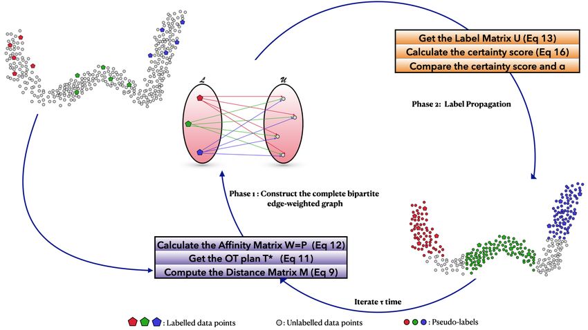
Figure 4: The evolution of the label propagation process (from the left to the right): at the initial iteration t = 0, at an
intermediate iteration 0 < t < τ , and at the last iteration t = τ . Pentagon markers correspond to the labeled instances
and circles correspond to the unlabeled ones which are gradually pseudo-labeled by OTP. The class is color-coded.
sj is lower than the threshold α, which means that none of these examples can be labeled according to OTP procedure
at the iteration t, the solution lies then in decreasing the value of α as follows :
α←α− min (α − sj ) (21)
xj ∈(XU )t
we denote by (XU )t the set of the h points constituting XU at iteration t. Decreasing the value of α in this way, will
allow to the point with the greatest certainty score in (XU )t to be labeled, and then to migrate from XU to XL .
Since integrating this point into XL can radically change in the next iteration the certainty scores of the
h − 1 data points that are still in XU , we can try to go back to the initial value of α, and essay to label normally the
h − 1 instances. Otherwise, if the problem persists, we can apply the same technique of decreasing α to label a new
point, and so on until convergence.
114.3 Induction for Out-of-Sample Data :
In the previous section we have introduced the main process of OTP, but it is just for the transductive task. In a truly
inductive setting, where new examples are given one after the other and a prediction must be given after each example,
the use of the transductive algorithm again to get a label prediction for the new instances is very computationally
costly, since it needs to be rerun in their entirety, which is unpleasant in many real-world problems, where on-the-fly
classification for previously unseen instances is indispensable.
In this section, we propose an efficient way to extend OTP for out-of-sample data. In fact, we will fix the
transductive predictions {yl+1 , ..., yl+u } and based on the objective function of our transductive algorithm OTP we will
try to extend the resulting graph to predict the label of previously unseen instances.
OTP approach can be casted as the minimization of the cost function CW,lu in terms of the label function
values at the unlabeled data points xj ∈ XU :
X X
CW,lu (f ) = wxi ,xj lu (yi , f (xj )) (22)
xi ∈XL xj ∈XU
where lu is an unsupervised loss function. The cost function in Eq(22) is a smoothness criterion that lies for penalizing
differences in the label predictions for connected data points in the graph, which means that a good classifying function
should not change too much between similar instances.
In order to transform the above transductive algorithm into function induction for out-of-sample data points,
we need to use the same type of smoothness criterion as before for a new testing instance xnew , and then we can
optimize the objective function with respect to only the predicted label f˜(xnew ) [4]. The smoothness criterion for a
new test point xnew becomes then :
X
C ∗ (f˜(xnew )) =
W,lu wx ,x lu (yi , f˜(xnew ))
i new (23)
xi ∈XL ∪XU
If the loss function lu is convex, e.g. lu = (yi − f˜(xnew ))2 , then the cost function CW,l
∗
u
is also convex in f˜(xnew ),
the label assignment f˜(xnew ) minimizing CW,lu is then given by :
∗
P
wxi ,xnew yi
f˜(xnew ) = Pxi ∈XL ∪XU (24)
xi ∈XL ∪XU wxi ,xnew
In a binary classification context where C = {+1, −1}, the classification problem is transformed into a regression one,
in a way that the predicted class of xnew is thus sign(f˜(xnew )).
It would be very interesting to see what happens when we apply the induction formula (Eq 24) on a point xi
of XU . Ideally, the induction formula must be consistent with the prediction get it by the transduction formula (Eq
22) for an instance xi ∈ XU . This is exactly the case in OTP, in fact, induction formula gives the same result as the
transduction one over unlabeled points : for xnew = xk , k ∈ {l + 1, ..., l + u}, we have :
∂C X
= −2 wi,k (yi − f (xk )) (25)
∂f (xk )
xi ∈XL
C is convex in f (xk ), and is minimized when :
P
wxi ,xk yi
f (xk ) = Pxi ∈XL
x ∈X wxi ,xk
P i L
wxi ,xk yi (26)
= Pxi ∈XL ∪XU since wxi ,xk = 0, ∀xi ∈ XU
xi ∈XL ∪XU wxi ,xk
= f˜(xk )
While the most of transductive algorithms have the ability to handle multiple classes, the inductive methods mostly only
work in the binary classification setting, where C = {+1, −1}. Following the same logic as [19], our optimal transport
approach can be adapted and extended accurately for multi-class settings, in the following way : the label f˜(xnew ) is
given by the weighted majority vote of the others data points in X = XL ∪ XU :
X
f˜(xnew ) = argmax wx ,x i new
(27)
ck ∈C
xi ∈XL ∪XU /yi =ck
12Our proposed algorithm for the inductive task called Optimal Transport Induction (OTI), is summarized in algorithm 3,
where we use the algorithm (OTP) for training and Eq(27) for testing.
Algorithm 3: OTI
Parameters :ε, α
Input :xnew , XL , XU , YL
(1) Training phase
Get YU by (OTP)
(2) Testing phase
For a new point xnew , compute its label f˜(xnew ) by Eq(27)
return f˜(xnew )
5 Experiments
5.1 Datasets
The experiment was designed to evaluate the proposed approach on 12 benchmark datasets, which can be downloaded
from 2 . Details of these datasets appear in Table 1.
Table 1: Experimental datasets
Datasets #Instances #Features #Classes
Iris 150 4 3
Wine 178 13 3
Heart 270 13 2
Ionosphere 351 34 2
Dermatology 366 33 6
Breast 569 31 2
WDBC 569 32 2
Isolet 1560 617 26
Waveform 5000 21 3
Digits 5620 64 10
Statlog 6435 36 6
MNIST 10000 784 10
5.2 Evaluation Measures
Three widely used evaluation measures were employed to evaluate the performance of the proposed approach: the
Accuracy (ACC) [29], the Normalized Mutual Information (NMI) [21], and the Adjusted Rand Index (ARI) [23].
• Accuracy (ACC) is the percentage of correctly classified samples, formally, accuracy has the following
definition:
Number of correct predictions
Accuracy = Total number of predictions
• Normalized Mutual Information (NMI) is a normalization of the Mutual Information (MI) score to scale the
results between 0 (no mutual information) and 1 (perfect correlation). In this function, mutual information is
normalized by some generalized mean of true labels Y and predicted labels Ŷ .
2I(Y,Ŷ )
N M I(Y, Ŷ ) = H(Y )+H(Ŷ )
information of Y and Ŷ , defined as: I(Y, Ŷ ) = H(Y ) − H(Y |Ŷ ) with H is the entropy
where I is the mutual P
defined by: H(Y ) = y p(y) log(p(y))
2
Datasets are available at https://archive.ics.uci.edu/
13• The rand index is a measure of the similarity between two partitions A and B, and is calculated as follows :
a+d
Rand(A, B) = a+b+c+d
where : a is the number of pairs of elements that are placed in the same cluster in A and in the same cluster in
B, b denotes the number of pairs of elements in the same cluster in A but not in the same cluster in B, c is
the number of pairs of elements in the same cluster in A but not in the same cluster in B and d denotes the
number of pairs of elements in different clusters in both partitions. The values a and d can be interpreted as
agreements, and b and c as disagreements.
The Rand index is then “adjusted for chance” into the ARI using the following scheme:
Rand−ExpectedRand
ARI = maxRand−ExpectedRand
The adjusted Rand index is thus ensured to have a value close to 0 for random labeling independently of the
number of clusters and samples and exactly 1 when the clustering are identical (up to a permutation).
5.3 Experimental protocol
The experiment compared the proposed algorithm with three semi-supervised approach, including LP [52] and LS [53],
which are the classical label propagation algorithms, LNP [48], which is an improved label propagation algorithm with
modified affinity matrix, and the spectral clustering algorithm SC [32] without prior information.
To compare these different algorithms, their related parameters were specified as follows :
• The number of clusters k for spectral clustering was set equal to the true number of classes on each dataset.
• Each of the compared algorithms LP, LS and NLP, require a Gaussian kernel controlled by a free parameter σ
to be specified to construct the affinity matrix, in the comparisons, each of these algorithms was tested with
different σ values, and its best result with the highest ACC, NMI and ARI values on the dataset was selected.
• The efficiency of a semi-supervised algorithm depends on the amount of prior information. Therefore, in the
experiment, the amount of prior information data was set to 15, 25, and 35 percent of the total number of data
points included in a dataset.
• The effectiveness of a semi-supervised approach depends also on the quality of prior information. Therefore, in
the experiment, given the amount of prior information, all the compared algorithms were run with 10 different
sets of prior information to compute the average results for ACC, NMI and ARI on each dataset.
• To give an overall vision of the best approach on all the datasets, we define the following score measurement :
P P erf (A ,D )
SCORE(Ai ) = j maxi P erf i(Aij,Dj )
where P erf indicates the performance according to one of the three evaluation measures above of each
approach Ai on each data-sets Dj .
5.4 Experimental results
Tables 2, 3 and 4 list the performance of the different algorithms on all the datasets. These comparisons indicate that
the proposed algorithm is superior to the spectral clustering algorithm, this suggests that prior information is able to
improve the label propagation effectiveness, this statement is also confirmed by the fact that given the datasets, all the
label propagation algorithms show a growth in their performance in parallel with the increase of the amount of prior
information. Furthermore, the tables show that the proposed approach is clearly more accurate than LP, LS, and NLP
on most tested datasets. However, on some datasets, OTP performed slightly less accurately than LP. The tables also
present the proposed score results of each algorithm, which show that the best score belongs to the proposed label
propagation approach based on optimal transport, followed by LS and LP.
To confirm the superiority of our algorithm over the compared approaches, and especially LP, we suggest to
use the Friedman test and Nemenyi test [20]. First, algorithms are ranked according to their performance on each
dataset, then there are as many rankings as their are datasets. The Friedman test is then conducted to test the
null-hypothesis under which all algorithms are equivalent, and in this case their average ranks should be the same. If
the null hypothesis is rejected, then the Nemenyi test will be performed. If the average ranks of two approaches differ
by at least the critical difference (CD), then it can be concluded that their performances are significantly different. In
the Friedman test, we set the significance level α = 0.05. Figure 5 shows a critical diagram representing a projection of
14average ranks of the algorithms on enumerated axis. The algorithms are ordered from left (the best) to the right (the
worst) and a thick line connects the groups of algorithms that are not significantly different (for the significance level
α = 5%). As shown in figure 5, OTP seem to achieve a big improvement over the other algorithms, in fact, for all
evaluation measures, the statistical hypothesis test shows that our approach is more efficient than the compared ones
and that the closest method is LS and then LP, which is normal, as both are label propagation approaches, followed by
LNP and finally spectral clustering.
To further highlight the improvement of performances provided by our approach, we are conducting a sensi-
tivity analysis using the Box-Whisker plots [44]. Box-Whisker plots are a non-parametric method to represent
graphically groups of numerical data through their quartiles, in ordre to study their distributional characteristics. In
figure 6, for each evaluation measure, Box-Whisker plots are drawn from the performance of our algorithm and the
compared ones over all the tested datasets. To begin with, performances are sorted. Then four equal sized groups
are made from the ordered scores. That is, 25% of all performances are placed in each group. The lines dividing the
groups are called quartiles, and the four groups are referred to as quartile groups. Usually we label these groups 1 to 4
starting at the bottom. In a Box-Whisker plot: the ends of the box are the upper and lower quartiles, so the box spans
the interquartile range, the median is marked by a vertical line inside the box, the whiskers are the two lines outside the
box that extend to the highest and lowest observations.
Sensitivity Box-Whisker plots represents a synthesis of the performances into five crucial pieces of informa-
tion identifiable at a glance: position measurement, dispersion, asymmetry and length of Whiskers. The position
measurement is characterized by the dividing line on the median . Dispersion is defined by the length of the
Box-Whiskers. Asymmetry is defined as the deviation of the median line from the centre of the Box-Whiskers from the
length of the box. The length of the Whiskers is the distance between the ends of the Whiskers in relation to the length
of the Box-Whiskers. Outliers are plotted as individual points.
Figure 6 confirms the already observed superiority of our algorithm over the others for the three evaluation
measures. Indeed, regarding accuracy, we note that the Box-Whisker plot corresponding to OTP is comparatively short,
this suggests that, overall, its performance on the different datasets have a high level of agreement with each other,
implying a stability comparable to that of LP and LS, and significantly better than that of LNP and SC. For NMI, the
Box-Whisker plot corresponding to our approach is much higher than that of LNP and SC, also noting the presence of
2 outliers for LP and LS, these outliers correspond to Heart and Ionosphere datasets, where both approaches have
achieved very low scores, on the other hand, there is an absence of outliers for OTP, these indicators confirm the
improvement in terms of NMI by our approach. Concerning ARI, we notice that the medians of LP, LS and OTP are all
at the same level, however the Box-Whisker plots for this methods show very different distributions of performances,
in fact, the Box-Whisker plot of OTP is comparatively short, implying the improvement of the performance of our
algorithm in term of ARI over the other methods and a better stability.
All the experimental analysis indicates then, that the performance of the proposed algorithm is higher than
the other label propagation algorithms. This result is mainly attributed to the ability of the proposed algorithm to capture
mush more information than the previous algorithms thanks to the enhanced affinity matrix constructed by optimal
transport. It is equally noteworthy that the effectiveness of the proposed algorithm lies in the fact that the incremental
process take advantage of the dependency of semi-supervised algorithms on the amount of prior information, then the
enrichment of the labelled set at each iteration with new data points, allows to the unlabelled instances to be labeled
with a high certainty, which explains the improvement provided by our approach. Another reason for the superiority of
OTP over the other algorithms is its capacity to control the certitude of the label predictions thanks to the certainty
score used, which allows instances to be labeled only if we have a high degree of prediction certainty.
15Table 2: Accuracy values for semi-supervised methods
Datasets Percent LP LS LNP OTP SC
15% 0.9437 0.9453 0.8852 0.9507
Iris 25% 0.9531 0.9540 0.9261 0.9610 0.7953
35% 0.9561 0.9571 0.9392 0.9796
15% 0.9296 0.9296 0.8462 0.9250
Wine 25% 0.9417 0.9417 0.8597 0.9343 0.8179
35% 0.9482 0.9482 0.8727 0.9388
15% 0.7261 0.7304 0.5683 0.7696
Heart 25% 0.7734 0.7833 0.6826 0.8424 0.3411
35% 0.8239 0.8352 0.7731 0.8693
15% 0.8300 0.8310 0.8051 0.8796
Ionosphere 25% 0.8439 0.8462 0.8146 0.8871 0.4461
35% 0.8458 0.8476 0.8293 0.8978
15% 0.9324 0.9327 0.8948 0.9488
Dermatology 25% 0.9438 0.9438 0.9163 0.9520 0.4943
35% 0.9536 0.9536 0.9428 0.9566
15% 0.9566 0.9566 0.9153 0.9587
Breast 25% 0.9578 0.9578 0.9296 0.9649 0.7830
35% 0.9649 0.9649 0.9427 0.9730
15% 1.0000 1.0000 0.9568 1.0000
WDBC 25% 1.0000 1.0000 0.9879 1.0000 0.9682
35% 1.0000 1.0000 0.9970 1.0000
15% 0.7558 0.7558 0.6519 0.7559
Isolet 25% 0.7782 0.7782 0.6908 0.7767 0.5385
35% 0.8077 0.8077 0.7249 0.8053
15% 0.8318 0.8334 0.7719 0.8469
Waveform 25% 0.8401 0.8419 0.7892 0.8504 0.3842
35% 0.8423 0.8425 0.8062 0.8599
15% 0.9589 0.9589 0.9363 0.9678
Digits 25% 0.9737 0.9737 0.9571 0.9774 0.7906
35% 0.9801 0.9801 0.9784 0.9827
15% 0.8740 0.8730 0.8249 0.8516
Statlog 25% 0.8779 0.8771 0.8371 0.8533 0.6516
35% 0.8831 0.8821 0.8474 0.8538
15% 0.9210 0.9218 0.8247 0.9421
MNIST 25% 0.9460 0.9451 0.8371 0.9540 0.5719
35% 0.9551 0.9571 0.8408 0.9632
ALL Datasets SCORE 35.4544 35.4975 33.3619 35.8855 8.1971
16Table 3: NMI values for semi-supervised methods
Datasets Percent LP LS LNP OTP SC
15% 0.8412 0.8442 0.7534 0.8447
Iris 25% 0.8584 0.8621 0.8269 0.8667 0.7980
35% 0.8621 0.8649 0.8314 0.8852
15% 0.7821 0.7821 0.6815 0.7384
Wine 25% 0.8127 0.8127 0.7573 0.7790 0.7808
35% 0.8289 0.8289 0.7897 0.7963
15% 0.1519 0.1575 0.1091 0.2181
Heart 25% 0.2291 0.2472 0.1432 0.3683 0.1880
35% 0.3313 0.3546 0.2718 0.4374
15% 0.3502 0.3535 0.3256 0.4676
Ionosphere 25% 0.3848 0.3911 0.3572 0.5000 0.2938
35% 0.3972 0.4014 0.3725 0.5383
15% 0.8770 0.8779 0.8349 0.8935
Dermatology 25% 0.8932 0.8932 0.8692 0.9033 0.6665
35% 0.9128 0.9128 0.8959 0.9164
15% 0.7340 0.7360 0.6971 0.7449
Breast 25% 0.7451 0.7465 0.7192 0.7550 0.6418
35% 0.7909 0.7909 0.7706 0.8106
15% 1.0000 1.0000 0.9049 1.0000
WDBC 25% 1.0000 1.0000 0.9347 1.0000 0.9163
35% 1.0000 1.0000 0.9715 1.0000
15% 0.7785 0.7785 0.7184 0.7657
Isolet 25% 0.7987 0.7987 0.7503 0.7852 0.7545
35% 0.8210 0.8210 0.7869 0.8077
15% 0.4950 0.5009 0.4628 0.5256
Waveform 25% 0.5124 0.5192 0.4763 0.5319 0.3646
35% 0.5192 0.5229 0.4807 0.5421
15% 0.9150 0.9150 0.8891 0.9290
Digits 25% 0.9443 0.9443 0.9268 0.9489 0.8483
35% 0.9570 0.9570 0.9318 0.9607
15% 0.7396 0.7383 0.6792 0.6753
Statlog 25% 0.7483 0.7477 0.6859 0.6800 0.6139
35% 0.7572 0.7571 0.6907 0.6821
15% 0.8019 0.8028 0.7759 0.8177
MNIST 25% 0.8389 0.8367 0.7931 0.8442 0.6321
35% 0.8542 0.8599 0.8136 0.8730
ALL Datasets SCORE 33.9980 34.2042 31.6326 35.5237 9.5770
17You can also read