Bootstrap method for the estimation of measurement uncertainty in spotted dual-color DNA microarrays
←
→
Page content transcription
If your browser does not render page correctly, please read the page content below
Anal Bioanal Chem (2007) 389:2125–2141
DOI 10.1007/s00216-007-1617-0

 ORIGINAL PAPER

Bootstrap method for the estimation of measurement
uncertainty in spotted dual-color DNA microarrays
Tobias K. Karakach & Robert M. Flight &
Peter D. Wentzell

Received: 10 July 2007 / Accepted: 7 September 2007 / Published online: 27 September 2007
# Springer-Verlag 2007

Abstract DNA microarrays permit the measurement of                    Introduction
gene expression across the entire genome of an organism,
but the quality of the thousands of measurements is highly            The introduction of DNA microarray technology in recent
variable. For spotted dual-color microarrays the situation            years has revolutionized the study of molecular cell biol-
is complicated by the use of ratio measurements. Studies              ogy, making it possible to assess genome-wide changes
have shown that measurement errors can be described by                in gene expression in a single experiment [1, 2]. In many
multiplicative and additive terms, with the latter dominating         ways, DNA microarrays approach an ideal analytical sensor
for low-intensity measurements. In this work, a measure-              array platform, exhibiting good specificity through selective
ment-error model is presented that partitions the variance            base pairing, high sensitivity through fluorescence mea-
into general experimental sources and sources associated              surements, and generally complete coverage of the analyte
with the calculation of the ratio from noisy pixel data.              domain in cases where the genome has been mapped. Des-
The former is described by a proportional (multiplicative)            pite their widespread use, however, there are still a number
structure, while the latter is estimated using a statistical          of challenges to be overcome if microarrays are to achieve
bootstrap method. The model is validated using simulations            their full potential [3]. These include issues related to ex-
and three experimental data sets. Monte-Carlo fits of the             perimental design, data quality, normalization, and data
model to data from duplicate experiments are excellent, but           analysis, among others. From the beginning, measurement
suggest that the bootstrap estimates, while proportionately           quality has been a particular focus of microarray research,
correct, may be underestimated. The bootstrap standard er-            since all conclusions are based on the reliability of the
ror estimates are particularly useful in determining the reli-        primary data. Typically, the quality of measurements can
ability of individual microarray spots without the need for           vary greatly across the spots on a DNA microarray due to
replicate spotting. This information can be used in screen-           variations in the amount of DNA spotted or hybridized,
ing or weighting the measurements.                                    changes in spot morphology, the presence of contaminants
                                                                      such as dust, and other factors. Therefore, an assessment of
Keywords DNA microarrays . Measurement errors .                       measurement error variance for individual spots is impor-
Bootstrap . Gene expression . Transcriptomics .                       tant for determining the utility of the calculated ratios. This
Measurement quality . Uncertainty estimation                          variance estimate can be used, for example, to filter mea-
                                                                      surements of low quality or to weight the measurements
                                                                      appropriately in subsequent data-analysis steps [4, 5].
                                                                         Although there are a variety of DNA microarray plat-
                                                                      forms in common use, one of the most widely employed for
                                                                      gene-expression studies is the spotted dual-color micro-
T. K. Karakach : R. M. Flight : P. D. Wentzell (*)
                                                                      array. With these arrays, the mRNA from expressed genes
Department of Chemistry, Dalhousie University,
Halifax, Nova Scotia B3H 4J3, Canada                                  is first extracted from two samples, which will be referred
e-mail: peter.wentzell@dal.ca                                         to here as the “test” and “reference” samples. For both sam-
2126                                                                                        Anal Bioanal Chem (2007) 389:2125–2141

ples, the mRNA is reverse transcribed to single-stranded            that uses biological replicates and then subtracts the com-
cDNA and labeled with a fluorescent dye. Different dyes,            bined effects of the other three terms from the overall
typically the cyanine dyes Cy3 (green) and Cy5 (red), are           variance.
used to label the test and the reference samples, which are             The second term on the right, σslide   2
                                                                                                                  , arises from the
then co-hybridized on the microarray, where each spot               technical variations from one microarray slide to another
contains DNA complementary to a specific cDNA sequence.             and includes sources of variability related to the preparation
For each spot, intensities measured for the two different           (extraction, labeling, hybridization) and normalization of
wavelength channels can be converted into a ratio (test/            the responses from the two channels. This contribution can
reference) that indicates (after appropriate normalization)         be evaluated through technical replication, i.e. replicated
when the expression of the corresponding gene is up or              microarrays for the same biological source material. This
down-regulated in the test sample relative to the reference         removes the contribution of σbiol   2
                                                                                                           , and the remaining two
sample. The statistical significance of such findings, how-         terms can be subtracted from the overall variance to give
ever, is critically dependent on the reliability of the measured    σslide
                                                                      2
                                                                           .
ratio, so the ability to estimate measurement uncertainty is            The third contribution, σspot
                                                                                                   2
                                                                                                      , is due to spot-to-spot varia-
essential.                                                          tions within a slide and is most easily assessed by spotting
   The purpose of the present work is to develop a boot-            replicate DNA material at several locations on one slide.
strap method for estimating the uncertainty in individual           Although the best estimates are obtained when replicate
ratio measurements on a microarray. In particular, the pro-         spots are distributed in a random fashion across the whole
posed method is used to estimate the component of the               slide, this design is not efficient from a microarray produc-
overall uncertainty that is derived from the measurement            tion perspective, so replicated spots often occur side-by-side.
process itself, that is, the part of the uncertainty arising from       The final term on the right-hand side of Eq. (1), σmeas
                                                                                                                              2
                                                                                                                                  , is
the calculation of a ratio from pixel intensities corrupted with    the one of particular interest to this work and relates to
instrument noise. For a given microarray spot, this compo-          the actual determination of the ratio from individual pixel
nent may be either a minor or major contributor to the overall      intensities on each of the two channels. Irrespective of the
uncertainty, and therefore its assessment is critical. The          other contributions to the overall variance, which can be
methods developed here are of greatest utility when there           regarded as systematic effects at this level, the error in the
is no replication of spots within a microarray design, but          ratio measurement will depend on factors such as the inten-
are generally useful in evaluating the reliability of spots in      sity and noise of the fluorescence signals, the morphology
any design.                                                         of the spot, the spatial alignment of the wavelength chan-
                                                                    nels, the manner of the ratio calculation, the background
                                                                    levels, and the presence of outlying pixels due to saturation
Background                                                          or contamination. Often, especially for low to moderate
                                                                    intensity signals, σmeas
                                                                                           2
                                                                                                is the dominant source of error
Measurement error models                                            variance, and therefore its assessment is extremely useful.
                                                                    This idea is illustrated in Fig. 1, which shows a map of
Measurement errors in spotted dual-color microarray experi-         pixel intensities for the red and green channels for two
ments can arise from a variety of sources and these can be          different spots. Both spots give essentially the same cal-
combined or decomposed in a number of different ways. One           culated ratio of unity, but given the high level of intensity
simple general representation is:                                   of signals for the spot on the left, the ratio calculated is
                                                                    expected to be much more precise than for the spot on
σR2 ¼ σbiol
       2
            þ σslide
               2
                     þ σspot
                        2
                             þ σmeas
                                2
                                                             ð1Þ    the right, where the intensities are near background noise.
                                                                    Because σmeas2
                                                                                     is defined according to the characteristics of
In this equation, σR2 represents the overall variance in the        an individual spot, by definition it cannot, strictly speaking,
ratio measurement for a given spot. The first term on               be determined through replication, since each spot will have
the right-hand side of the equation, σbiol2
                                             , represents the       its own unique features. In practice, a close approximation
biological variation of the system under study and, depend-         to σmeas2
                                                                                can be achieved from side-by-side replicates,
ing on the experiment, is often the largest component of the        assuming that the spot morphologies and other character-
overall variance. This component arises from the fact that          istics are very similar. This assumption is usually valid,
there is a natural variation in gene expression levels among        since side-by-side replicates would be printed with the
similar or identical organisms or populations due to differ-        same pin and have a high spatial and temporal correlation
ences in genetic makeup and/or environment, or due to               in the printing and hybridization process. Nevertheless,
simple stochastic effects. This part of the variance can be         exceptions can occur. Moreover, for reliable estimation of
determined experimentally through a simple nested design            the variance, several replicate spots should be printed for
Anal Bioanal Chem (2007) 389:2125–2141 2127
Fig. 1 Pixel intensity maps of
red and green channels for two
microarray spots, with combined
images inset. Note that both
spots give the same ratio mea-
surement, but the one on the
right would be expected to be
more uncertain
each gene, and this redundancy often runs counter to the are associated with σmeas
2
, since this contribution becomes
efficient use of limited space on the microarray. important for low-intensity signals, while the multiplicative
The measurement error characteristics of DNA micro- errors associated with the other three terms should dis-
arrays have been extensively studied in recent years and appear at low intensities. Therefore we can combine the
some fairly consistent properties have emerged that are first three terms in Eq. (1) into an uncertainty associated
reproducible across different laboratories and even different with the experiment, σexpt
2
as opposed to the measurement
platforms. Although a variety of different models have been step. This term will encompass the multiplicative error con-
proposed [6–12], it is generally observed that the intensities tribution, so we can write:
measured on each channel follow a mixed model with a
multiplicative and additive term, with the latter dominating σR2 ¼ σexpt
2
þ σmeas
2
¼ c2 R2 þ σmeas
2
ð4Þ
for low-intensity signals that become corrupted with back-
ground noise. Ideker et al. [7] expressed this model as: Here, R is the ratio and c is the proportionality constant for
the multiplicative error, i.e. the RSD for high-intensity
x ¼ mx þ mx "x þ d x ð2Þ measurements. Like the intensity models, the multiplicative
where x is the background-corrected signal intensity on a component of the error represented by c should be fixed for
given channel for a particular spot, μx represents the true a given slide, but unlike these models, the second term will
mean intensity, and ɛx and δx are normally distributed not be fixed, since it depends on how the individual mea-
random variables with zero means and standard deviations surement errors combine in the ratio calculation. Therefore,
of s "x and s dx . Rocke and Durbin [8] made somewhat dif- a method is needed to estimate σmeas2
for each spot.
ferent distributional assumptions and employed the model:
Current approaches
x ¼ m x ehx þ d x ð3Þ
where the definitions are the same and ηx is normally The measurement error model described above for ratio
distributed with a mean of zero and a standard deviation of measurements with spotted two-color microarrays presents
s hx . With these models, it is assumed that the model pa- some difficulties from a data-analysis perspective in that it
rameters (ɛ, δ, η) are constant for a given slide and a given leads to a heteroscedastic error structure, i.e. non-uniform
channel. For either model, when the additive error term (δx) error variance in the measurements. There are two compo-
is negligible, the errors in the intensities will be propor- nents to this problem. The first difficulty arises from the
tional to the signal magnitude, so the relative standard multiplicative component of the uncertainty in both the in-
deviation (RSD) of the measured intensities is expected to tensity and ratio measurement domains, which means larger
be constant. It is easily shown through propagation of errors uncertainties for larger measurements. A common approach
that, under these conditions, the RSD in the measured ratio to dealing with this problem in microarray data analysis is to
of the two channels is also constant. carry out a logarithmic transformation of the data. For purely
To reconcile these models with that given in Eq. (1), it proportional errors, it is easily shown by propagation of
can be assumed that the additive contributions to the error errors that a log transform will homogenize the error var-2128 Anal Bioanal Chem (2007) 389:2125–2141
iance, leading to a homoscedastic error structure that is Ratio calculation methods
statistically more tractable.
The second contributor to heteroscedasticity in the ratio An integral element in the statistical behavior of any ratio
measurement arises from the contribution of the σmeas 2
term. measurement will be the manner in which the ratio is
Often, this term will be negligible compared to the mul- computed from the raw data. The fundamental problem is
tiplicative error component, but when it is not (typically one of taking intensity measurements from (typically) a few
for low to moderate intensity signals) it can destroy the hundred pixels on two channels and computing a single
proportional error structure so that logarithmic transforms representative ratio of intensities. Complicating factors in-
are ineffective for homogenizing the variance. The most clude the fact that spots are rarely uniform, the pixels may
common way to treat this problem is to eliminate spots not be perfectly aligned, outliers may be present, and back-
where the σmeas2
term becomes a significant or dominant ground subtraction normally needs to be carried out. Five
contributor by flagging spots with low intensities or dubious methods are commonly employed for ratio calculation:
shapes as bad. This process is generally known as data
1. ratio of means,
filtering. A variety of strategies can be employed to this end,
2. ratio of medians,
the most basic being a visual inspection of the spots. This
3. mean of ratios,
process is labor-intensive, however, and quite subjective, so
4. median of ratios, and
a number of automated procedures based on various quality
5. regression.
measures have been proposed [13–22] for use independently
or in conjunction with manual methods. Although more These methods can be employed for both the foreground
efficient and objective than visual inspection, automated and the background regions, as designated by the gridding
procedures are less flexible and face the challenge of re- procedure.
ducing all of the contributors to poor spot quality to a One of the simplest and most popular methods for ratio
numerical indicator. Perhaps more importantly, data filter- calculation is the ratio-of-means method, where the mean of
ing methods result in a binary classification of good or bad, pixel intensities is calculated for each channel and, after
while measurement uncertainties follow a continuum of background subtraction, these are used to determine the
magnitudes. Setting an arbitrary threshold runs the risk of ratio. In essence, this method integrates the signal intensity
excluding measurements that may contain important infor- values across the spot and, in doing so, should have a good
mation or corrupting the data with excessive noise. Clearly, signal-to-noise ratio (S/N) and a low sensitivity to mor-
a method that could quantify the uncertainty associated with phology or small channel misalignment. The biggest draw-
each measured ratio would be useful. back to this method is a high sensitivity to outliers which
One strategy that has been suggested for estimation of can adversely affect the calculation of the mean.
measurement uncertainty in ratio calculations is propaga- Another widely used method is the ratio-of-medians, which
tion of errors [13, 14]. In principle, if one knows the un- is similar to the ratio-of-means except that the calculation is
certainties in the two intensities used to calculate the ratio, carried out using the median intensity on each channel. This
the uncertainty in the ratio is easily determined. In practice, approach is more robust in terms of sensitivity to outliers, but
however, models employed to do this are overly simplistic can be sensitive to spot morphology. Specifically, if a spot
and do not account for the complex correlation structures exhibits significant regions of low intensity, as can be the case
of the signals and noise in the pixelated data. Furthermore, for “doughnut” or “crescent” shaped spots, for example, there
reliable estimates of the measurement uncertainty for the is a good chance that the median intensities will fall in this
intensities are difficult to obtain. This is especially true for region. This can be a problem because low-intensity signals
background intensities, which are normally subtracted from are more likely to exhibit high noise.
the raw intensity values. For these reasons, error propaga- For the mean-of-ratios and median-of-ratios methods,
tion generally gives poor estimates of measurement noise intensity ratios are first calculated on a pixel-by-pixel basis
and has not been widely employed with microarrays. following background subtraction for each spot. The mean
Another approach that has been used with microarray data or median of these pixel ratios is then taken to be the spot
is the application of a variance stabilizing transformation, ratio, with the latter providing a more robust estimate. One
such as the generalized log transform [10, 23–25]. These appealing feature of this approach is the potential to
methods attempt to homogenize the variance while incorpo- evaluate the dispersion of the calculated ratios as an
rating both the multiplicative and additive terms. They re- estimate of uncertainty. In practice, however, if there are
quire some estimation of the transform parameters, however. significant variations in the pixel intensities included in the
Moreover, the implementation of any transform runs the risk calculations, the low intensity pixels will result in much
of altering the structure that was present in the original data, noisier ratios and so the uncertainty estimates may be high
which may be undesirable in certain applications [5]. and the ratio calculation may be unreliable.Anal Bioanal Chem (2007) 389:2125–2141 2129
The regression method for ratio determination is not as classical approaches are not practical. The possibility of
widely used as some of the other methods, but has certain extending the application of this method to estimate the
advantages and is the method employed in this work. With measurement uncertainty component for microarray spots,
this method, the intensities for pairs of pixels across a spot σmeas, as defined above, was therefore explored. In this
are plotted against one another. In principle, this should work, the bootstrap method was implemented in conjunc-
lead to a straight line with a slope equal to the ratio. In tion with the regression method of ratio calculation, but it
practice, orthogonal regression should be used instead of could equally be applied with other ratio-calculation
ordinary least squares (OLS), since errors are observed on methods also. In fact, Brody et al. [11] employed the
both axes (channels) and this can lead to problems for OLS bootstrap method with a median-of-ratios calculation, but
when high slopes are obtained. In addition, reliable did not carry out a rigorous evaluation of its reliability,
estimation requires some low-intensity pixels in order to providing data for only three genes. In the present work,
define the line. These can come from the edges of the interpretation of the regression parameters and their
foreground region or within the spot itself. The regression standard errors, in the context of two-color microarrays, is
method works best for spots which exhibit substantial that the slope corresponds to the ratio while the intercept
variation in intensity across the foreground region as relates to differential background for the two channels
opposed to a high degree of uniformity, but, in the authors’ underneath each spot. Emphasis here is placed on estimat-
experience, the former is more common than the latter. The ing the standard error of the ratio alone.
regression method is perhaps most similar to the ratio-of- The main idea behind the bootstrap is that many new
means method and, like that method, will be sensitive to samples (referred to as bootstrap samples) are “created”
outliers, especially for high leverage pixels. However, a from the original population by re-sampling (with replace-
subtle but important advantage of the regression method is ment), hence circumventing the need for extensive replica-
that it eliminates the need for background correction since tion. For example, given a spot with 300 pixels on both red
the intercept of the regression automatically accounts for and green channels, one draws a sub-population of 300
this. With other methods, background correction can pixels (referred to as a bootstrap sample) at random (with
present difficulties because it requires that a background replacement) from the initial or original population and
region of sufficient size be defined around the spot that carries out a regression using these pixels to obtain a slope
does not impinge on other spots, leading to irregularly (ratio) and intercept which are then stored. Note that,
shaped regions. The selection of background regions is although the bootstrap sample also contains 300 pixels,
algorithm-specific and often proprietary in commercial some of the pixels from the original population will be
software, so background intensities may not be very represented multiple times and others not at all. A second
reproducible from one package to the next. Moreover, there round of re-sampling from the original population is then
is always the risk that the calculated background is not carried out, followed by a regression to obtain a second
representative due to contamination or spatial variations in slope and intercept which are also stored. Figure 2 provides
the region of the spot. It has also been demonstrated [26] a conceptual illustration of this approach. This process is
that the background under the spot (spot-localized back- repeated as many times as necessary to obtain a reasonable
ground) may not be the same as the background around the estimate of the standard error in the parameter:
spot, leading to errors in the ratio calculation. To define the vffiffiffiffiffiffiffiffiffiffiffiffiffiffiffiffiffiffiffiffiffiffiffiffiffiffiffiffiffiffiffiffiffiffiffiffiffiffiffiffiffiffiffi
u B 2
background, the regression method requires only a few u 1 X
ðseÞB ¼ t b
q i b q ð5Þ
low-intensity pixels near or within the spot. In the latter B 1 i¼1
case, this method can, in principle, compensate for spot-
localized background effects. For these reasons, the In this equation, (se)B is the standard error estimate with B
regression method was chosen for the ratio calculation in bootstrap samples, b qi is the parameter estimate (slope) for
this work, but the methodology developed can also be the ith bootstrap sample, and b q is the mean parameter
applied to the other calculation methods. estimate for all of the bootstrap samples. The standard error
calculated in this way is taken to be an estimate of σmeas.
Bootstrap uncertainty estimates The measurement component of the variance, σmeas 2
, is
estimated by the bootstrap method for each individual spot.
Bootstrap methods are well established in statistics and This can then be combined with the multiplicative
engineering fields where they have mainly gained recogni- component of the variance, σexpt 2
, to give the overall error
tion and popularity as approaches for variance estimation in variance in the ratio. The multiplicative component, or
the absence of replicate data [27–29]. In statistics, boot- more specifically, the value of the proportionality constant c
strapping is widely used for estimating standard errors or in Eq. (4), should be the same for all spots on a given
confidence intervals for parameters in cases where the microarray. It should be possible to estimate this value from2130 Anal Bioanal Chem (2007) 389:2125–2141
Fig. 2 Conceptual illustration
of bootstrap procedure. The k
bootstrap samples are created
from the sampled population of
size N by extracting N measure-
ments at random (with replace-
ment) in each case. The
parameter b θ is the estimate of
the true population parameter, θ, Pick N points
and bθ1 ; :::; b
θk are the bootstrap
estimates of the parameter at random with
replacement
Sampled Population Bootstrap Samples
θ̂ θ̂1* θ̂2* θ̂3* θ̂B*
replicate experiments, especially if the estimation of σmeas
2
ranging from 1% to 50% were examined, and typical
enables elimination of spots where this component of the images for spots with 5% and 40% noise are shown in
noise dominates. Fig. 3c–f.
Experimental data sets
Experimental
Three experimental microarray data sets were employed in
Simulated data this work to try to validate the bootstrap error estimation
procedure. The first was part of a time-course study
Since perfect experimental replication of spots with exactly investigating exit from stationary phase by baker’s yeast,
the same characteristics is not possible, some validation of Saccharomyces cerevisiae. These data were collected in the
the bootstrap method was carried out using simulated laboratory of Professor Margaret Werner-Washburne (Uni-
microarray spots. As it is impossible to generate represen- versity of New Mexico, Albuquerque, NM, USA) and
tations of every possible spot morphology, two fairly involved approximately 6,300 yeast genes. A complete
common shapes were used as models. The noise-free discussion of these experiments has appeared elsewhere
intensity maps of these are shown in Fig. 3a and b. The [30]. The entire time course involved 19 microarrays, but
first model spot had a morphology which is characterized for the purposes of this work, the interest was in replicate
by somewhat uniform intensity, with sloping edges and a slides prepared at time points: 0, 1, 10, 20, and 35 min,
slant equal to about 40% of the maximum signal on the which allowed an assessment of the multiplicative contri-
plateau. The second model spot exhibited a doughnut shape butions to the uncertainty in the ratio. Duplicate slides were
typical of many microarray spots, with a center region that available for each of these time points, except time point 0
dropped to about 30% of the maximum signal around the where triplicate measurements were made. Duplicate slides
outside. In each case, the spots were generated on a 21×21 were hybridized and scanned by two different individuals
pixel grid and had no background present. For the and on different days, incorporating additional components
simulations, normally distributed random noise was as- in the experimental variability. In addition to the availabil-
sumed with a standard deviation of 100 intensity units. In a ity of multiple replicates, this experiment had some other
given simulation, noise was specified as a percentage of the features that were useful in this study. First, as a time-
maximum signal on the red channel, so the model spot course study, there was a wide range of ratios (unlike what
profile was scaled accordingly to give the appropriate would be anticipated for simple comparator experiments),
maximum for the error-free measurements on that channel. which allowed error models to be tested over a large span
The ratio (red/green) was taken to be 2, so the error-free of values. Second, due to slide production inexperience, the
spot image for the green channel was taken to be half that quality of these slides was not optimal and included an
of the red channel. To generate the simulated data, the noise extensive representation of different spot morphologies and
was added to the error-free spot images and the resulting qualities.
values were rounded to the nearest integer to simulate the The second data set employed was another time-course
effects of quantization noise introduced through digitiza- study involving the intraerythrocytic developmental cycle
tion, although these were expected to be small. Noise levels of the parasite Plasmodium falciparum, responsible for theAnal Bioanal Chem (2007) 389:2125–2141 2131
Fig. 3 Intensity maps of simu-
lated microarray spots. Two spot a b
morphologies were employed,
the uniform spot with a sloped
top (left) and the doughnut
shape (right). The noise-free
spots are shown in (a) and (b),
while (c) and (d) represent 5%
noise and (e) and (f) represent
40% noise on the red channel
c d
e f
majority of the cases of human malaria worldwide. This presented here, the side-by-side replicates were used to
data set has been widely studied as it was a contest data set obtain an experimental estimate of the measurement
for the CAMDA (Critical Assessment of Microarray Data) uncertainty.
Conference in 2004, and is publicly available. In this work
it will be referred to as the CAMDA data set. Experimental Ratio calculation
details are available in the original reference [31]. Briefly,
the transcriptome was measured at hourly intervals over a As already noted the regression ratio method was used to
48-h period for a total of 55 slides (including replicates) calculate the ratio, but additional details are provided here
with about 7,300 features each. A common reference was that are especially relevant for experimental measurements.
used for all of the measurements. Triplicate measurements The first step in the ratio calculation for a given spot was
were made for the first time point at 1 h, and duplicate extraction of the paired pixel intensities. This was done
measurements were made at 7, 11, 14, 18, 20, 27 and 31 h. using the spot location and size information in the “grid”
It was primarily these replicates that were used in this work. file. Pairs of pixels for which either channel was saturated
The third data set utilized microarrays from an experi- were then removed from this list. Next, the pairs containing
ment designed to study the development of the Atlantic upper fifth percentile of pixel intensities on each channel
halibut (Hippoglossus hippoglossus). This experiment was were also removed from the data set (five to ten percent of
conducted in the laboratory of Dr Susan Douglas at the pairs in total, depending on redundancy). This was done to
NRC Institute for Marine Biosciences in Halifax, Nova reduce the chances of retaining in the data set outliers
Scotia, Canada. The experiment involved triplicate hybrid- arising from dust spikes. The designation of the ninety-fifth
izations to measure gene expression in juvenile halibut at percentile was somewhat arbitrary, but seemed sufficient to
each of five developmental stages, for a total of 15 slides. eliminate most dust spikes without having a significant
Measurements were made against a common reference and effect on the regression. Depending on the characteristics of
each triplicate set included one dye swap. Each slide the slide, this number could be adjusted. Orthogonal
consisted of 38,500 spots which included four side-by-side regression [32] was then carried out on the remaining pairs
replicates for each of the 9,625 unique features. In the work of pixel intensities, extracting the slope as the spot ratio.2132 Anal Bioanal Chem (2007) 389:2125–2141
Results and discussion the bootstrap estimates also increases, as would be
expected. For the case of 40% noise in Fig. 4c and d, the
In order to gain confidence in the measurement uncertain- extent of variation in the standard deviation estimates is
ties calculated for the specific ratios, it was necessary to quite large, ranging between 0.2 (10% uncertainty in the
determine how accurately the bootstrap-calculated value of nominal ratio) to 1 (50% uncertainty). However, it is im-
σmeas
2
reflected the true uncertainty in the measurements. portant to recognize that the primary purpose of the boot-
This is difficult to do, since there is no way to generate strap estimation in this application is to obtain a rough
perfect experimental replicates of a given spot. In order to estimate of σmeas that can be used for data filtering and
provide some validation for the results obtained, three weighting, and not for rigorous statistical testing.
approaches were employed. First, simulated data were used An important consideration in the application of the
in which the spot morphology could be carefully controlled bootstrap method is the number of bootstrap samples used.
and reproduced. In the second approach, Monte-Carlo Errors in this procedure can be attributed to fundamental
modeling of data from the yeast and CAMDA microarrays statistical errors, which cannot be improved by increasing
was employed. Finally, side-by-side replicates of spots in the number of bootstrap samples, and “Monte-Carlo”
the halibut microarray were used to generate an experi- errors, which disappear as the number of samples goes to
mental estimate of σmeas
2
that could be directly compared to infinity. In this application, it is important to minimize
bootstrap estimates. variations in the estimates due to Monte-Carlo errors while
at the same time keeping the number of bootstrap samples
Simulated data low to minimize the computational time needed for thou-
sands of microarray spots. Figure 5 shows a plot of the
To evaluate the bootstrap method for the simulated micro- standard deviation in the standard error estimates and the
array spots shown in Fig. 3, an estimate of the “true” root mean square of the bias as a function of the number of
measurement uncertainty was first obtained for each spot/ bootstrap samples for the case of the uniform/sloped spot
noise-level combination. This was done by generating with 20% noise. To generate this plot, 100 runs were
1,000 replicate spots with different noise realizations, carried out at each level of bootstrap sampling (B) and the
followed by calculation of the red/green ratio for each of standard deviations of the measurement error estimates
these replicates. The standard deviation of these ratios was were recorded. This was repeated ten times at each level to
taken as the true value of σmeas. Following this, 100 give the mean and error bars shown in the plot. Similar
additional replicates were generated, each with a different calculations were carried out for the bias to evaluate its
noise realization. For each of these, bootstrap estimates of stability, except in this case a root-mean-square value was
σmeas were obtained based on 200 bootstrap samples. These calculated to account for its dispersion around zero rather
estimates are plotted for two noise levels (5% and 40%) and than around a mean. Although such a plot will vary some-
both spot morphologies in Fig. 4, along with the “true” what as conditions are changed, it was generally found that
value of σmeas (horizontal line). Also shown in each sub- both features leveled off fairly quickly above 100 bootstrap
figure is an estimate of the bias (dashed line) for each of the samples. For the algorithms used in this work, 200 boot-
100 cases. The bias is the deviation of the estimated ratio strap samples were used.
from the true value and can be estimated as: The validity of the results obtained from these simu-
lations is, of course, predicated on the assumption of inde-
ðbiasÞB ¼ b
q b
q ð6Þ pendent and uniform errors in the pixel intensities. Such an
assumption is not likely to be valid, but it is difficult to
Here, bq is the mean value of the ratio for the bootstrap develop models for pixel errors which would be accurate
samples and b q is the ratio estimated from the original and universal. A proportional or shot-noise error structure is
population. Since the bias relates to the accuracy of the reasonable, likely in combination with an additive contri-
ratio estimate, it should ideally be considerably smaller than bution. Correlated noise on adjacent pixels is also likely,
the standard error. Although a bias correction can be made including effects that may arise from slight channel
in the estimate of the uncertainty, this can also increase the misalignment. It is not possible to simulate all of these
variance in that estimate and such a correction was not scenarios, but a simple set of simulations was carried out
performed in this work. that included a proportional error term in addition to the
The results in Fig. 4 show good general agreement uniform noise. Results were essentially the same as those
between the bootstrap-estimated uncertainties and the shown in Fig. 4, although it was noticed that there was a
standard deviation in the ratio measurement as estimated slight bias in the estimate of the ratio, as might be antic-
from many replications. In all cases, the bias is compara- ipated. However, it is clear that a full validation of the
tively low. As the level of noise is increased, the variance in bootstrap approach needs to include testing with experi-Anal Bioanal Chem (2007) 389:2125–2141 2133
Fig. 4 Bootstrap estimates of 0.04 0.04
standard deviation in the ratio a b
measurement (R/G=2) for sim-
0.03 0.03
ulated microarray spots. The
Standard Deviation
horizontal line is the estimate of
the “true” standard deviation 0.02 0.02
based on 1,000 replicates of the
spot, the solid blue line is the
0.01 0.01
bootstrap estimate of the stan-
dard deviation for each of 100
replicates, and the dashed red 0 0
line is the corresponding esti-
mate of the bias. The panels on -0.01 -0.01
the left are for the uniform spot 0 20 40 60 80 100 0 20 40 60 80 100
1 1
with the sloped top and those on
the right are for the doughnut- c d
shaped spot. Plots (a) and (b) 0.8 0.8
Standard Deviation
correspond to 5% noise in the
red channel, while (c) and (d) 0.6 0.6
correspond to 40% noise
0.4 0.4
0.2 0.2
0 0
0 20 40 60 80 100 0 20 40 60 80 100
Run Number Run Number
mental data as well as simulated data. The next two sections served, allowing a variety of measurement conditions to be
address this issue. examined. Likewise, these microarrays exhibited spots of
varying intensity and quality, again permitting the robust-
Yeast microarray data ness of the model to be explored. Finally, replicate mea-
surements were conducted for a number of time points (0,
The microarray data from the yeast exit from stationary 1, 10, 20, and 35 min), allowing the experimental variance
phase time-course study was chosen for experimental to be assessed.
validation of the bootstrap method for a number of reasons. In the first part of this study, the use of the bootstrap-
First, since this was a time-course study involving large estimated σmeas for screening unreliable microarray spots
changes in gene expression relative to a common reference was investigated. To do this, ratios from duplicate micro-
(log-phase yeast cells) a wide range of ratios were ob- array experiments can be compared to one another in the
form of a log-log plot. Logarithmic plots are normally
preferred for such comparisons because the proportional
0.05
error structure commonly observed for microarrays reduces
Standard deviation of bootstrap to a uniform (homoscedastic) error structure upon logarith-
0.04 uncertainty estimates mic transformation. Ideally, if duplicate experiments were
Root mean square of bootstrap in perfect agreement, the log-ratio plot should be a straight
bias estimates line with a slope of unity and an intercept of zero. However,
SD/RMS
0.03
a non-zero intercept is often observed in these plots due to
a required normalization of the two experiments arising
0.02 from differences in laser intensity, detector sensitivity, dye
labeling efficiency, the amount of RNA extracted, and so
0.01 on. Moreover, experimental noise related to σexpt and σmeas
will cause deviations from the line, as will measurements
considered “bad” due to anomalous shape, background
0 problems, optical interferences, or other factors. By elim-
0 200 400 600 800 1000
Number of Bootstrap Replicates (B) inating spots with excessively high measurement variance,
Fig. 5 Effect of the number of bootstrap samples used (B) on the σmeas, the reliability and reproducibility of the spots that
precision of the bootstrap error estimate and the bias estimate remain should be improved.2134 Anal Bioanal Chem (2007) 389:2125–2141
To illustrate this, Fig. 6 shows log-ratio plots for dupli- similar in magnitude to the RSD expected for σexpt. This
cate microarray slides at time zero (other duplicate sets are censoring resulted in the retention of 5,463 spots. Of the
similar). Fig. 6a shows a plot where all of the points have 766 spots rejected on the basis of σmeas, 624 had been
been retained except for those with a negative ratio on flagged, representing 42.3% of the flagged spots. Figure 6c
either slide, which are obviously erroneous. This results in again shows significant improvement over Fig. 6a and has
the retention of 6,229 spots out of the original 6,307. The characteristics similar to Fig. 6b, although fewer spots have
line plotted through the points represents the best fit by been removed. By reducing the cutoff below 30%, the
orthogonal least squares and the slope of this line is given quality can be further improved, but with a commensurate
in the figure. It can be seen that using this very unrestrictive increase in the number of censored points.
filtering criterion results in a substantial spread in the ratios When both flags and measurement uncertainty are used
from the duplicate samples and an improved screening as censoring criteria in generating the log-ratio plot, as
method is desirable. shown in Fig. 6d, the number of spots is further reduced to
In Fig. 6b, spots that have been flagged by an operator as 4,612. In this case, all but a few of the extreme outlying
“bad” (on either slide) have been removed, reducing the points have been eliminated, resulting in greater reliability
number of spots to 4,754. This flagging is a manual and in the data.
subjective procedure that generally happens when spot It is clear from these observations that neither flagging
grids are set up for the microarray image. This can result in nor censoring on the basis of a 30% cutoff in σmeas results
censoring of spots because of unusual morphology, unreli- in the elimination of all of the unreliable microarray spots.
able background, smearing, interferences, or other reasons This is not unexpected, since flagging is subjective and
at the discretion of the operator. It is clear that this cen- prone to human error, while filtering on the basis of the
soring resulted in improved data quality and better cor- bootstrap-estimated σmeas does not necessarily capture all of
relation between the two experiments, although there still the undesirable spot characteristics, such as anomalous
appear to be some outlying points in the plot. background characteristics. In addition, it appears that flag-
In Fig. 6c, the operator flags were ignored and censoring ging may unnecessarily eliminate a substantial number of
was based solely on the value of the measurement un- spots with useful information. The best censoring strategy
certainty, σmeas, removing any spots where the relative would appear to be one with a combination of the two
standard deviation from this source (RSDmeas=σmeas/R) was methods, with a more relaxed flagging criterion to min-
greater than 30%. This cutoff was somewhat arbitrary, but imize the rejection of spots which may be valid. More
Fig. 6 Log-ratio plots for dupli-
10 6
cate slides at time zero in the a b
yeast data set with various cri-
4
teria used for screening mea-
surements: (a) only spots with 5
log2(R2)
2
ratios less than zero are re-
log2(R2)
moved, (b) spots with a ratio 0
less than zero and operator- 0
flagged spots are removed; (c) -2
spots with a ratio less than zero
or a bootstrap-estimated RSD -5 N = 6229 -4 N = 4754
greater than 30% are removed, Slope = 0.900 Slope = 0.898
and (d) spots meeting any of the -6
-5 0 5 10 -5 0 5 10
three criteria (ratio30%) are removed 6
c 6 d
4
4
2
2
log2(R2)
log2(R2)
0
0
-2
-2
-4 N = 5463 -4 N=4612
Slope = 0.904 Slope = 0.921
-6 -6
-5 0 5 10 -6 -4 -2 0 2 4 6 8
log2(R1) log2(R1)Anal Bioanal Chem (2007) 389:2125–2141 2135
specifically, the flagging strategy should not focus on spots log-ratio plot and the calculated value of c is still useful as a
with low intensities, which are likely to be detected through composite estimate. Figure 7b shows a histogram of the
σmeas, but rather on spots with anomalous characteristics absolute orthogonal residuals from Fig. 7a, which appear to
that may not be censored on the basis of measurement exhibit a high degree of normality. The half-Gaussian curve
uncertainty alone. overlaid on the histogram was obtained by minimizing the
If censoring on the basis of σmeas is carried further, it can χ2 value for count statistics. The value obtained for χ2 was
be argued that if only spots with a small RSDmeas are 29.2 with 29 degrees of freedom (30 bins), a value con-
retained, then the dominant source of error in those re- sistent with a normal distribution given the critical value of
maining spots should be σexpt, which should exhibit a pro- 42.6 (α=0.05). The estimated standard deviation of the
portional error structure. Figure 7a shows a log-ratio plot, residuals was 0.168, corresponding to a proportional error
again with time zero duplicates, where censoring is based contribution of 8.2% (c=0.082). This proportional error
on flags and RSDmeas > 5% (in this instance, the second structure is clearly visible in a ratio (instead of log-ratio)
criterion captures 98.4% of the flagged spots). This reduces plot of the censored measurements in Fig. 7c. This analysis
the number of spots to 1,294, but the figure clearly shows was carried out for all seven sets of duplicates and, although
the high correlation and a slope that is closer to the ideal of there was some variation in the number of outliers detected
unity at 0.969. Assuming σexpt follows a proportional error and the level of proportional noise observed, the general
structure (i.e. σexpt = cR as given in Eq. 4), then it can be behavior was very similar to the case shown.
shown by propagation of error that the logarithmic trans- If censoring to remove spots with a large σmeas reveals
formation of the ratio should lead to a uniform variance the proportional error structure, then, conversely, including
when σmeas can be ignored: those spots may degrade the normality of the residuals in
the log-ratio plots. This is the case as illustrated in Fig. 8a,
dðlog2 RÞ 2 2
σ ðlog2 RÞ ¼
2
σexpt which shows a histogram analogous to that in Fig. 7b, but
dR with the cutoff set to RSDmeas >50% (the Gaussian fit is
1 c2 shown in red). Although the visual quality of the fit does
¼ 2
c 2R 2 ¼ ð7Þ not appear to be much different here, the spread of the
R2 ðln 2Þ ðln 2Þ2
points is substantially larger (σresid =0.25) and the χ2 of 150
Based on this, and assuming that both microarray slides indicates a lack of fit to a normal distribution. This was the
have the same proportional error structure (i.e. the same typical trend for all of the duplicate pairs as indicated in
value of c), it can be shown that the orthogonal residuals of Fig. 8b, which shows that the χ2 values generally increase
the fit in Fig. 7a should be normally distributed with a as the RSDmeas cutoff value increases. This suggests that
standard deviation given by: increasing the proportion of ratios with a significant con-
pffiffiffi tribution from σmeas corrupts the proportional error structure
2c associated with σexpt, which is consistent with the error
s resid ¼ ð8Þ
ln 2 model.
In reality, there will likely be differences in the proportional Although this approach provides some support for the
error factor, c, from one slide to another, but this does not model and indicates that the bootstrap estimates are asso-
invalidate the normality of the observed residuals in the ciated with the pure measurement uncertainty, it does not
120 2
4 a b c
100
2 χ2 = 29.2 1.5
Number of Spots
Ratio on Slide 2
80
( ν = 29)
log2(R2)
0
60 σresid= 0.168 1
-2
40
0.5
-4 N = 1294 20
Slope = 0.969
-6 0 0
-5 0 5 0 0.1 0.2 0.3 0.4 0.5 0 0.5 1 1.5 2
log2(R1) Orthogonal Residual Ratio on Slide 1
Fig. 7 (a) Log-ratio plot for the yeast data in Fig. 6 with a bootstrap-estimated RSD cutoff of 5%. (b) Histogram of the orthogonal residuals from
the fit in (a) along with a fit to a Gaussian distribution. (c) Ratio plot of the data in (a) showing the proportional error structure of the ratios2136 Anal Bioanal Chem (2007) 389:2125–2141
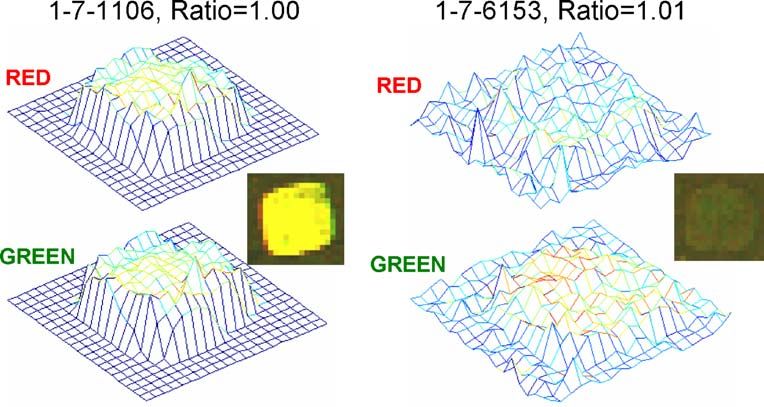
500 400
a b 1,2
350 1,3
400 Observed Residuals 2,3
300
Number of Spots
Gaussian Fit 4,5
Monte-Carlo Fit 250 7,8
χ 2 Value
300 10,11
200 14,15
200 150
100
100
50
0 0
0 0.2 0.4 0.6 0.8 1 0 10 20 30 40 50
Orthogonal Residual %RSDmeas Cutoff
Fig. 8 (a) Histogram of orthogonal residuals for the log-ratio plot of distribution of orthogonal residuals of log-ratio plots of duplicate
yeast time zero duplicates with a bootstrap-estimated RSD cutoff of yeast data sets to a Gaussian curve for various levels of RSD cutoff.
50%. The red line (plus symbols) shows a fit of the distribution to a The numbers in the legend refer to duplicate slide pairs. Note that the
Gaussian curve, while the blue line (crosses) is a Monte-Carlo fit of quality of the fit degrades as the cutoff is increased
the distribution to Eq. (10). (b) The χ2 values for fits of the
allow a direct quantitative and independent assessment of approach resulted in only a marginally improved fit with
σmeas. An indirect assessment is possible, however, through only a slightly lower χ2 value.
the use of Monte-Carlo simulations. Given a duplicate set It was postulated that the poor fit of the Monte-Carlo-
of slides with specified ratios and their associated errors, it simulated data might be the result of consistent under or
is possible to generate a set of simulated data with the same over-estimation of the bootstrap errors. Based on this,
distributional characteristics. To do this, projected ratios Eq. (9) was modified to include a scale factor adjustment
calculated from the linear fit of the log-ratio plot for a pair for the bootstrap error, designated as b in Eq. (10):
of slides were taken to be the “true” values. Simulated qffiffiffiffiffiffiffiffiffiffiffiffiffiffiffiffiffiffiffiffiffiffiffiffiffiffiffiffiffiffiffiffiffiffiffiffiffiffiffiffiffiffiffiffiffiffi
noisy measurements were obtained by adding normally σR ði; jÞ ¼ c 2 Rði; jÞ2 þ b 2 σboot 2 ði; jÞ ð10Þ
distributed random values to each set of “true” values. The
The optimization was then carried out to minimize the χ2
standard deviation associated with the error in each spot
value by adjustment of both b and c. This resulted in very
ratio was calculated from:
good fits of the observed distribution of orthogonal
qffiffiffiffiffiffiffiffiffiffiffiffiffiffiffiffiffiffiffiffiffiffiffiffiffiffiffiffiffiffiffiffiffiffiffiffiffiffiffiffiffi residuals to the distributions obtained from the Monte-
σR ði; jÞ ¼ c 2 Rði; jÞ2 þ σboot 2 ði; jÞ ð9Þ Carlo simulations, as shown by the blue curve in Fig. 8a.
These calculations were repeated for each of the duplicate
where σR(i,j) is the error standard deviation for spot j on slide sets in the data set and the results are summarized in
slide i, c is the proportional error component (RSD), R(i,j) Table 1, which includes the estimates of the proportional
is the estimated “true” ratio, and σboot is the bootstrap- error term (c), the scale factor for the bootstrap error (b), the
estimated measurement standard deviation. The simulated optimized χ2 value, and the uncertainties in each of these.
data generated in this way were carried through the same The parameters given are the mean values from five Monte-
calculations for the log-ratio plot as the experimental data, Carlo simulation runs with different random number seeds
using the same cutoff of 50% RSD for the bootstrap error and the uncertainties quoted are the corresponding standard
estimates. If the error model and bootstrap error estimates deviations.
are correct, this should lead to a distribution of residuals Table 1 reveals several interesting characteristics of the
that is similar to that for the experimental data. The two models. First of all, all of the χ2 values are quite rea-
distributions were compared using a χ2 statistic, which was sonable, well below critical values in most cases, and much
minimized by adjusting the value of the parameter c in improved over earlier models. This supports the validity of
Eq. (9); that is, the simulated (expected) distribution was the model used. The proportional errors extracted show a
fit to the experimental (observed) distribution by adjusting significant range over the set of duplicate slides, with a
the level of proportional error. To ensure reliability in the mean value around 14%. As already noted, these estimates
expected distribution, it was generated by calculating the assume that the proportional error contributions are the
average distribution of 50 sets of simulated measurements, same from each slide, although in reality this is not likely to
resulting in a relatively smooth curve. Unfortunately, this be the case, so the number is likely a root-mean-squareAnal Bioanal Chem (2007) 389:2125–2141 2137
Table 1 Results of Monte-Carlo fitting of orthogonal residuals for diminished, but some adjustment may be needed if a more
duplicate slide pairs in the yeast data set
quantitatively accurate estimate of the measurement uncer-
Time Slide % Proportional Scale factor χ2 tainty is required.
(min) pair error (100c) (b)
CAMDA microarray data
0 1,2 18.9±0.5 4.24±0.11 23.7±0.6
0 1,3 21.7±0.8 4.33±0.14 30.5±1.7
0 2,3 9.5±0.5 1.93±0.07 19.4±0.8 Given the somewhat unexpected results for the yeast micro-
1 4,5 37.2±1.6 3.61±0.40 44.0±2.5 array data, a second data set was investigated using the
10 7,8 0.14±0.11 4.20±0.04 57.2±1.6 same procedures. The Plasmodium falciparum time course
20 10,11 5.1±0.6 3.40±0.06 44.6±2.8 study available through the CAMDA project was a suitable
35 14,15 7.6±0.6 2.24±0.12 21.8±1.1 candidate because of its similarities to the yeast microarray
study. As for the yeast study, a wide range of ratios was
observed as a consequence of the large changes in gene
composite of the two contributions. The largest proportion- expression over time and replicate slides were available at
al error contribution is 37% observed for the duplicates at several time points, including triplicate measurements at the
1 min, which is not surprising since this is where the most first time point. Aside from these design similarities, how-
rapid changes in gene expression were observed to occur, ever, the two experiments were conducted in completely
likely leading to the poorest experimental reproducibility. separate laboratories using slides prepared on different micro-
What is quite surprising, however, is the very low pro- arrayers for different organisms.
portional error contribution for the measurements at 10 min. Despite the experimental differences between the two
Although this time point coincides with a relatively flat studies, the results obtained from the CAMDA data set
region for changes in gene expression, so a lower pro- were remarkably similar to those for the yeast and are only
portional error contribution might be anticipated, the virtual briefly summarized here. In terms of data filtering, the use
absence of any proportional error was quite unexpected. of flags or a 30% RSDmeas cutoff produced similar im-
Nevertheless, this result was very consistent and the fits provements in the log-ratio plots for duplicate slides, with
obtained were still quite satisfactory. fewer rejected measurements in the latter case. The best
Another surprising feature of the models is the magnitude results were obtained with the use of both criteria. These
of the scaling factors on the bootstrap estimates needed to observations are consistent with those made for the yeast
obtain a good fit. Although only minor adjustments with data set. When a cutoff of 3% RSDmeas was used, the pro-
values close to unity were anticipated, the values here range portional error structure became apparent, with a χ2 value
between about 2 and 4 with a mean of 3.4. To ensure that of 53.8 for a Gaussian fit to the orthogonal residuals of the
these estimates were not an algorithmic artifact, the fitting log-ratio plot for duplicates at the first time point (1,706
procedures were checked using simulated distributions and points retained). The cutoff for this set was lower than that
no significant bias was discovered. In addition, the distribu- used for the yeast data in Fig. 7a (5%) and the fit was not as
tion of the bootstrap estimates was examined for several good as in Fig. 7b because of the generally lower pro-
representative spots to check for skewness, but the distribu- portional error for these data (see below). At a 2% cutoff,
tions appeared symmetric with Gaussian character. The need the χ2 value was 34.2 (428 points retained) and at 5% it
for the scaling factor suggests that, although the bootstrap was 96.7 (3,990 points).
estimates were found to be accurate for the simulated spots Figure 9 is the CAMDA equivalent to Fig. 8 for the
described in the previous section, they are underestimated yeast data and employs duplicate measurements from the
by a factor of 2 to 4 for the experimental measurements, first time point. The histogram of the orthogonal residuals
indicating that there are some elements of the error structure when the cutoff was 50% RSDmeas shows a very poor fit
that were unaccounted for in the simulations. Nevertheless, it (red curve) to a Gaussian distribution, as expected, with a
was encouraging that a simple linear transformation was χ2 value of 726. As before, Fig. 9b shows that the quality
sufficient to provide a good fit to the observed distributions. of the Gaussian fit decreases as the cutoff is increased for
This is especially noteworthy for the duplicate slides at all replicate slide pairs. Also as before, the Monte-Carlo fit
10 min. Here the proportional error contribution is essential- to the observed distribution in Fig. 9a (blue curve) is much
ly zero, which means that the fit of the distribution is based improved over the Gaussian fit, with a χ2 value of 14.9.
almost solely on the bootstrap error estimates. Although the Table 2, which is equivalent to Table 1 for the yeast data,
χ2 value in this case is the highest in the group, the fit is shows the proportional errors and bootstrap error scaling
still remarkably good in the circumstances. This means that factors resulting from the Monte-Carlo fit for each of the
the utility of the bootstrap error estimates for distinguishing duplicate pairs in the CAMDA data set. As before, a range
reliable from unreliable measurements is not substantially of values was observed for both the proportional errorYou can also read