Profiling the Spatial Structure of London: From Individual Tweets to Aggregated Functional Zones
←
→
Page content transcription
If your browser does not render page correctly, please read the page content below
International Journal of
           Geo-Information

Article
Profiling the Spatial Structure of London: From
Individual Tweets to Aggregated Functional Zones
Chen Zhong 1 , Shi Zeng 2, * , Wei Tu 3                   and Mitsuo Yoshida 4
 1    Department of Geography, King’s College London, London WC2R 2LS, UK; chen.zhong@kcl.ac.uk
 2    Centre for Advanced Spatial Analysis, University College London, London WC1E 6BT, UK
 3    Key Laboratory of Spatial Information Smart Sensing and Services, School of Architecture and Urban
      Planning, Shenzhen University, Shenzhen 518060, China; tuwei@szu.edu.cn
 4    Department of Computer Science and Engineering, Toyohashi University of Technology, Toyohashi,
      Aichi 441-8580, Japan; yoshida@cs.tut.ac.jp
 *    Correspondence: shi.zeng.15@ucl.ac.uk; Tel.: +44-20-3108-3876

 Received: 21 August 2018; Accepted: 21 September 2018; Published: 25 September 2018

 Abstract: Knowledge discovery about people and cities from emerging location data has been
 an active research field but is still relatively unexplored. In recent years, a considerable amount
 of work has been developed around the use of social media data, most of which focusses on
 mining the content, with comparatively less attention given to the location information. Furthermore,
 what aggregated scale spatial patterns show still needs extensive discussion. This paper proposes
 a tweet-topic-function-structure framework to reveal spatial patterns from individual tweets at
 aggregated spatial levels, combining an unsupervised learning algorithm with spatial measures.
 Two-year geo-tweets collected in Greater London were analyzed as a demonstrator of the framework
 and as a case study. The results indicate, at a disaggregated level, that the distribution of topics
 possess a fair degree of spatial randomness related to tweeting behavior. When aggregating tweets
 by zones, the areas with the same topics form spatial clusters but of entangled urban functions.
 Furthermore, hierarchical clustering generates a clear spatial structure with orders of centers.
 Our work demonstrates that although uncertainties exist, geo-tweets should still be a useful resource
 for informing spatial planning, especially for the strategic planning of economic clusters.

 Keywords: geo-tweets; spatial structure; urban functions; clustering; topic modelling

1. Introduction
     Spatial planning and the allocation of urban resources (e.g., goods, infrastructure, services) need
to be supported by accurate and dynamic urban information. In recent years, emerging automatically
generated location data typified by smart card data, mobile phone data, and social media data has been
widely explored for applications such as, for instance, detecting events [1,2], extracting population
groups and their associated patterns [3,4], understanding human activity and mobility behaviors [5],
redrawing communities and boundaries [6–8], inferring activity types and land uses [9], evaluating
urban functionalities [10,11], and understanding the regularities of cities [12].
     This research considers tweets, an emerging location data set for understanding urban functionality
and spatial structure. As a social media system, Twitter allows registered users to share short text
messages, which are called tweets. There are 330 million average Monthly Active Users (MAUs)
according to the most recent annual report by Twitter showing a continued growth in recent years [13].
Compared to other urban mobility datasets, Twitter data is open to the public (in particular by
using standard streaming API with “locations” parameter), and highly available in most cities.
The data contains rich textual information and the near real-time nature is not available in other

ISPRS Int. J. Geo-Inf. 2018, 7, 386; doi:10.3390/ijgi7100386                        www.mdpi.com/journal/ijgi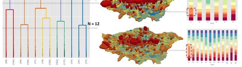
ISPRS Int. J. Geo-Inf. 2018, 7, 386                                                               2 of 14

populated datasets. Seeing the advantages, Twitter data has attracted considerable attention from
scientific communities. However, most of the previous work concerns the analysis of the tweets’
microblog content. The potential around location information needs more active exploration [14,15].
For applications in urban analytics specifically, on the one hand, massive progress has been made
using various types of emerging location data. On the other hand, a growing number of discussions
have pointed out the drawbacks and consequences rooted in the nature of automatic data—the lack
of demographic and contextual information [16,17], and the bias in sampling [18]. This leads to the
salient research question behind our work: with inferred information, at what aggregated level can
clear and meaningful spatial patterns be detected using geo-tweets in the context of urban analysis?
     Therefore, we proposed a multilevel analytical framework named as tweet-topic-function-structure
(TTFS) to reveal spatial patterns from individual levels at aggregated spatial scales, integrating
an unsupervised learning algorithm with spatial measures. A composite score is proposed to select
the best topic model as a base for the follow-up analysis. We applied the framework to a case study
of two-year geo-tweets collected in the Greater London Area (GLA). The analytical results fulfil our
two-fold research goals. Firstly, the multilevel analysis allows us to test our hypothesis that although
the spatial distribution of individual tweets in topics demonstrates degrees of randomness; collective
effects at an aggregated level show spatial clusters that correlate with entangled urban functions,
which at the city-wide level, enable us to extract a hierarchical spatial structure. Secondly, this work
profiles the functionality and structure of the GLA using Twitter data as a proxy, which contributes to
a better understanding of the social dynamics in the GLA. In sum, our work explored the potential of
Twitter data in informing spatial planning.

Related Work—Mining Spatial Patterns from Geo-Tweets
     Twitter users can opt in to geotag their tweets. From a random sampling of collected tweets
only 1% are geotagged. These statistics are in line with the other findings [19–21], even though,
previous work has proved the performance and functionality of geo-tweets in outlining dynamic
urban space. For instance, in [22], tweets in 39 countries were investigated. In particular, they found
a positive correlation between the number of tweets on the road and the Average Annual Daily Traffic
on highways in France and the UK. In developing countries, such as Kenya, as showcased in [23],
tweets have a good coverage across the entire country and could be used as an alternative source of
information for estimating flows of people. This paper positions tweets as a type of emerging big human
mobility data [24] and explores their potential in the field of urban analytics. A literature review is
therefore scoped accordingly. Apart from the works rooted in technical advances, e.g., data mining and
machine learning algorithms, previous related research around urban analytics may be summarized
into three categories.
     The first category of research makes best use of the rich textual information. The microblog
system delivers messages in natural language that allows us to understand people’s response to
the environment and events. For instance, tweets regarding a new Bus Rapid Transit system were
extracted and analyzed as an alternative source of understanding user satisfaction [25]. Geo-tweet
adds a spatial-temporal dimension to the analysis of perception. It has frequently been applied to
model the spreading impacts of emergency situations such as that exemplified by [2,26,27]. For this
sort of analysis, the results are comparatively promising as Hashtags were used to filter tweets into
themes and contribute a better interpretation of the contents.
     The second category gives more focus on the locational rather than contextual information,
mostly using spatiotemporal analysis. Steiger, Albuquerque and Zipf [15] did a systematic review
and found that although the number of publications around tweets increased dramatically, only 13%
of them focus on location information, and even fewer on specific applications. Visual analytics is
undoubtedly an important sub-category as shown by the spatiotemporal visualization framework used
in [28,29]. In addition, applications regarding human mobility and migration patterns have become
an important trend. For example, travel behavior was extracted from geo-tweets in Austria and Florida,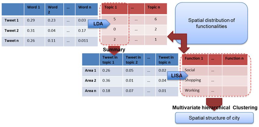
ISPRS Int. J. Geo-Inf. 2018, 7, 386                                                                   3 of 14

but with a focus on terrestrial long-distance travel only (that which extends over 100 km) [5]. Similarly,
long-distance movements were explored in [23]. Furthermore, clustering methods incorporating
spatial, temporal, and textual information have been widely applied to infer activity types or travel
purpose and segment user groups at an aggregated scale [30,31]. Results were generally verified with
travel surveys or census data [9,32], and it was concluded that working and commercially related
tweets or topics gave a better estimate. For long-term and even larger spatial scale movement patterns,
analysis around migration was explored, such as that in [33,34]. Although significantly limited by the
sample size of valid tweets, long-term historical tweets data is still useful for exploratory analysis and
inferring trends.
     The third category emphasizes urban morphology and system dynamics. It overlaps with the
two previous categories. Twitter data has been used to redraw the boundaries and landscapes in
social space, rather than physical geographical space [35]. In another work developed by Longley and
Adnan [36], demographic information was also inferred from tweets user profiles and combined with
land-use data to conduct a geo-demographic classification of the GLA. In [10], a quantitative measure
was proposed implementing Jane Jacobs’ concept of diversity and vitality and used Twitter as a proxy
for urban activities. Similarly, location-based check-in data have been used to infer place significance
and assess functional connectivity [11]. Our work aligns with this category but emphasizes spatial
structure on top of multilevel analysis.
     There is, in fact, a fourth area of enquiry, relating to the above three, which looks beyond the use
of tweet data, at all emerging mobility data types, and this remains an area of longer-term interest for
our work. This category investigates the uncertainties in the detected phenomena, in the methods
adopted, and in the tweet data itself. For instance, [37] discussed the similarities of patterns across
temporal, geographical and semantic characteristics in tweets data. Jurdak, et al. [38] found similar
overall features exist in mobile data and geo-tweets. They also reported variability caused by regular
and irregular users and animalized movements. In fact, the same issues were observed in other types
of mobility data [12,39]. Discussions around regularity and variability were initiated a while ago
with open questions posted. For instance, is there a universal pattern in mobility regardless of urban
context [40,41]? Are there limits in predicting mobility [42,43]? A discussion of this topic, with materials
drawn from our analysis, is touched upon in the last section.

2. Materials and Methods

2.1. Data and the Study Area
      The Twitter data for this study were sourced using a standard Twitter streaming API between
June 2015 and June 2017. The Twitter API provides a free and straightforward way to query a portion
of streaming tweets and returns results in a JavaScript Object Notation (JSON) format. The analysis
used geo-tweets only. Geo-tweets refer to those that have valid coordinates while excluding those
having a location tag only. Basic figures are given in Table 1.
      Four steps of data cleaning were conducted. The first three steps follow a generic preliminary
data processing that remove outliers by conditions. The last step is to prepare the data for text mining
with commonly used packages, i.e., re and Gensim. First, only tweets with coordinates falling in the
GLA were kept. Second, tweet accounts that posted an anomalous number of tweets greater than
average by a standard deviation were removed, as these are likely to be fake users or commercial
accounts. Third, tweet accounts that kept on posting at repeating coordinates were deleted, as these
are usually official accounts such as weather broadcasting. After these three steps, the distribution of
tweets per user id shows an exponential-like decay distribution without a long tail. Manual checking
was conducted for sampled tweets by user ids to verify our data cleaning process. The last step is
text cleaning for topic modelling. Tweets with fewer than four words were removed because they are
too short and do not contribute any meaningful content but instead, may bias the results. It is worth
mentioning that a phrase detection process was applied to automatically detect common phrases as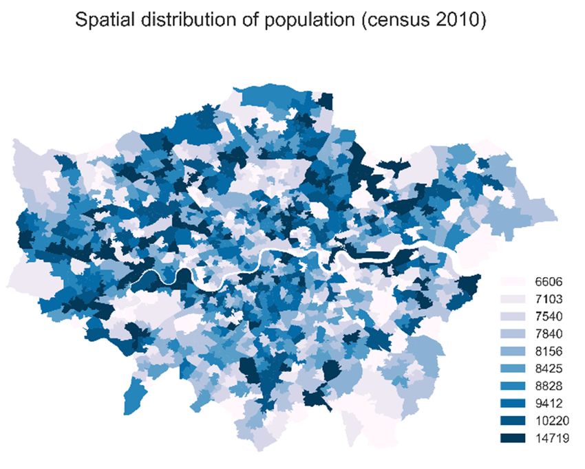
ISPRS Int. J. Geo-Inf. 2018, 7, 386 4 of 14
a step in the text clean-up. This combines words and forms phrases especially for location names,
for instance, “greater_london_area” is a combination of three words. We found that forming phrases
decreases the bias in analysis caused by frequent repeating words, such as “great” (which is the root
ISPRS Int. J. Geo‐Inf. 2018, 7, x FOR PEER REVIEW
of greater). 4 of 14
Table
Table 1.
1. Tweets
Tweets data
data from
from June
June 2015–June
2015–June 2017.
2017.
Number
Number of of Number of Avg.Tweets
Avg. Tweets
PerPer
Data
DataProcessing
Processing Number of Users
Tweets
Tweets Users User_id
User_id
1. All geo‐tweets
1. All geo-tweetscollected
collectedininGLA
GLA 6,647,704
6,647,704 483,444
483,444 1313
2. Remove
2. Remove repeating ids
repeating ids 4,166,542
4,166,542 481,007
481,007 99
3. Remove
3. Remove repeating
repeating coordinates
coordinates 2,275,852
2,275,852 326,218
326,218 77
4. Remove tweets with fewer than 4 words
4. Remove tweets with fewer than 4 words 1,938,275 288,603 7
(after cleaning up text) 1,938,275 288,603 7
(after cleaning up text)
Our analysis
Our analysisaimsaimsatatincluding
includinga afull
full spectrum
spectrum of of urban
urban functions.
functions. Therefore,
Therefore, all valid
all valid tweets
tweets are
are included in the analysis regardless of the time and frequency of tweeting. Geospatial
included in the analysis regardless of the time and frequency of tweeting. Geospatial data at Middle data at
MiddleSuper
Layer LayerOutput
Super Output Area (MSOA)
Area (MSOA) level used
level were were used for summarizing
for summarizing and and mapping
mapping (as (as shown
shown in
in Figure 1 left). The average population of an MSOA in London in 2010
Figure 1 left). The average population of an MSOA in London in 2010 was 8346. We chose to was 8346. We chose to use
use
MSOA level
MSOA level because
because it it gives
gives an
an adequate
adequate spatial
spatial resolution
resolution (938
(938 zones
zones for
for the
the GLA)
GLA) while
while at
at the
the same
same
time avoiding null values. As shown in Figure 1 right, there were no single zones without
time avoiding null values. As shown in Figure 1 right, there were no single zones without geo‐tweets. geo-tweets.
Figure
Figure 1.
1. Spatial
Spatial distribution
distribution of
of population
population (left)
(left) and
and geo‐tweets
geo-tweets in
in zones
zones (right).
(right).
2.2. Methodology
2.2. Methodology
We intentionally
We intentionallymademadethe theframework
framework moremore generic
generic by using
by using well-established
well‐established methods
methods (e.g.,
(e.g., Latent
Latent Dirichlet
Dirichlet Allocation
Allocation (LDA),(LDA), Multivariate
Multivariate Clustering)
Clustering) to ensure
to ensure such asuch a framework
framework can be can be
easily
adapted to other case studies across different fields. A comparative study is the next step to verify to
easily adapted to other case studies across different fields. A comparative study is the next step if
verify
the if the gained
insights insightsingained in this
this work work
can can contribute
contribute to othertourban
othercontexts.
urban contexts.
The twoThe two subsections
subsections below
below present
present the mostthe critical
most critical elements
elements in our
in our methodology:
methodology: (1) (1)
thethe workflow;
workflow; and(2)
and (2)an
an additional
additional
indicator for model selection for the research of urban spatial
indicator for model selection for the research of urban spatial patterns. patterns.
2.2.1. Framework—Tweets-Theme-Function-Structure (TTFS)
2.2.1. Framework—Tweets‐Theme‐Function‐Structure (TTFS)
We proposed a three-step framework that infers urban information from geo-tweets as that
We proposed a three‐step framework that infers urban information from geo‐tweets as that
shown in Figure 2 (step 1–3 is denoted from top to bottom). The first step is topic modelling of
shown in Figure 2 (step 1–3 is denoted from top to bottom). The first step is topic modelling of tweets
tweets and interpreting meaning of topics in urban context. For implementation, we use the Mallet
and interpreting meaning of topics in urban context. For implementation, we use the Mallet Java topic
Java topic modelling toolkit re-developed by Gensim with a python wrapper [44]. The way we
modelling toolkit re‐developed by Gensim with a python wrapper [44]. The way we select the best
select the best number of topics is detailed in Section 3.2. The second step is a summary analysis
number of topics is detailed in Section 3.2. The second step is a summary analysis along with a
qualitative interpretation of each topic and its projected urban functions. Local spatial autocorrelation
measures by Pysal [45] were applied to extract and analyze spatial clusters. In particular, local
indicators of spatial association (LISA) were applied, which identify hot spots that reflect
heterogeneities and contribute to global patterns [46]. The third step is multivariate hierarchical
clustering using the distribution of topics in each zone as vectors of input data. For instance, if there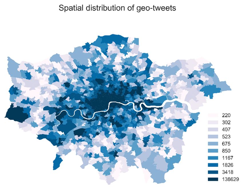
ISPRS Int. J. Geo-Inf. 2018, 7, 386                                                                        5 of 14

along with a qualitative interpretation of each topic and its projected urban functions. Local spatial
autocorrelation measures by Pysal [45] were applied to extract and analyze spatial clusters. In particular,
local indicators of spatial association (LISA) were applied, which identify hot spots that reflect
heterogeneities
ISPRS Int. J. Geo‐Inf. and   contribute
                       2018, 7, x FOR PEERto global patterns [46]. The third step is multivariate hierarchical
                                           REVIEW                                                          5 of 14
clustering using the distribution of topics in each zone as vectors of input data. For instance, if there
are T topics defined in step 1. The vectors used for spatial  spatial clustering
                                                                      clustering in
                                                                                 in step
                                                                                    step 3 will be a vector of T
variables. A spatial structure is expected to be identified after classifying zones into different
                                                                                               different groups.

        Figure 2.
        Figure    TTFS Framework
               2. TTFS Framework for
                                 for profiling
                                     profiling urban
                                               urban functionality
                                                     functionality and
                                                                   and structure
                                                                       structure from
                                                                                 from geotagged
                                                                                      geotagged tweets.
                                                                                                tweets.
2.2.2. Indicators for Select the Number of Topics
2.2.2. Indicators for Select the Number of Topics
      To extract information from our textual data, we applied one of the most prevalent topic modelling
      To extract information from our textual data, we applied one of the most prevalent topic
approaches—Latent Dirichlet Allocation [47]. LDA assumes each document in a corpus contains
modelling approaches—Latent Dirichlet Allocation [47]. LDA assumes each document in a corpus
numerous latent topics and each word is drawn from one of those topics. During calculation, each word
contains numerous latent topics and each word is drawn from one of those topics. During calculation,
is considered to be a vector, and each topic is a unique word probability distribution, and similar
each word is considered to be a vector, and each topic is a unique word probability distribution, and
semantic information will be grouped by underlying mathematical techniques. A generally agreed
similar semantic information will be grouped by underlying mathematical techniques. A generally
challenge of topic modelling is the interpretation of topics, which matters to the selection of the most
agreed challenge of topic modelling is the interpretation of topics, which matters to the selection of
optimal topic model. In this study, it is crucial because the detected topics define base urban functions
the most optimal topic model. In this study, it is crucial because the detected topics define base urban
for follow-up analysis. A commonly adopted way to select the best topic model is by coherence value,
functions for follow‐up analysis. A commonly adopted way to select the best topic model is by
which measures the quality of individual topics [48]. In general, the higher the coherence value,
coherence value, which measures the quality of individual topics [48]. In general, the higher the
the better the quality of the topics. We implemented a grid search of best topic models and ended up
coherence value, the better the quality of the topics. We implemented a grid search of best topic
with the same conclusion as that in [49]. Increasing the number of topics (T) leads to higher coherence
models and ended up with the same conclusion as that in [49]. Increasing the number of topics (T)
values. However, the higher value does not always mean the most meaningful value. Bringing too
leads to higher coherence values. However, the higher value does not always mean the most
many topics for an in-depth review of topics is not the focus of this research and gives no help to the
meaningful value. Bringing too many topics for an in‐depth review of topics is not the focus of this
distinguishing between urban functions and the associated spatial patterns. As a trade-off, on top of
research and gives no help to the distinguishing between urban functions and the associated spatial
coherence value, we added a global spatial autocorrelation measure, which involves the study of the
patterns. As a trade‐off, on top of coherence value, we added a global spatial autocorrelation measure,
distribution over the entire area and sees if the distribution displays clustering or not. We chose the
which involves the study of the distribution over the entire area and sees if the distribution displays
topic models that generate good spatial clusters, as it is generally known that urban agglomeration
clustering or not. We chose the topic models that generate good spatial clusters, as it is generally
happens as a natural process. For that spatial autocorrelation calculation, Moran’s I [50] is applied with
known that urban agglomeration happens as a natural process. For that spatial autocorrelation
the distribution of tweets in topics used as input vectors. To be more specific, if nine topics (t = 9) were
calculation, Moran’s I [50] is applied with the distribution of tweets in topics used as input vectors.
used, nine autocorrelations will be calculated, and we take the average value. To avoid any bias caused
To be more specific, if nine topics (t = 9) were used, nine autocorrelations will be calculated, and we
by the uneven distribution of tweets (as shown in Figure 1 right, a significant number of tweets were
take the average value. To avoid any bias caused by the uneven distribution of tweets (as shown in
concentrated in inner London area), the distribution of tweets in topics are normalized by each zone.
Figure 1 right, a significant number of tweets were concentrated in inner London area), the
distribution of tweets in topics are normalized by each zone.

3. Results
    The presentation of results is structured in line with the workflow presented in Section 3.1 along
with technical details. They are, moreover, aligned with the three subsections discussing the results
generated in this work and related to the discussion of urban mobility related literature. The focus is
multifold. First, it introduces a measure to quantify the general challenge of topic modelling, topic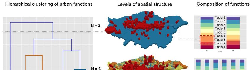
ISPRS Int. J. Geo-Inf. 2018, 7, 386                                                                  6 of 14

3. Results
     The presentation of results is structured in line with the workflow presented in Section 3.1 along
with technical details. They are, moreover, aligned with the three subsections discussing the results
generated in this work and related to the discussion of urban mobility related literature. The focus
is multifold. First, it introduces a measure to quantify the general challenge of topic modelling,
topic number t. Second, we demonstrate a spatial autocorrelation analysis to infer hot spots and
structure with the topics which we labelled. Last, we construct a framework which reveals the spatial
structure based on topics and functions, as well as the underlying correlations with other urban
theories or models.

3.1. Inferring Activity Types and Entangled Urban Functions
      The optimal topic model was selected with nine topics identified using coherence values and
an average spatial autocorrelation measure. In general, the coherence values increased along with the
number of topics as aforementioned. The result is in line with that in the data mining literature [49].
Conversely, the mean value of spatial autocorrelation decreased. This indicates the spatial distribution
is exhibiting higher levels of randomness, which makes the classification and interpretation of topics
more complicated when considering its associated spatial patterns. Therefore, topic model with
nine topics was selected as shown in Figure 3 (vertical line) as a trade-off between coherence and
autocorrelation values.
      Table 2 lists the clustered nine topics, the representative words in each topic, and the mapping
from words to topics and to their associated urban functions. The mapping is merely a qualitative
analysis process. As one way of verification, the detected keywords are closely related to those
identified in previous work [35,37]. Therefore, when defining the topics as activities, we referred to the
labels defined in related work. The classification of urban functions is related to the National Land Use
Classification in the UK [51], in which, 13 main land uses are defined along with a decomposition into
several sub-types. When mapping these activities to urban functions, we found it is not possible to
make a 1-to-1 mapping, because the labelled activities (column 2, topic) could happen in more than
one urban functional area. This revealed the shortcomings and the research potential for classifying
land use in functionally complicated urban area. One exception is topic 6—food and drink—which is
a straightforward case and is closely associated with the function of retail. The other topics all exhibits
a 1-to-N relationship. For instance, topic 5 routine activities are a high-level classification composed
of work, education, residential, etc., as we can identify from the keywords. The corresponding
urban functions could be residential, office, education, as well as people tweeting on their way
to their destinations; City hub is equivalent to multifunctional zones that attract large volumes of
flow population. The places identified in the keyword include critical transport hubs and popular
tourist sites.
      It is also worth noticing that the even distribution of topics given in the last column of the
table—the ratio of tweets in the topic—is quite unlike the statistical distribution of trip purpose gained
through official travel demand surveys or inferred activities from other mobility datasets, such as
smart card data [52]. In these, commuting trips have much higher occurrences in urban travel than
indicated in our Twitter data. This indicates the limits of using tweets for travel demand prediction.
The underlying reason for this could be the motivation for tweeting which will be further discussed
and the intermittent absence of mobile signal, such as that experienced in the London Underground,
resulting in data uncertainty.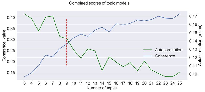
through official travel demand surveys or inferred activities from other mobility datasets, such as
smart card data [52]. In these, commuting trips have much higher occurrences in urban travel than
indicated in our Twitter data. This indicates the limits of using tweets for travel demand prediction.
The underlying reason for this could be the motivation for tweeting which will be further discussed
and the
ISPRS Int. intermittent
J. Geo-Inf. 2018, absence
7, 386 of mobile signal, such as that experienced in the London Underground,
7 of 14
resulting in data uncertainty.
ISPRS Int. J. Geo‐Inf.Figure
2018, 7,3.
Figure Selection
3.x FOR PEERof
Selection the
the best
REVIEW
of best number
number of
of topics
topics for
for unveiling
unveiling spatial
spatial patterns.
patterns. 7 of 14
3.2. Unveiling
3.2. Unveiling Collective
Collective Patterns
Patterns from
from Randomness
Randomness through
through aa Spatial
Spatial Clustering
Clustering of
of Functional
Functional Zones
Zones
From the
From the entangled urban functions
entangled urban functions embedded
embedded in in tweets,
tweets, we
we conclude
conclude that,that, rather
rather than
than taking
taking
modelled topics
modelled topics ofof the
the tweet
tweetasasaadefined
definedfunctionality
functionalityofofspace,
space,ititisismore
morereasonable
reasonabletototake
takeit it
asasa
a layer of probability from which we may infer spatial distributions
layer of probability from which we may infer spatial distributions and hotspots. and hotspots.
In the
In the second
second step, spatial correlation
step, spatial correlation analysis
analysis waswas applied.
applied. A A spatial
spatial weight
weight matrix
matrix waswas
constructed using
constructed using aa K K nearest
nearest neighborhood
neighborhood (KNN)(KNN) method
method with
with K K set
set to
to be
be 10.
10. Our
Our experiment
experiment
showed that choices of alternative K would only smooth the spatial distribution to aa certain
showed that choices of alternative K would only smooth the spatial distribution to certain degree,
degree,
but it
but it made
made no no dramatic
dramaticchange
changetotothetheobserved
observedoverall
overalltrend.
trend.Noting
Noting that
that thethe index
index of of
thethe matrix
matrix in
Figure 4 corresponds to the identification of topics in Table 2 we see that the non‐diagonal cellscells
in Figure 4 corresponds to the identification of topics in Table 2 we see that the non-diagonal are
are bivariate
bivariate spatial
spatial correlation
correlation of two
of two different
different topics.
topics. A higher
A higher value value
means means the distribution
the distribution oftwo
of the the
two topics
topics is likely
is likely to change
to change accordingly
accordingly in in space.
space. Overall,
Overall, lowbivariate
low bivariatecorrelations
correlationswerewere observed,
observed,
which is indicative of a spatially stable classification of
which is indicative of a spatially stable classification of topics.topics.
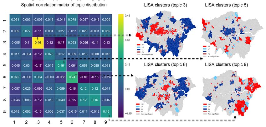
Figure 4.
Figure Local spatial
4. Local spatial autocorrelation
autocorrelation matrix
matrix (left)
(left) and
and maps
maps hotspot
hotspot of
of selected
selected topics
topics (right).
(right).ISPRS Int. J. Geo-Inf. 2018, 7, 386 8 of 14
Table 2. An interpretation of words in topics and responding urban functions.
c Topic Words in the Topic Urban Functions Moran’s I Ratio _tw (%)
Beautiful, make, studio, check, shoot, summer, light, photo, shop, art, gorgeous,
1 Fashion and arts top, hair, style, colour, beauty, wear, design, hand, eye, blue, set, exhibition, piece, Recreation and leisure/retail 0.051 11.94
store, black, project, perfect, collection
Time, tonight, show, year, today, start, ready, friday, tomorrow, party, open,
Recreation and
2 Events Christmas, week, book, event, Saturday, weekend, free, visit, end, part, join, 0.077 10.31
leisure/community services
finally, wait, leave, month, bring, ill, launch, excited
London, greater_london, city, hotel, covent_garden, station, england,
london_underground_station, bridge, victoria, good_morn, central, royal, tower,
Recreation and
3 City hub canary_wharf, westminster, kings_cross, tube_station, mayfair, hyde_park, soho, 0.46 15.34
leisure/Retails/Transport
kensington, leicester_square, wembley, hospital, united_kingdom, notting_hill,
camden_town, platform
Posted_photo, house, bar, place, park, street, view, road, garden, pub, cafe, pic,
4 Sight and view soho, market, theatre, centre, spot, town, shoreditch, east, camden, south, room, Recreation and leisure/Retail 0.078 12.14
local, pretty, chelsea, queen, dog, church, west
Today, day, work, back, morning, home, run, nice, feel, week, session, walk, bit,
Residential/Industry and
5 Routine activities post, sunday, long, class, train, office, sun, hour, finish, gym, Monday, training, 0.16 10.03
business/ transport
start, break, hard, early, follow
Drink, lunch, food, coffee, restaurant, breakfast, dinner, beer, eat, special, cocktail,
6 Food and drink delicious, brunch, drinking, green, cake, red, tea, wine, treat, hot, burger, fresh, Retail 0.24 11.17
taste, perfect, meal, chocolate, sweet, chicken, serve
Business People, life, thing, make, give, talk, bad, world, call, find, change, support, service,
Industry and
7 information, read, woman, job, share, learn, high, lose, business, point, story, word, stop, 0.12 10.03
business/transport/educational
networking student, plan, group, idea
Big, watch, live, play, man, club, boy, game, music, miss, face, school, film, turn,
Residential/Recreation and
8 Watch head, baby, moment, kid, video, dream, world, heart, picture, win, star, dance, 0.16 9.55
leisure
listen, fuck, king, rock
Good, great, love, day, night, amazing, lovely, last_night, happy, evening, team,
Recreation and
9 Socializing yesterday, friend, girl, fun, meet, guy, birthday, catch, awesome, enjoy, wonderful, 0.16 9.48
leisure/community services
weekend, lot, celebrate, happy_birthday, afternoon, family, lady, hopeISPRS Int. J. Geo-Inf. 2018, 7, 386 9 of 14
The diagonal of the matrix is the spatial autocorrelation of each topic distribution. In general,
values above 0 indicate trends of spatial clustering, with 1 indicating strong clustering, and below
0 meaning degrees of randomness. The autocorrelation values, though all above 0, do not exhibit
a strong clustering effect, overall. It is not a surprising result since the distribution of dominant
topics in zones does not give any clear spatial partition in GLA. In other words, any topic could be
tweeted anywhere in the city, suggesting that spatial dimension is not the most important factor in
tweeting behavior. Nevertheless, comparatively higher autocorrelations of some topics were obtained
as expected. For instance, City hub (Topic 3) shows the most significant hotspots of big hubs in GLA
that loosely connected from the west end to the north-west (Wembley), expanding to canary wharf and
the city airport, and areas near Heathrow airport. Most popular catering (topic 6) areas are concentrated
near to the central area. There is a partition of east/south London (Bromley and Havering borough)
to the rest of the area in the spatial distribution of topic 9, which can be explained as social activities
with family and friends mostly happening locally and in residential areas. These two boroughs are
likely to function as relatively more self-sufficient communities. Not all spatial clusters are so easily
interpreted in relation to topics. For instance, topic 5, does not generate either a big hotspot in inner
London representing working places, or widely distributed small hotspots representing residential
areas. Overall, we conclude that dominant topics characterize urban space only at an aggregated
spatial level. Some patterns that could not be well interpreted (e.g., topic 5) suggesting that tweets
reflect what people are talking about, rather than where the messages are sent. The mismatch between
functionality in talking and in space is somewhat anticipated, as that shown in Figure 1, even by visual
comparison, the distribution of residential population and tweets have little correlation.
3.3. Constructing a Spatial Structure of Economic Clusters from a Higher-Level Clustering
Building on the foregoing analysis, the final step explores whether we can construct a clear spatial
structure from the topics and functions. Considering the entangled urban functions, we adopted
the distribution of topics instead of one dominance topic as a descriptor of zones. Agglomerative
clustering is applied to generate a hierarchical structure using distributions as input features. In theory,
the higher-level branches indicate higher-level partitions of space. The zones with similar feature will
be clustered. Moreover, no spatial constraints were added to the clustering process, as we would
like to know, whether the generated clusters embed spatial patterns in their nature, and whether the
geographical mapping of clusters would demonstrate any underlying correlations with known urban
theories or models (e.g., central place theory).
A dendrogram representation of the clustered result is shown in Figure 5 (left); the geographical
representation of the clustering reflects the spatial structure of the city shown in the middle, and the
composition of functions in terms of topics in each cluster is demonstrated in the bar chart on the right.
Theoretically, by cutting the dendrogram at different levels, urban space will be partitioned from big
clusters to decomposed small sub-clusters. To demonstrate the mechanism, we chose three thresholds
to cut the dendrogram as denoted by the dashed lines. Giving N denotes the number of clusters,
when setting N = 2, the map in the middle reveals a clear spatial clustering with the most significantly
connected area located in central London in red color. The composition chart on the right side shows
that this cluster has a significant portion of topic 3 which means a strong association with retail
functions. We then progressively set the N to 6 and 12 respectively to generate more clusters. The areas
partitioned in scenario N = 2 have been further decomposed into smaller groups, denoted in gradually
varied colors. As we generate clusters in lower levels, areas with even stronger characteristics were
extracted, such as that marked in red dashed lines, indicating the first order urban centers and second
order centers. Overall, the Twitter geography reveals a polycentric spatial structure, with a big center in
inner London and small centers distributed across outer London. As aforementioned, tweet topics do
not give an adequate representation of working and residential functions quantitatively. The detected
centers are economic clusters rather than multifunctional ones. Therefore, the order and locationsISPRS Int. J. Geo-Inf. 2018, 7, 386 10 of 14
of centers are likely to reflect a central place theory [53], which explains the primary purpose of the
central place as the provision of goods and services for its surrounding area.
ISPRS Int. J. Geo-Inf. 2018, 7, x FOR PEER REVIEW 11 of 16
(a) (b) (c)
Figure 5. A hierarchical clustering (a), the associated multilevel spatial structure (b), and the corresponding
composition of functions (c).
4. Discussion
Previous work has comprehensively discussed the bias, limitation and uncertainties of social
media data from various angles, for instance, by comparing data from different platforms [17],
by a critical analysis on methodology [18], and by pushing forward a new concept of geoscience [14].
The results generated in our multilevel analysis, including unexplained patterns, can also be aligned
with the insights given in these works since we position our research in the field of urban analytics using
emerging mobility data. This section summarizes and discusses the data limitations by comparison
with alternative data sources.
Smart card data and mobile phone data are used as comparators because they have been widely
used for the same type of analysis presented in this work namely, inferring urban activities, identifying
urban functionalities and detecting spatial structure (summarized in Table 3) [54,55]. Uncertainties exist
in all three types of dataset, some of which are rooted in the way the data is generated. For instance,
Twitter data does not cover the entire population like the other data sets, so the representation is
questionable [21,56]. Its location information does not come as a well-structured trajectory data and
has a weaker association with travel demand when compared to smart card data. Spambots and
commercial tweets hiding in the massive volume of “user-generated” data confuse the interpretation of
data. In other words, the characteristics of the data in some aspect determine its usage and limitations
in urban analytics.
In this light our general conclusions based upon our findings, are set out below and these will
condition the directions of our future research.
• Tweets data has the potential to be used for understanding activity patterns especially for
recreation and retail related activities. Its use, however, for predicting travel demand is limited
because the quantity of commuting trips is not adequately represented.
• The detected spatial patterns reflect where and what some people are talking about rather than the
nature of the activities associated with particular locations. This is caused by the bias embeddedISPRS Int. J. Geo-Inf. 2018, 7, 386 11 of 14
in the data generation as tweets only capture the population who use social media, and people
use social media mainly for sharing information.
• Although bias exists at a disaggregate level, at an aggregate level, a multilevel spatial structure
can still be extracted that can be used for spatial planning of urban resources, especially, for the
strategic planning of economic clusters.
Table 3. Comparison of emerging big urban mobility data. (* individual-level records).
Data Type Coverage of
Granularity Features
(Openness *) Population
All urban activity type
Well-structured with origin and good proxy to travel
Smart card data
Public transport user and destination points; demand survey.
(confidential)
Covers long period; Structural changes could
be inferred.
All urban activity types
Data points that possible to
can be inferred. Better
be converted to trajectories,
Geo-tweets (Open Social media users, performance for
origin and destination needs
data through API) and 1% geotag recreation and retail
to be inferred; Covers long
purposes that structure
period;
of economic clusters.
Call Detail Record (CDR)
generates origin and
Mobile users but All urban activity type
Mobile phone destinations; location data
covering nearly all and good proxy to travel
(Passive data) depends on the density of
population demand survey.
the mobile tower. Covers
long period;
5. Conclusions
In summary, this work conducted a multilevel analysis of geo-tweets in the GLA. We proposed (1)
a generic framework that can be easily applied to the other case studies; (2) an additional indicator
to identify the best topic model for urban spatial analysis; (3) an approach of using tweets to
proxy the hierarchal structure of urban space. The mechanism of this multilevel clustering work
shares similarities with the type of artificial neural network (ANN) methods that mapping high
dimensional data (millions of tweets) to lower dimensional space (less than 10 urban functions).
However, by decomposing the analysis to multi-step tasks—namely from tweets to topic, from topics
to functions, and from function to structure—we can have a deeper look into the meaning of patterns
at different levels of aggregation. By applying the proposed methodology to Greater London, although
detected topics and urban functions are largely entangled, collectively, better-defined spatial patterns,
e.g., spatial structure, were detected at an aggregate level.
The discussion in Section 4 on the potential and limitations of the data is still far from
comprehensive. The conclusions we made are mostly about facts drawn from data characteristics and
statistical values. The underlying reason is rooted in the way data was created. For instance, who is
using the service [17]? And who contributes data assets, rather than noise [56]? Future research will
be developed in the direction of examining the regularity and variability of urban activity patterns.
We would like to have a more in-depth and quantitative analysis of the uncertainties within the
data and the uncertainties inherent in the analytical methods and the urban context of the analysis.
For instance, we would wish to know more about the sample size of the data and its relation to
the stability of the analytical results. Moreover, this tentative work only investigated urban stock,
i.e., activities in areas; further work will investigate flows and the connection between spaces over time.
Finally, this paper contributes only one case study and one type of mobility data set, which cannot,
of itself, lead to a comprehensive conclusion. However, it is possible to gather more evidence byISPRS Int. J. Geo-Inf. 2018, 7, 386 12 of 14
adapting the generic framework and more sophisticated techniques to Twitter data in other cities,
for which this work could serve as a useful basis.
Author Contributions: Conceptualization, C.Z. and W.T.; Methodology, C.Z. and S.Z.; Formal Analysis, C.Z.;
Data Curation, M.Y.; Writing-Original Draft Preparation, C.Z.; Writing-Review & Editing, All authors.; Funding
Acquisition, C.Z. and W.T.
Funding: This research received no external funding. This research was funded by Tsinghua University Open
Fund for Urban Transformation Research, grant number No. K-17014-01.
Acknowledgments: The authors gratefully acknowledge the support for this work provided by King’s College
London. We especially thank Robin Morphet for his valuable suggestions and generous help.
Conflicts of Interest: The authors declare no conflict of interest.
References
1. Sakaki, T.; Okazaki, M.; Matsuo, Y. Earthquake Shakes Twitter Users: Real-Time Event Detection by Social
Sensors. In Proceedings of the 19th International Conference on World Wide Web, Raleigh, NC, USA,
26–30 April 2010; pp. 851–860.
2. Simon, T.; Goldberg, A.; Aharonson-Daniel, L.; Leykin, D.; Adini, B. Twitter in the cross fire—The use of
social media in the Westgate Mall terror attack in Kenya. PLoS ONE 2014, 9, e104136. [CrossRef]
3. Valle, D.; Cvetojevic, S.; Robertson, E.P.; Reichert, B.E.; Hochmair, H.H.; Fletcher, R.J. Individual movement
strategies revealed through novel clustering of emergent movement patterns. Sci. Rep. 2017, 7, 44052. [CrossRef]
4. Maeda, T.N.; Yoshida, M.; Toriumi, F.; Ohashi, H. Extraction of Tourist Destinations and Comparative
Analysis of Preferences Between Foreign Tourists and Domestic Tourists on the Basis of Geotagged Social
Media Data. ISPRS Int. J. Geo-Inf. 2018, 7, 99. [CrossRef]
5. Hochmair, H.; Cvetojevic, S. Assessing the usability of georeferenced tweets for the extraction of travel
patterns: A case study for Austria and Florida. GI_Forum 2014, 2014, 30–39.
6. Yin, J.; Soliman, A.; Yin, D.; Wang, S. Depicting urban boundaries from a mobility network of spatial
interactions: A case study of Great Britain with geo-located Twitter data. Int. J. Geogr. Inf. Sci. 2017, 31,
1293–1313. [CrossRef]
7. Zhong, C.; Arisona, S.M.; Huang, X.; Batty, M.; Schmitt, G. Detecting the dynamics of urban structure
through spatial network analysis. Int. J. Geogr. Inf. Sci. 2014, 28, 2178–2199. [CrossRef]
8. Ratti, C.; Sobolevsky, S.; Calabrese, F.; Andris, C.; Reades, J.; Martino, M.; Claxton, R.; Strogatz, S.H.
Redrawing the map of Great Britain from a network of human interactions. PLoS ONE 2010, 5, e14248.
[CrossRef]
9. Steiger, E.; Westerholt, R.; Resch, B.; Zipf, A. Twitter as an indicator for whereabouts of people? Correlating
Twitter with UK census data. Comput. Environ. Urban Syst. 2015, 54, 255–265. [CrossRef]
10. Sulis, P.; Manley, E.; Zhong, C.; Batty, M. Using mobility data as proxy for measuring urban vitality. J. Spat.
Inf. Sci. 2018, 16, 137–162. [CrossRef]
11. Shen, Y.; Karimi, K. Urban function connectivity: Characterisation of functional urban streets with social
media check-in data. Cities 2016, 55, 9–21. [CrossRef]
12. Zhong, C.; Batty, M.; Manley, E.; Wang, J.; Wang, Z.; Chen, F.; Schmitt, G. Variability in regularity: Mining
temporal mobility patterns in London, Singapore and Beijing using smart-card data. PLoS ONE 2016, 11,
e0149222. [CrossRef]
13. Twitter. Annual Report 2018. Available online: https://investor.twitterinc.com/financial-information/
annual-reports (accessed on 20 August 2018).
14. Stefanidis, A.; Crooks, A.; Radzikowski, J. Harvesting ambient geospatial information from social media
feeds. GeoJournal 2013, 78, 319–338. [CrossRef]
15. Steiger, E.; Albuquerque, J.P.; Zipf, A. An advanced systematic literature review on spatiotemporal analyses
of Twitter data. Trans. GIS 2015, 19, 809–834. [CrossRef]
16. Huang, Q.; Wong, D.W.S. Activity patterns, socioeconomic status and urban spatial structure: What can
social media data tell us? Int. J. Geogr. Inf. Sci. 2016, 30, 1873–1898. [CrossRef]
17. Rzeszewski, M. Geosocial capta in geographical research—A critical analysis. Cartogr. Geogr. Inf. Sci. 2018,
45, 18–30. [CrossRef]ISPRS Int. J. Geo-Inf. 2018, 7, 386 13 of 14
18. Jensen, E.A. Putting the methodological brakes on claims to measure national happiness through Twitter:
Methodological limitations in social media analytics. PLoS ONE 2017, 12, e0180080. [CrossRef]
19. Hong, L.; Ahmed, A.; Gurumurthy, S.; Smola, A.J.; Tsioutsiouliklis, K. Discovering geographical topics in
the twitter stream. In Proceedings of the 21st international conference on World Wide Web, Lyon, France,
16–20 April 2012; pp. 769–778.
20. Morstatter, F.; Pfeffer, J.; Liu, H.; Carley, K.M. Is the Sample Good Enough? Comparing Data from Twitter’s
Streaming API with Twitter’s Firehose. In Proceedings of the Seventh International AAAI Conference on
Weblogs and Social Media, Cambridge, MA, USA, 8–11 July 2013.
21. Malik, M.M.; Lamba, H.; Nakos, C.; Pfeffer, J. Population bias in geotagged tweets. People 2015, 1, 3–759.
22. Lenormand, M.; Tugores, A.; Colet, P.; Ramasco, J.J. Tweets on the road. PLoS ONE 2014, 9, e105407.
[CrossRef]
23. Blanford, J.I.; Huang, Z.; Savelyev, A.; MacEachren, A.M. Geo-located tweets. enhancing mobility maps and
capturing cross-border movement. PLoS ONE 2015, 10, e0129202. [CrossRef]
24. Batty, M. Big data, smart cities and city planning. Dialogues Hum. Geogr. 2013, 3, 274–279. [CrossRef]
25. Casas, I.; Delmelle, E.C. Tweeting about public transit—Gleaning public perceptions from a social media
microblog. Case Stud. Transp. Policy 2017, 5, 634–642. [CrossRef]
26. Cvetojevic, S.; Hochmair, H.H. Analyzing the spread of tweets in response to Paris attacks. Comput. Environ.
Urban Syst. 2018, 71, 14–26. [CrossRef]
27. Steiger, E.; Ellersiek, T.; Resch, B.; Zipf, A. Uncovering latent mobility patterns from twitter during mass
events. GI_Forum 2015, 1, 525–534. [CrossRef]
28. Yin, J.; Gao, Y.; Du, Z.; Wang, S. Exploring multi-scale spatiotemporal twitter user mobility patterns with
a visual-analytics approach. ISPRS Int. J. Geo-Inf. 2016, 5, 187. [CrossRef]
29. Andrienko, G.; Andrienko, N.; Bosch, H.; Ertl, T.; Fuchs, G.; Jankowski, P.; Thom, D. Thematic patterns in
georeferenced tweets through space-time visual analytics. Comput. Sci. Eng. 2013, 15, 72–82. [CrossRef]
30. Li, Y.; Li, Q.; Shan, J. Discover patterns and mobility of Twitter users—A study of four US college cities.
ISPRS Int. J. Geo-Inf. 2017, 6, 42. [CrossRef]
31. Rzeszewski, M.; Beluch, L. Spatial characteristics of twitter users—Toward the understanding of geosocial
media production. ISPRS Int. J. Geo-Inf. 2017, 6, 236. [CrossRef]
32. Zhang, Z.; He, Q.; Zhu, S. Potentials of using social media to infer the longitudinal travel behavior:
A sequential model-based clustering method. Transp. Res. Part C Emerg. Technol. 2017, 85, 396–414. [CrossRef]
33. Hübl, F.; Cvetojevic, S.; Hochmair, H.; Paulus, G. Analyzing refugee migration patterns using geo-tagged
tweets. ISPRS Int. J. Geo-Inf. 2017, 6, 302. [CrossRef]
34. Zagheni, E.; Garimella, V.R.K.; Weber, I. Inferring international and internal migration patterns from twitter
data. In Proceedings of the 23rd International Conference on World Wide Web, Seoul, Korea, 7–11 April
2014; pp. 439–444.
35. Lansley, G.; Longley, P.A. The geography of Twitter topics in London. Comput. Environ. Urban Syst. 2016, 58,
85–96. [CrossRef]
36. Longley, P.A.; Adnan, M. Geo-temporal Twitter demographics. Int. J. Geogr. Inf. Sci. 2016, 30, 369–389.
[CrossRef]
37. Steiger, E.; Resch, B.; Zipf, A. Exploration of spatiotemporal and semantic clusters of Twitter data using
unsupervised neural networks. Int. J. Geogr. Inf. Sci. 2016, 30, 1694–1716. [CrossRef]
38. Jurdak, R.; Zhao, K.; Liu, J.; AbouJaoude, M.; Cameron, M.; Newth, D. Understanding human mobility from
Twitter. PLoS ONE 2015, 10, e0131469. [CrossRef] [PubMed]
39. Manley, E.; Zhong, C.; Batty, M. Spatiotemporal variation in travel regularity through transit user profiling.
Transportation 2016, 45, 703–732. [CrossRef]
40. Noulas, A.; Scellato, S.; Lambiotte, R.; Pontil, M.; Mascolo, C. A tale of many cities: Universal patterns in
human urban mobility. PLoS ONE 2012, 7, e37027. [CrossRef]
41. Schläpfer, M.; Bettencourt, L.M.A.; Grauwin, S.; Raschke, M.; Claxton, R.; Smoreda, Z.; West, G.B.; Ratti, C.
The scaling of human interactions with city size. J. R. Soc. Interface 2014, 11, 20130789. [CrossRef] [PubMed]
42. Song, C.; Qu, Z.; Blumm, N.; Barabási, A.-L. Limits of predictability in human mobility. Science 2010, 327,
1018–1021. [CrossRef] [PubMed]
43. Yan, X.-Y.; Zhao, C.; Fan, Y.; Di, Z.; Wang, W.-X. Universal predictability of mobility patterns in cities. J. R.
Soc. Interface 2014, 11, 20140834. [CrossRef]ISPRS Int. J. Geo-Inf. 2018, 7, 386 14 of 14
44. Gensim. Python Wrapper for Latent Dirichlet Allocation (LDA) from MALLET. Available online: https:
//radimrehurek.com/gensim/models/ldamallet.html (accessed on 20 August 2018).
45. Rey, S.J.; Anselin, L. PySAL: A Python library of spatial analytical methods. In Handbook of Applied Spatial
Analysis; Springer: Berlin/Heidelberg, Germany, 2010; pp. 175–193.
46. Anselin, L. Local indicators of spatial association—LISA. Geogr. Anal. 1995, 27, 93–115. [CrossRef]
47. Blei, D.M.; Ng, A.Y.; Jordan, M.I. Latent dirichlet allocation. J. Mach. Learn. Res. 2003, 3, 993–1022.
48. O’Callaghan, D.; Greene, D.; Carthy, J.; Cunningham, P. An analysis of the coherence of descriptors in topic
modeling. Expert Syst. Appl. 2015, 42, 5645–5657. [CrossRef]
49. Fang, A.; Macdonald, C.; Ounis, I.; Habel, P. Examining the coherence of the top ranked tweet topics.
In Proceedings of the 39th International ACM SIGIR Conference on Research and Development in
Information Retrieval, Pisa, Italy, 17–21 July 2018; pp. 825–828.
50. Moran, P.A.P. Notes on continuous stochastic phenomena. Biometrika 1950, 37, 17–23. [CrossRef] [PubMed]
51. Ministry of Housing Communities & Local Government. National Land Use Database: Land Use and Land
Cover Classification; Official Statistics: London, UK, 2006.
52. Zhong, C.; Huang, X.; Arisona, S.M.; Schmitt, G.; Batty, M. Inferring building functions from a probabilistic
model using public transportation data. Comput. Environ. Urban Syst. 2014, 48, 124–137. [CrossRef]
53. Getis, A.; Getis, J. Christaller’s central place theory. J. Geogr. 1966, 65, 220–226. [CrossRef]
54. Jiang, S.; Fiore, G.A.; Yang, Y.; Ferreira, J., Jr.; Frazzoli, E.; González, M.C. A review of urban computing
for mobile phone traces: Current methods, challenges and opportunities. In Proceedings of the 2nd ACM
SIGKDD International Workshop on Urban Computing, Chicago, IL, USA, 11 August 2013; p. 2.
55. Zhong, C.; Manley, E.; Arisona, S.M.; Batty, M.; Schmitt, G. Measuring variability of mobility patterns from
multiday smart-card data. J. Comput. Sci. 2015, 9, 125–130. [CrossRef]
56. Sloan, L.; Morgan, J. Who tweets with their location? Understanding the relationship between demographic
characteristics and the use of geoservices and geotagging on Twitter. PLoS ONE 2015, 10, e0142209. [CrossRef]
[PubMed]
© 2018 by the authors. Licensee MDPI, Basel, Switzerland. This article is an open access
article distributed under the terms and conditions of the Creative Commons Attribution
(CC BY) license (http://creativecommons.org/licenses/by/4.0/).You can also read