Fuel combustion and cement manufacture: 1751-2017 - ESSD
←
→
Page content transcription
If your browser does not render page correctly, please read the page content below
Earth Syst. Sci. Data, 13, 1667–1680, 2021
https://doi.org/10.5194/essd-13-1667-2021
© Author(s) 2021. This work is distributed under
the Creative Commons Attribution 4.0 License.
CDIAC-FF: global and national CO2 emissions from fossil
fuel combustion and cement manufacture: 1751–2017
Dennis Gilfillan1,2 and Gregg Marland1,2
1 Research Institute for Environment, Energy, and Economics, Appalachian State University,
Boone, North Carolina, USA
2 Department of Geological and Environmental Sciences, Appalachian State University,
Boone, North Carolina, USA
Correspondence: Dennis Gilfillan (gilfillanda@appstate.edu)
Received: 17 November 2020 – Discussion started: 7 December 2020
Revised: 2 March 2021 – Accepted: 9 March 2021 – Published: 21 April 2021
Abstract. Global- and national-scale inventories of carbon dioxide (CO2 ) emissions are important tools as
countries grapple with the need to reduce emissions to minimize the magnitude of changes in the global climate
system. The longest time series dataset on global and national CO2 emissions, with consistency over all countries
and all years since 1751, has long been the dataset generated by the Carbon Dioxide Information and Analysis
Center (CDIAC), formerly housed at Oak Ridge National Laboratory. The CDIAC dataset estimates emissions
from fossil fuel combustion and cement manufacture, by fuel type, using the United Nations energy statistics
and global cement production data from the United States Geological Survey. Recently, the maintenance of the
CDIAC dataset was transferred to Appalachian State University, and the dataset is now identified as CDIAC-FF.
This paper describes the annual update of the time series of emissions with estimates through 2017; there is
typically a 2- to 3-year time lag in the processing of the two primary datasets used for the estimation of CO2
emissions. We provide details on two changes to the approach to calculating CO2 emissions that have been imple-
mented in the transition from CDIAC to CDIAC-FF: refinement in the treatment of changes in stocks at the global
level and changes in the procedure to calculate CO2 emissions from cement manufacture. We compare CDIAC-
FF’s estimates of CO2 emissions with other global and national datasets and illustrate the trends in emissions
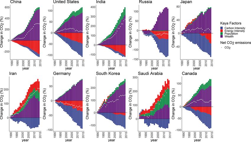
(1990–2015) using a decomposition analysis of the Kaya identity. The decompositions for the top 10 emitting
countries show that, although similarities exist, countries have unique factors driving their patterns of emissions,
suggesting the need for diverse strategies to mitigate carbon emissions to meditate anthropogenic climate change.
The data for this particular version of CDIAC-FF are available at https://doi.org/10.5281/zenodo.4281271 (Gil-
fillan et al., 2020a).
1 Introduction targets and as verification that these reductions are occurring.
The global carbon cycle is directly influenced by FFCO2
Monitoring emissions of carbon dioxide (CO2 ) to the atmo- emissions, and periodic updates through emissions invento-
sphere from fossil fuel combustion, non-energy use of fos- ries provide information concerning the magnitude and ex-
sil fuels, and other industrial processes is necessary due to tent of these impacts (Friedlingstein et al., 2019, 2020). In-
the role of CO2 emissions in driving anthropogenic climate formation from FFCO2 emission inventories reveals whether
change and because of the importance and prospects for re- emissions are increasing or decreasing, which parties are
ducing emissions. Emissions of CO2 impact climate systems, driving these trends, and what fuel types and economic fac-
ecosystems, and human systems. Fossil CO2 (FFCO2 ) emis- tors are contributing to emissions.
sions inventories are important tools as nations, corporations, Current FFCO2 inventories are compiled using data from
and individuals grapple with deciding appropriate reduction the production, consumption, and trade of fossil fuels and
Published by Copernicus Publications.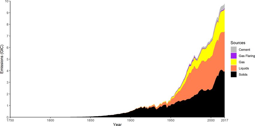
1668                                        D. Gilfillan and G. Marland: CDIAC-FF: global and national fossil CO2 emissions

processes associated with the decomposition of carbonate,          pendent, third-party verification but is difficult due to fluxes
e.g., the production of cement. Data concerning production         of naturally sourced CO2 .
and consumption of fossil fuels are assembled by multi-                The longest, most consistent time series dataset on CO2
ple national and international agencies: the United Nations        emissions has long been the time series of global and national
(UN), the International Energy Agency (IEA), the United            emissions generated by the Carbon Dioxide Information and
States Energy Information Administration (EIA), and BP             Analysis Center (CDIAC) at Oak Ridge National Laboratory
company being prominent (Andres et al., 2012; Hutchins et          (ORNL) (Andres et al., 2012; Marland and Rotty, 1984). The
al., 2017). Depending on the emissions inventory focus, these      CDIAC emissions dataset extends from the beginning of the
fossil fuel data can be used to estimate CO2 emissions by          industrial era (1751) to essentially the present and estimates
fuel type (solids, liquids, and gases) and/or for emissions as-    emissions from fossil fuel oxidation and cement manufac-
sociated with sectors of human activity (energy, transporta-       ture for all countries (Andres et al., 2012; Friedlingstein et
tion, manufacture, etc.). Some inventories may also include        al., 2019, 2020; Le Quéré et al., 2018). The CDIAC annual
emissions from additional industrial processes that emit CO2 ,     inventories began in 1984 when global interest in CO2 emis-
such as cement manufacture, or emissions from the flaring of       sions was limited to the scientific community, although esti-
natural gas.                                                       mates of global emissions had been produced earlier (Keel-
   Emissions of CO2 from fossil fuel consumption are sel-          ing, 1973). Marland and Rotty 1984 laid out the core and de-
dom measured directly, except in recent years at some power        tails of the CDIAC methodology, and these have generally
plants and other very large point sources, (e.g., United States    been unchanged since that publication. The CDIAC emis-
Environmental Protection Agency, 2018). FFCO2 emissions            sions estimates for the years since 1950 are based largely on
are generally estimated from the amount of carbon-based fu-        energy statistics from the UN Statistics Division (United Na-
els that are consumed. Cement manufacture is often included        tions Statistics Division, 2020). The time requirement for the
in CO2 inventories because it is the largest industrial pro-       international data collection and processing is such that the
cess leading to CO2 emissions that does not involve fossil         UN releases this annual database on a 2- to 3-year time lag,
fuel combustion (Conneely et al., 2001). Cement manufac-           which is subsequently reflected in the timeline of the CDIAC
ture emits CO2 into the atmosphere through the process of          FFCO2 emission estimates.
converting calcium carbonate to lime, an essential ingredi-            The CDIAC FFCO2 inventory has a cosmopolitan user
ent of cement. The FFCO2 emissions from fossil fuel com-           base; it is currently integral in the Global Carbon Project’s
bustion used to support cement manufacture are already in-         annual carbon budget (Canadell et al., 2007; Friedlingstein
cluded in CO2 emissions inventories (Andres et al., 2012;          et al., 2019, 2020; Le Quéré et al., 2018), has provided data
Andrew, 2019; Le Quéré et al., 2018). Although other indus-        for the Intergovernmental Panel on Climate Change (IPCC)
trial processes discharge CO2 into the atmosphere, e.g., iron      periodic reports, informs deliberations within the UN, and
and steel production, they are often not currently included        is utilized by the public and the media as a comprehensive
in emissions inventories because of incomplete data and the        resource for trends in CO2 emissions. However, the United
recognition that their quantities are generally less than the      States Department of Energy (USDOE) ceased support for
uncertainty associated with FFCO2 emissions (Andres et al.,        this service at ORNL in 2017. The last release supported by
2012). Natural gas flaring occurs as a byproduct of petroleum      the USDOE included emissions estimates for the year 2014
and natural gas extraction and processing, such as in oil fields   (Boden et al., 2017). The CDIAC CO2 emissions time se-
that are not well connected to natural gas markets, and the re-    ries was restored in 2019 with independent support from Ap-
lated CO2 emissions are included in some global and national       palachian State University. The most recent update (through
inventories.                                                       2017) is the focus of this paper. The historical emissions
   Although the ultimate goal of inventories is record keep-       data from CDIAC at ORNL are stored at the USDOE’s En-
ing of FFCO2 emissions, the foci, boundary conditions, as-         vironmental Systems Science Data Infrastructure for a Vir-
sumptions, and initial data sources make each of the cur-          tual Ecosystem (ESS-DIVE) data repository at the Lawrence
rently existing inventories unique. Inventories can also dif-      Berkeley National Laboratory. CDIAC at ORNL supported
fer on how to deal with fuel used in international transport       a plethora of additional carbon-related research, but this re-
(bunker fuels), which industrial processes are included, and       vival is aimed solely at the important dataset of CO2 emis-
sometimes even which countries are included. However, con-         sions, so the Appalachian State University initiative is iden-
sistency within a dataset is important, and changes to any of      tified hereafter as CDIAC-FF.
these aspects with time or place need to be noted. It is also          Decomposition analysis is an important tool that can be
important to realize that while each of the current inventories    used to characterize temporal drivers of CO2 emissions, ad-
presents estimates of emissions of CO2 for global, regional,       dressing issues such as why certain developed countries are
and/or national totals, the independent verification of emis-      declining in emissions (Le Quéré et al., 2019), assessing the
sions is not presently possible. Estimates are based on survey     socioeconomic aspects of emissions (Pui and Othman, 2019),
data, derived average values, and large quantities of compiled     or identifying drivers of emissions in specific countries using
data. Space-based monitoring may eventually provide inde-          a variety of decomposition techniques (Brizga et al., 2014;

Earth Syst. Sci. Data, 13, 1667–1680, 2021                                         https://doi.org/10.5194/essd-13-1667-2021
D. Gilfillan and G. Marland: CDIAC-FF: global and national fossil CO2 emissions                                            1669

O’Mahony, 2013). The most commonly used approach for              IEA staff experts – and follows the IPCC guidelines for emis-
this kind of analysis with regard to FFCO2 has involved           sions inventories (Andres et al., 2012; Andrew, 2020a; Inter-
the Kaya identity, which relates FFCO2 to four primary fac-       governmental Panel on Climate Change, 2006; OECD/IEA,
tors: population, per capita gross domestic product (GDP)         2020a). The IEA data are for CO2 emissions from the energy
(wealth), energy used per unit of GDP (energy intensity of        sector and do not include emissions from fossil fuel prod-
the economy), and CO2 emitted per unit of energy used (car-       ucts that are used for non-energy applications such as lubri-
bon intensity of the energy system) (Kaya, 1989). The IPCC        cants and solvents and do not include emissions from gas
has used the Kaya identity to support analysis of emissions       flaring or cement manufacture, but they do include emissions
scenarios (Pachauri et al., 2014), although much of their fo-     from bunker fuels in their estimates of global total emissions.
cus on reducing emissions has been on the two elements of         The IEA does include some non-energy uses from iron and
energy consumption and carbon intensity. While the Kaya           steel manufacture and recently provides separate emissions
identity has its limitations, it has regularly been employed      estimates from flaring emissions not within their main CO2
due to the availability of quality data and its clear messages    database (OECD/IEA, 2020b). Recently the IEA has pub-
and general simplicity (O’Mahony, 2013; Pui and Othman,           lished estimates of 2019 global emissions within 2 months
2019).                                                            of the year’s end, based on partial-year data plus some na-
   In this paper we first review the methodology to produce       tional and market data releases (OECD/IEA, 2020c).
the CDIAC-FF emissions estimates (Sect. 2.2) and iden-               The EIA collects their own energy statistics from annual,
tify changes that have been implemented in the transition         national-level reports from countries and uses an approach
from ORNL to Appalachian State University (Boden et al.,          similar to the approach of CDIAC-FF (Andres et al., 2012).
2017; Marland and Rotty, 1984). Two significant changes are       They use internally generated data on the carbon content of
noted: the method of including data on stock changes for cal-     fuels and estimates of the fraction-oxidized coefficients in
culating global totals of CO2 emissions (Sect. 2.2.1) and the     their calculations (Andres et al., 2012; Energy Information
approach for calculating CO2 emissions from the production        Administration, 2020). EIA inventories do include bunker fu-
of cement (Sect. 2.2.4). We also discuss trends in the 2017       els in national totals, along with emissions from gas flaring
time series of CO2 (Sect. 3.1) and compare our estimates to       and adjustment for non-fuel uses but do not include cement
other available global inventories (Sect. 3.2). Further, we de-   manufacture.
compose the Kaya identity for the top 10 emitting countries          EDGAR is produced as a joint effort of the Joint Research
to illustrate the drivers of emissions trends from 1990 to 2015   Centre of the European Commission and the PBL Nether-
(the end date dictated by the availability of necessary sup-      lands Environmental Assessment Agency. EDGAR uses the
porting data) and the challenge that different countries face     energy balance statistics of the IEA in a sectoral approach
in making significant reductions in emissions (Sect. 3.3).        using the IPCC guidelines for emissions estimates and rep-
                                                                  resents the emissions from bunker fuels, gas flaring, carbon-
                                                                  ate decomposition (including cement manufacture), and non-
2     Materials and methods
                                                                  fuel uses using Tier I IPCC methods (Andres et al., 2012;
2.1    Other global datasets of CO2 emissions from fossil
                                                                  Crippa et al., 2018, 2019, 2020). Note that all of the stud-
       fuel combustion
                                                                  ies that estimate emissions from cement production partially
                                                                  rely on cement data from the United States Geological Sur-
There are currently four other prominent, annual, global          vey (van Oss, 2020).
FFCO2 emissions inventories available that are “primary”             The BP Statistical Review of World Energy is the most
emissions databases. This means that, like CDIAC-FF, the          current FFCO2 inventory, with estimates of emissions re-
estimates are derived directly from energy data sources.          ported up to the most recent complete calendar year (BP,
There are also secondary inventories that synthesize their        2020). Their estimates for the 2 most recent years are often
estimates from multiple primary sources (Andrew, 2020a;           used by other inventories to extrapolate emissions values for
Hoesly et al., 2018). These primary datasets are available        the 2 most recent calendar years (Myhre et al., 2009). This al-
from the IEA, EIA, Emissions Database for Global Atmo-            lows the Global Carbon Project, EDGAR, and other FFCO2
spheric Research (EDGAR), and BP Statistical Review of            spatially explicit inventories to report more-current estimates
World Energy. Andres et al. (2012) provide a brief discussion     of global FFCO2 for researchers and the public (Crippa et al.,
of their general characteristics, and recently Andrew (2020a)     2019; Friedlingstein et al., 2019; Oda and Maksyutov, 2011;
has provided a more detailed analysis of the similarities and     Oda et al., 2018). The BP dataset uses IPCC emissions fac-
differences of each of these primary and secondary datasets.      tors but only considers fuels for combustion, with no distinc-
   The IEA estimates emissions for both a reference approach      tion for bunker fuels and no gas flaring or other industrial
(based on fuel type) and a sectoral approach using their own      processes (BP, 2020).
energy questionnaire for members and some additional coun-
tries, data sharing with the UN for many other countries,
national statistical publications, and the best estimates from

https://doi.org/10.5194/essd-13-1667-2021                                        Earth Syst. Sci. Data, 13, 1667–1680, 2021
1670 D. Gilfillan and G. Marland: CDIAC-FF: global and national fossil CO2 emissions
2.2 CDIAC-FF fossil fuel CO2 emissions estimates products, i.e., we estimate that, on a global average, a net
6.7 % of the carbon in liquid fuels, 1 % of gaseous fuels, and
2.2.1 Global fossil fuel CO2 emissions
0.8 % of solids fuels produced in a given year are sequestered
CDIAC-FF uses the UN energy statistics, collected in an an- in long-lived products (Marland and Rotty, 1984). This im-
nual questionnaire to all countries, to estimate CO2 emis- plies that the balance between the production of long-lived
sions (Pachauri et al., 2014). The information contained in products in any year and the oxidation of long-lived products
the UN dataset includes production, imports, exports, and produced in earlier years is such that the total amount of fu-
changes of stock for all fuels used for energy and non-energy els sequestered in long-lived products increases by the above
uses. The UN also includes data on fuels that are used in in- percentages of annual production (Marland and Rotty, 1984).
ternational transport, known as bunker fuels, and for fuels In the update to this time series that first included data
not categorized as fossil fuels, e.g., wood and other biofuels. for 2016, we implemented a change in our computation for
Biofuels are not included in estimating CO2 emissions from the estimation of the global total of FFCO2 emissions. All
fossil fuel combustion. The UN period of record dates from CDIAC datasets prior to the CDIAC-FF dataset with data for
1950 to essentially the present, with a 2- to 3-year time lag 2016 have used only production data, with a global-average
between the initiation of collection and final publication of value for FOi , for the estimation of global total emissions for
each year’s data. This is a dynamic dataset in which changes, solids, liquids, and gases, as well as for emissions from gas
additions, and deletions occur with each annual update of flaring. However, the 2016 UN energy statistics revealed a
the energy statistics, based on reporting from each individual substantial drawdown of fuel stocks already produced and on
country. CDIAC-FF is a reference approach to CO2 emis- hand, especially for the solid fuels, and this inspired a refine-
sions, meaning that we are focused on emissions from differ- ment of the CDIAC-FF calculation. Historically, reporting of
ent types of fuel rather than from different economic sectors. changes in stocks to the UN Statistics Division has been such
We estimate emissions for three fuel types (solids, liquids, that the data could be used for some countries but were in-
gases) as well as for gas that is flared and for cement manu- complete for use on total global stocks. Our assumption, in
facture. CO2 estimates based on fuel type facilitate tracking essence, was that at the global level there was no net change
mass flows among parties and makes possible ancillary esti- in stocks each year.
mates such as flows for C isotopes (Andres et al., 2000). The reporting of stock change transactions in the primary
Some key differences exist between the approach for esti- UN energy data has been increasing with time and is now
mating the global total of fossil fuel emissions and for esti- judged complete enough to use in the global FFCO2 emis-
mating national totals. Fuel production data have tradition- sions estimates – while maintaining consistency with histori-
ally been used by CDIAC for global totals, whereas con- cal estimates. The data show 2 years in which the abundance
sumption data have been the standard for estimating national of reported data on stock change transactions increased no-
totals. The reason for this is the lower uncertainty in pro- tably in richness – 1970 and 1992. By 1992 the data on stock
duction data at the global level; fewer data points are needed changes approach the completeness seen in recent year ac-
to calculate production totals rather than consumption totals. counts – and this is also the point at which the dissolution of
Calculations for CO2 emissions are conceptually simple and the Soviet Union had occurred, the unification of Germany
are the product of three terms: the amount of fuel i produced was complete, and the array of countries in the dataset was
(Pi ), the carbon content of the fuel (Ci ), and the fraction of stabilizing. Thus, inclusion of stock changes is now part of
carbon that is oxidized (FOi ) (Eq. 1; see also Marland and the estimation of global CO2 emissions going back to 1992.
Rotty, 1984). Units for Pi and values used for FOi and the Figure 1 shows the quantitative impact of including changes
Ci for each fuel type are summarized in Table 1. in stocks in the estimation of annual, global-total CO2 emis-
sions. While 2016 was a noteworthy year in which inclu-
CO2 (as C) = Pi FOi Ci (1) sion of changes in stocks resulted in a significant increase in
the global estimate of fossil fuels consumed, there are other
A consequence of using fuel production data to estimate years where this is also a noteworthy effect. A net increase in
global total CO2 emissions is that all non-energy uses of fos- global stocks on hand leads to an overestimate of emissions
sil fuels are included in the global totals, as are bunker fuels. if stock changes are not included in the computation and an
At the national level, however, we also deal with issues of underestimate of emissions when global stocks are decreas-
trade, the portion of fuels used outside of national borders, ing. The average of total global emissions with the change in
and fuels that are not oxidized. National totals need to esti- stocks included (from 1970 to 2017), compared with global
mate the amount of fuel products that go into long-term prod- total emissions from production data alone, is 0.26 % lower.
ucts and specifically exclude fuels used in international trans- This shows that the quantity of stocks in hand has not been
port. A correction factor (part of FOi in Eq. 1) is included in changing substantially from year to year but is, on average,
the global total calculation to account for the effective frac- increasing slowly over time. It is therefore important that the
tion of fuel production that is not oxidized in the year of global emissions time series now includes changes in stocks,
production because of sequestration in long-lived, non-fuel and this is reflected in CDIAC-FF emissions estimates.
Earth Syst. Sci. Data, 13, 1667–1680, 2021 https://doi.org/10.5194/essd-13-1667-2021D. Gilfillan and G. Marland: CDIAC-FF: global and national fossil CO2 emissions 1671
Table 1. Units in primary data source and calculation assumptions for fossil fuel combustion CO2 emissions estimates. TJ: terajoules (1012 J);
t C: metric tons of carbon; tce: metric tons of coal equivalent; Mt C: megatons (metric) of carbon (106 t C).
Emissions Transaction units Fraction oxidized Carbon content Ci
source from UN FOi
Solid fuels Metric tonsa 0.982 0.7374 t C tce−1 (hard coal)
0.768 t C tce−1 (brown coal)
Liquid fuels Metric tons 0.918b 0.855 t C t−1
0.985c
Gas fuels TJ 0.98 13.7 Mt C TJ−1
Gas flaring TJ 1.00 13.45 Mt C TJ−1
a Metric tons are converted to energy units in tons of coal equivalent where 1 tce = 2.937 × 10¹⁰ joules. b The
fraction of oxidized liquid fuels used from global totals. c The fraction of oxidized liquid fuels when non-fuel
uses are subtracted out for national totals.
Figure 1. The change in estimated global total CO2 emissions by including changes in stocks as opposed to just using production data, in
megatons of carbon (Mt C). In 2016, the change in global total emissions (orange) corresponds to a 1.10 % underestimation of emissions if
drawdown of stocks is not included in the calculation of global total emissions. This is mostly attributable to changes in stocks of solid fuels
(purple), where including the change in stock results led to an increase of 3.15 % in emissions from solid fuels. Negative values indicate that
there was an increase in stocks on hand and that CO2 emissions would be overestimated if stock changes were not included. We concluded
that data on changes in stocks were sufficiently comprehensive to be included in calculations of CO2 emissions after 1992.
2.2.2 National fossil fuel CO2 emissions used in for non-energy purposes, 0.8 % and 1 % respectively
(Marland and Rotty, 1984). CO2 emissions from bunker fu-
Fuel consumption data are more informative than fuel pro-
els are thus included in estimates of global total emissions
duction data for scales smaller than global totals because lo-
but not included in the country totals except to designate the
cal specificity is needed to properly allocate emissions. At
country where fuel loading took place. Emissions of CO2
the national level fuel consumption (Eq. 2) is estimated us-
will occur along international shipping lanes, not in the coun-
ing apparent consumption (ACi ) and is substituted for Pi in
try where fuel loading took place. Non-energy (non-fuel)
Eq. (1). Apparent consumption is defined as
uses involve fuel commodities that are used for applications
ACi = Pi + Ii − Ei − Bi − NEi − SCi , (2) that are not directly consumed for energy uses; examples
would be petroleum liquids used to make plastics, lubricants,
where Pi represents production for a given fuel type i, Ii rep- and asphalt or fertilizer production using natural gas (Mar-
resents imports, Ei represents exports, Bi represents bunker land and Rotty, 1984). When the sum of emissions from all
fuel loadings, NEi represents non-energy uses that are un- country totals does not equal the global total, there are three
oxidized, and SCi represents stock changes. NEi values are primary reasons: emissions from bunker fuels are included
explicitly subtracted out for liquids based on the UN en- in the global, but not in national, totals; emissions from fu-
ergy statistics codes, and we use the global assumptions els produced for non-energy uses are estimated based on as-
(Sect. 2.2.1) for the amount of solid and gaseous fuels that are
https://doi.org/10.5194/essd-13-1667-2021 Earth Syst. Sci. Data, 13, 1667–1680, 20211672 D. Gilfillan and G. Marland: CDIAC-FF: global and national fossil CO2 emissions
sumptions in the global total, but at the national level non- series of emissions. To provide estimates of CO2 emissions
energy uses are explicitly subtracted out for particular prod- from cement production that are transparent and consistent
ucts before estimation of CO2 ; and the sum of imports for all over time and space, we rely, when possible, on clinker pro-
countries does not equal the sum of exports globally because duction data that are publicly available and likely to be up-
of statistical errors and incomplete reporting. dated regularly (Case 1). Where data on clinker production
are not available, we rely on data for cement production and
2.2.3 Per capita emissions
best estimates of the clinker-to-cement ratio (Case 2). Emis-
sions of CO2 from cement production, Ecement , are calculated
The CDIAC-FF dataset includes estimates of CO2 emissions as follows (Andrew, 2019).
per capita from 1950 onward. The UN World Population Case 1:
Prospects data are used for global and national level calcu- MCO2 CaO
lations (United Nations Department of Economic and So- Ecement = 1.02 r Mclinker (3)
MCaO clinker
cial Affairs – Population Division, 2020). The projections
Case 2:
are produced annually by the UN population division, and
MCO2 CaO clinker
we use the standard, rather than the probabilistic, projections Ecement = 1.02 r r Mcement (4)
of population. MCaO clinker cement
MCO
Here MCaO2 is the molecular weight ratio of CO2 to CaO,
2.2.4 Global and national emissions from cement CaO is the ratio of CaO in clinker (64.6 %), r clinker is the
rclinker cement
manufacture clinker ratio, Mclinker is the mass of clinker produced, and
The manufacture of cement involves calcining carbonate Mcement is the mass of the cement produced. Since the advent
rock, e.g., limestone, to produce CaO-rich clinker, a primary of widespread national reporting of greenhouse gas emis-
ingredient in cement production. The production of clinker sions to the United Nations Framework Convention on Cli-
through calcination is one of the largest non-fossil-fuel com- mate Change (UNFCCC), many countries have been report-
bustion sources of CO2 emissions. The clinker is then finely ing values for clinker production in their national inventory
ground with gypsum and sometimes other additives to pro- reports. Time series of clinker production back to 1990 are
duce finished cement. Calculations based on cement produc- now available for 31 countries in these national inventory re-
tion were, and still are, facilitated by a global database of ce- ports, and we use these clinker production data to calculate
ment production by country maintained initially by the U.S. emissions in Case 1. We also adopt the Intergovernmental
Bureau of Mines and subsequently by the USGS (van Oss, Panel on Climate Change (2006) addition of 2 % for cement
2020). kiln dust that is not captured in the cement product
to gener-
MCO2 CaO
The biggest change in CDIAC-FF is in the estimates of ate a final emission factor 1.02 MCaO rclinker of 0.52 kg CO2
CO2 emissions from cement manufacture. The CDIAC emis- per kilogram of clinker (0.142 kg C per kilogram of clinker).
sion factor for CO2 from cement manufacture has remained While cement manufacture is the third largest source of an-
constant and time invariant since 1987, with the estimates thropogenic CO2 emissions (after fossil fuel use and land-use
based directly on the chemistry of then-current data on world change), the availability of the data required for estimating
average cement. Since that time, however, the quantity of emissions needs improvement (Andrew, 2019). However, for
additives in blended cements has increased broadly; that is clinker are becoming
many countries and regions estimates of rcement
the fraction of clinker in finished cements has decreased as clinker
increasingly available. The average rcement globally declined
additives such as coal fly ash and blast furnace slag have from 83 % in 1990 to 78 % in 2006 and continued to drop to
increased (Ke et al., 2013; Kim and Worrell, 2002). This 67 % in 2013, with a rebound after 2013 (Andrew, 2019). The
made it clear that the original CDIAC methodology was over- Cement Sustainability Initiative, Getting the Numbers Right,
estimating CO2 from cement manufacture (Andrew, 2018, is a global effort to collect environmental data on the global
2019), especially from China, which now produces over half cement industry. It was begun in 2006 by the World Business
of the world’s cement (van Oss, 2020), and required a re- Council for Sustainable Development, and at the beginning
evaluation of the assumptions for our calculation. of 2019, the work on the effort was transferred to the Global
Since the clinker content of cement has been declining Cement and Concrete Association (GCCA) (Global Cement
since before 1990, and varies with time and place, it follows and Concrete Association, 2020).
that the best practice for calculating CO2 emissions from ce- Large quantities of data, including values for rcement clinker , are
ment manufacture should be based on the amount of clinker now reported by the GCCA, which we use for individual
in finished cements (Andrew, 2018; Intergovernmental Panel countries with no clinker production data in national inven-
On Climate Change, 2006). The availability of good data on tory reports. There is also an extensive literature on CO2
clinker production or the clinker content of cements really emissions from cement manufacture in China. From this pub-
begins in 1990, so we have updated CO2 emissions estimates licly available literature we assembled a consistent time se-
back to 1990 for the recent edition of the CDIAC-FF time clinker for Chinese cement production
ries of the historic rcement
Earth Syst. Sci. Data, 13, 1667–1680, 2021 https://doi.org/10.5194/essd-13-1667-2021D. Gilfillan and G. Marland: CDIAC-FF: global and national fossil CO2 emissions 1673
since 1990 (Cai et al., 2016; Gao et al., 2017; Ke et al., 2012, 2015, the growth rate began increasing again in 2016, with
2013; Kim and Worrell, 2002; Liu et al., 2015; Shen et al., a growth rate of 0.5 % in 2016 and 1.2 % in 2017. Although
2015; Wei and Cen, 2019). The IPCC 2006 inventory guide- all three fuel groups showed an increase from 2016–2017,
lines do not endorse the process of calculating CO2 emis- a 3.1 % increase in natural gas emissions was the primary
sions directly from cement production data, but the dearth driver of the growth in overall global FFCO2 emissions.
of international data on clinker production and trade dictates Emissions from cement manufacture decreased by 1.5 %
clinker to estimate clinker production from ce-
that using a rcement from 2016 to 2017. Since 1990, global emissions have in-
ment data is often the best choice commonly available. creased by 61.8 %, with emissions from solid fuels increas-
ing by 67.2 %, liquid fuels increasing by 37.6 %, natural gas
2.2.5 Decomposition of recent CO2 emissions trends increasing by 90.8 %, and cement manufacture increasing by
184 %. Emissions from solid fuels contribute the most to the
The Kaya identity, first described by Yoichi Kaya (Kaya, 2017 global total (3.94 Gt C, or 40.2 %), followed by emis-
1989), is a way for us to evaluate factors that drive past and sions from liquid fuels (3.43 Gt C, or 35 %), emissions from
future trends in emissions. The Kaya identity states that fossil gases (1.96 Gt C, or 20 %), emissions from cement manufac-
CO2 emissions (C) can be expressed as the product of four ture (384 Mt C, or 3.9 %), and emissions from the flaring of
terms: natural gas (76 Mt C or 0.7 %). The uncertainties associated
GDP E C with each of these global estimates are described by Andres
C≡P × × × = Cp × CW × CEI × CCI , (5) et al. (2014).
P GDP E
The top 10 emitting countries now collectively emit ap-
where P is population, GDP is gross domestic product (pur- proximately 65 % of the world’s total emissions. The top 10
chasing power parity, PPP; current international dollars), and emitters represent countries from North America, Europe,
E is primary energy consumption. Data are available from and Asia. These 10 countries’ emissions and 2016–2017
the World Bank on each of these variables (World Bank, growth rates as well as population changes and per capita
2019). The four factors provide simple representations of emissions are summarized in Table 2. China has been the
population (Cp ) and the complex factors of wealth (CW ), the global leader in emissions since 2005 with emissions that
structure and efficiency of the economy (CEI ), and the carbon have grown by 301 % since 1990. The total Chinese CO2
intensity of the energy system (CCI ). We discuss the four fac- emissions declined from 2014–2016 but saw a 1.7 % increase
tors in these simple terms. We decompose emissions using in total CO2 emissions in 2017. Because of the implications
a logarithmic mean Divisia index (LMDI) approach (Ang, of being such a large emitter of CO2 , accurate accounting
2005; Le Quéré et al., 2019), and we report relative changes is important for Chinese emissions; however, there is uncer-
over time in CO2 emissions due to each of the four Kaya tainty associated with Chinese data due in part to uncertainty
factors. For the change in C (1C) between 2 given years, in in coal quality (Han et al., 2020).
this case year t2 and the reference year t1 , the identity can be The country with the largest relative growth in emissions
decomposed as follows: from 2016 to 2017 in the top 10 emitters was Iran, increas-
ing by 11.84 %. This is reportedly driven by a 74 % increase
1C = 1Cp + 1CW + 1CEI + 1CCI , (6) in emissions from the flaring of natural gas (8.9 Mt C), fol-
lowed by a 12.1 % increase in emissions from liquid fuel
where combustion (6.6 Mt C) and a 4.9 % increase in the emission
C t2 − C t1 Cxt2 from natural gas combustion (5.1 Mt C). India’s emissions
1Cx = ln ; (7) now (2017) are double its 2005 value as it continues to transi-
ln (C t2 ) − ln (C t1 ) Cxt1
tion as an emergent economy, and the total CO2 emissions in-
i.e., 1Cx is the change in CO2 emissions (estimated from creased by 5.0 % from 2016. Russian emissions are the fourth
CDIAC-FF country totals) over the interval t1 (reference largest in the world and grew at a rate similar to that of In-
year) to t2 which is attributable to Kaya factor x (Ang, 2005). dia in 2017. Two countries among the top 10 emitters show
We decomposed CO2 emissions attributable to each of the decreases in CO2 emissions from 2016 to 2017 – the United
factors annually from 1990 to 2015; data were not available States’ and Germany. The United States and Germany’s de-
to 2017 for each of the World Bank datasets. creases are attributed to decreases in solid fuel consumption.
Zambia (37.7 %), Mongolia (35.3 %), Saint Helena
(33.3 %), Mauritania (31.65 %), and Brunei (26.3 %) demon-
3 Results
strated the largest growth rates from 2016 to 2017. The coun-
tries that experienced the largest losses in emissions were
3.1 Recent trends in global and national emissions
North Korea (21.0 %), the British Virgin Islands (20.3 %),
The global total for CO2 emissions from fossil fuel oxida- United Arab Emirates (18.1 %), Ghana (16.9 %), and Eswa-
tion and cement manufacture in 2017 was 9.79 Gt C (Fig. 2). tini (16.4 %). These negative values are mostly due to eco-
After a period of slowing annual growth between 2010 and
https://doi.org/10.5194/essd-13-1667-2021 Earth Syst. Sci. Data, 13, 1667–1680, 20211674 D. Gilfillan and G. Marland: CDIAC-FF: global and national fossil CO2 emissions
Figure 2. Total global CO2 emissions from fossil fuel combustion and cement manufacture from 1950 to 2017, partitioned into fuel type,
cement production, and gas flaring. Emissions are in gigatons of carbon.
Table 2. Top 10 CO2 -emitting countries with total CO2 emissions in 2017, population in 2017, the changes in population and emissions
from 2016 to 2017, and the 2017 per capita emissions.
Rank Nation Total CO2 Population Emissions change Population change Per capita CO2
emissions (millions) 2016–2017 (%) 2016–2017 (%) emissions
(Mt C) (t C per person)
1 China 2646 1421 1.67 0.49 1.86
2 United States of America 1351 325 −0.70 0.64 4.11
3 India 671 1339 5.00 1.07 0.50
4 Russia 494 145 4.99 3.39
5 Japan 314 128 0.32 −0.23 2.46
6 Islamic Republic of Iran 198 81 11.84 1.40 2.46
7 Germany 196 83 −0.83 0.57 2.37
8 Republic of Korea 169 51 0.49 0.22 3.31
9 Saudi Arabia 156 33 2.74 2.02 4.72
10 Canada 156 37 4.32 0.96 4.25
nomic downturns/instability, civil unrest, and potential sta- Comparisons are not simple, but we briefly summarize the
tistical anomalies, particularly for very small countries. alternate data sources and the differences that they convey
(Sect. 2.1). Figure 2 compares the final estimates of global
total emissions for 4 years (1990, 2000, 2016, 2017) and a
3.2 Comparing the different global fossil fuel CO2 sampling of data for six diverse countries that include the
emissions inventories three largest emitting countries.
Although systematic comparison of the alternate datasets
As noted above, there are currently five primary sources for
has been undertaken (Andrew, 2020a; Ciais et al., 2010;
global estimates of CO2 emissions: CDIAC-FF, IEA, EIA,
Hutchins et al., 2017; Macknick, 2009; Marland et al., 1999,
EDGAR, and BP. These emissions inventories have been pre-
2007) the system boundaries and assumptions used in the cal-
pared by different parties with different objectives, different
culations make this comparison difficult. Andres et al. (2012)
emphases, different system boundaries, and different results.
attempted to put them on common ground and found that the
Some, for example, include emissions from cement manufac-
global CO2 emissions agreed to within 3 % of the mean (An-
ture while some do not, but we compare the gross reported
dres et al., 2012), and this estimate is similar to more recent
total of CO2 emissions as included in the respective reports.
Earth Syst. Sci. Data, 13, 1667–1680, 2021 https://doi.org/10.5194/essd-13-1667-2021D. Gilfillan and G. Marland: CDIAC-FF: global and national fossil CO2 emissions 1675
comparative analyses (Andrew, 2020a). Our goal here is to
demonstrate a general accord that includes the reinvigorated
CDIAC-FF.
Absolute percent differences range from 0.12 % to 19.6 %
depending on the country and are less than 10 % for the
global totals for all 4 years (Fig. 3). At the country level, all of
the higher estimates of CO2 emissions (> 10 %), compared
to CDIAC-FF, come from the EDGAR and EIA datasets,
while the lower estimates of CO2 (≤ −10 %) come from the
IEA, EIA, and BP datasets. Since EDGAR includes other
carbonates, this explains some of the reasoning for the higher
estimates of CO2 emissions in countries where carbonate de-
composition is larger than others, and since IEA does not
include cement production or flaring, this explains some the
lower estimates of CO2 emissions.
The larger underestimates are generally from the coun-
tries of Ecuador, Morocco, and India, while the larger over-
estimates, compared to CDIAC-FF, come from China and
France. We suggest that the differences are generally not in-
dicative of accuracy but rather an indication of the different
system boundaries and a measure of the uncertainty; for an
extended discussion of possible errors from India, see An-
drew (2020b). Overall, we estimate that global total emis-
sions have increased by 61.8 % since 1990 and from 2016 to
2017 grew by 1.2 %. The other datasets report growth from
1990 to 2016 as 56.0 % to 62.2 % and show a similar growth
rate from 2016 to 2017 (1.0 % to 1.4 %).
Since we have recently updated the procedure for the esti-
mation of CO2 from cement manufacture, it is prudent to also
compare the new cement estimates with previous estimates
from the ORNL CDIAC, for which the last inventory year
is 2014, and a comprehensive global CO2 inventory (An-
drew, 2019). Table 3 outlines the total CO2 emissions from Figure 3. Comparison of four other global emissions datasets with
cement manufacture for the globe and the top five cement- CDIAC-FF for 1990, 2000, 2016, and 2017. Specific emissions
producing countries in each of these datasets. For global to- datasets are cited in Sect. 2.1. The 0 % centerline represents exact
tals, ORNL CDIAC estimates grow from 16 % higher than agreement with the CDIAC-FF value. Six countries and the global
these new CDIAC-FF estimates in 1990 to 48 % higher in totals were selected to illustrate the variability between datasets and
2014, indicating the overestimation of CO2 emissions be- countries. Shapes represent each of the years, and colors represent
cause of using the time- and location-invariant emission fac- each of the datasets. Box plots are used to show the general distri-
tor for cement. CDIAC-FF’s global total of CO2 emissions bution of the percent difference, with the dark line in the box rep-
from cement manufacture is within 5 % of Andrew (2019). resenting the median percent difference, the box representing the
range of the 25th and 75th percentiles, and the whiskers represent-
China is a particular country to focus on in this comparison
ing the overall range of the data. This demonstrates that with few
due to its role as the leading producer of cement since 1982. exceptions the estimations are all within 10 % of CDIAC-FF esti-
ORNL CDIAC’s estimates of CO2 from cement manufac- mates for the selected countries and years.
ture in China are 34 % higher than the CDIAC-FF estimates
in 1990, but this grows to 68 % higher in 2014. Much like
the global comparisons, Andrew (2019) and CDIAC-FF are results are presented as percentage contributions of the four
within 5 % of each other. Kaya-based factors (population, wealth, energy intensity of
the economy, and carbon intensity of the energy system) to
3.3 Decomposition of recent trends in CO2 emissions CO2 emissions changes based on the reference year estimates
(Fig. 4). For sake of discussion, we will describe positive
To gain insight into what is driving changes in CO2 emissions changes attributable to a specific Kaya factor as drivers of
at the country level, decomposition analysis was performed CO2 emissions, while negative change will be described as
on the top 10 emitting countries for the period 1990–2015, offsets of CO2 emissions.
or 1992–2015 for Russia and 1991–2015 for Germany. The
https://doi.org/10.5194/essd-13-1667-2021 Earth Syst. Sci. Data, 13, 1667–1680, 20211676 D. Gilfillan and G. Marland: CDIAC-FF: global and national fossil CO2 emissions Figure 4. Log mean Divisia index (LMDI) decomposition of Kaya factors for the top 10 CO2 -emitting countries. The Kaya factors are outlined in Eq. (3), and the decomposition calculation is outlined in Eqs. (4) and (5). Changes are relative to the reference year 1990 for all countries, except Germany (reference year 1991) and Russia (reference year 1992). Positive values indicate drivers of increases in emissions, while negative values indicate offsetting factors. Net CO2 emissions relative to the reference year are presented by gray dots. The countries are shown in order, from top left to bottom right, of their total CO2 emissions for the year 2017. With the exception of the impacts of the dissolution of the only nation in the top 10 emitting countries in which popu- Soviet Union on Russia, increasing wealth (per capita GDP) lation growth is the dominant driving force (132 % increase, is a driving force on increasing emissions in each of the top relative to 1990 values); decreasing carbon intensity of the 10 emitting countries. This is especially evident in China, energy system only provides modest offsets (33 % decrease) where increasing wealth has contributed to a 561 % increase to increasing CO2 emissions. in CO2 emissions from 1990–2015. China’s growth in wealth The remaining top 10 emitters (United States, Russia, is partially offset by decreases in energy intensity (250 % de- Japan, Germany, and Canada) are all Annex-I countries with crease in 2015, relative to 1990). Other countries that see this obligations to regularly report emissions to the UNFCCC. pattern of increasing wealth substantially driving emissions The countries are characterized by increasing wealth having are India (312 % increase from 1990–2015) and South Korea the largest-magnitude influence on CO2 emissions, but this is (243 % increase from 1990–2015). These are emergent, de- offset by decreases in carbon intensity followed by decreases veloping economies representing some of the fastest growing in energy intensity. Population growth only contributes min- economies in the world since 1990. The dominant offsetting imally to the trends in emissions in each of these countries, factors for these countries are decreasing energy intensity for and in some cases (Russia) decreasing population is a small India (116 % decrease) and decreasing carbon intensity for offsetting factor for CO2 emissions. South Korea (106 % decrease). Saudi Arabia and Iran, the top emitting countries from the 4 Data availability Middle East, exhibit unique characteristics of the Kaya fac- tors in which energy intensity is a driving force in increas- The exact version of the CDIAC-FF time series of ing emissions in addition to population growth and increas- CO2 emissions from fossil fuel combustion and ce- ing wealth. In Iran, 116 % of the growth in emissions from ment manufacture that is described in this publication 1990 to 2015 can be attributed to increasing wealth, 79 % to is located here: https://doi.org/10.5281/zenodo.4281271 increasing energy intensity, and 61 % to population growth. (Gilfillan et al., 2020a). The historic record of These are modestly offset by decreases in carbon intensity CDIAC products from ORNL is archived here: of the energy system (50 % decrease). Saudi Arabia is the https://doi.org/10.3334/CDIAC/00001_V2017 (Boden Earth Syst. Sci. Data, 13, 1667–1680, 2021 https://doi.org/10.5194/essd-13-1667-2021
D. Gilfillan and G. Marland: CDIAC-FF: global and national fossil CO2 emissions                                                1677

Table 3. Comparison of estimates of CO2 emissions from cement       countries in estimating the bulk of FFCO2 emissions from
manufacture for the globe and the top five cement-producing coun-   oxidation and cement production. In continuing the CDIAC-
tries. Data are from the most recent CDIAC-FF update, the last      FF dataset at Appalachian State, we provide long-term conti-
ORNL CDIAC inventory update, and an independent inventory pro-      nuity while continuing to provide updates and refinements as
duced by Andrew (2019).                                             knowledge and available data permit. Improving availability
                                                                    of data on stock changes of global fuels and data on produc-
    Country/world   Dataset        1990    2000   2010    2014
                                                                    tion of clinker has permitted improved estimates in the 2017
    Global total    ORNL CDIAC      157     226     446    568      CDIAC-FF dataset.
    (Mt C)          CDIAC-FF        135     188     323    385         In addition to evaluating changes in FFCO2 emissions over
                    Andrew 2019     137     195     341    401      time, we illustrate what is driving recent changes for the top
    China (Mt C)    ORNL CDIAC      28.6   81.1     248    339      10 emitting countries. To evaluate the possibilities for lim-
                    CDIAC-FF        21.4     61     159    202      iting emissions in the future, it is useful to understand what
                    Andrew 2019       23   66.6     174    212      is driving changes currently. Population growth, increasing
    India (Mt C)    ORNL CDIAC       6.6   12.9    29.9    37.4     wealth, changes in the energy intensity of the economy, and
                    CDIAC-FF         6.1     12    24.2    25.2     changes in the carbon intensity of energy all force emissions
                    Andrew 2019      6.1   12.5    24.9    29.5     in trajectories unique to each country’s social capital and en-
    USA (Mt C)      ORNL CDIAC       9.7   12.2     9.1    11.3     ergy resources. Among the top 10 emitting countries, major
                    CDIAC-FF         8.9   11.3     8.6    10.7     differences occur in the balance of forces driving changes
                    Andrew 2019      9.1   11.3     8.6    10.8     in CO2 emissions. For example, emissions from Germany,
                                                                    with a net decline in emissions from 1991 onwards, is being
    Turkey (Mt C)   ORNL CDIAC       3.3    4.9     8.5     9.7
                    CDIAC-FF         2.9    4.1     7.9       9
                                                                    driven primarily by changes in energy intensity while emis-
                    Andrew 2019      2.8    4.1       8     9.1     sions growth in Saudi Arabia is being driven more by popula-
                                                                    tion growth. The Kaya decomposition approach employed is
    Vietnam         ORNL CDIAC       0.3    1.8     7.6     8.2
                                                                    simple but provides a framework for more extended analysis
    (Mt C)          CDIAC-FF         0.3    1.7     6.3     6.7
                    Andrew 2019      0.3    1.5     5.8     6.3
                                                                    of the complex factors driving changes in emissions. Our de-
                                                                    compositions suggest that while much of the previous analy-
                                                                    sis on a Kaya framework has focused on energy and carbon
                                                                    intensity, there is a need to characterize the more difficult as-
et al., 2017). Future and previous updates from CDIAC-FF            pects of carbon mitigation: growth in population and wealth.
produced at Appalachian State University will be in-                   The future and equitable confrontation of climate change
cluded at https://doi.org/10.15485/1712447 (Gilfillan et al.,       mitigation will rely on appropriate accounting of CO2 emis-
2020b). The most recent inventory year will also be located         sions across countries and across time. The top 10 emit-
within the Appalachian Energy Center’s website (https:              ting countries each have a unique combination of drivers of
//energy.appstate.edu/research/work-areas/cdiac-appstate,           changing emissions and the need for diverse strategies to mit-
last access: 7 December 2020). This includes .csv files for         igate carbon emissions. National and global inventories will
global and national totals as well as a ranking of each coun-       provide evidence of whether planned emissions reductions
try with regard to total emissions and per capita emissions         are taking place.
for a given year.

5     Conclusions                                                   Author contributions. DG      conceived the content of the
                                                                    manuscript, performed all data analysis and management, and
FFCO2 emissions inventories are integral tools to evaluate          contributed to manuscript development. GM conceived the initial
sources of CO2 emissions, document trends concerning fuel           CDIAC-FF methodology, provided edits and suggestions, collected
                                                                    data on clinker production and clinker ratios, and contributed to
and/or sectoral-based values, and verify that intended reduc-
                                                                    manuscript development.
tions are indeed occurring. While each of five available “pri-
mary” global emissions inventories is unique in approach,
focus, system boundaries, time interval covered, and appli-         Competing interests. The authors declare that they have no con-
cation, the small differences in overall emissions estimates        flict of interest.
suggest the accuracy and integrity of the different products
and statistical approaches. Differences do not reflect the de-
gree of accuracy since independent verification is not cur-         Acknowledgements. The authors would like to thank the helpful
rently available at the global and national scales, especially      suggestions of Robbie Andrew and the one anonymous reviewer for
for CO2 emissions for which there are both natural and an-          improving the quality and content of this paper.
thropogenic sources. CDIAC-FF provides a long-term time
series of FFCO2 emissions that is consistent over time and

https://doi.org/10.5194/essd-13-1667-2021                                                Earth Syst. Sci. Data, 13, 1667–1680, 2021
1678 D. Gilfillan and G. Marland: CDIAC-FF: global and national fossil CO2 emissions
Review statement. This paper was edited by David Carlson and pean carbon balance. Part 1: fossil fuel emissions, Glob. Change
reviewed by Robbie Andrew and one anonymous referee. Biol., 16, 1395–1408, 2010.
Conneely, D., Gibbs, M. J., and Soyka, P.: CO2 emissions from
industry, in: Good Practice Guidance and Uncertainty Manage-
References ment in National Greenhouse Gas Inventories, Intergovernmental
Panel on Climate Change, available at: https://www.ipcc-nggip.
Andres, R., Marland, G., Boden, T., and Bischof, S.: Carbon dioxide iges.or.jp/public/gp/english/3_Industry.pdf (last access: 7 De-
emissions from fossil fuel consumption and cement manufacture, cember 2020), 2001.
1751–1991, and an estimate of their isotopic composition and Crippa, M., Guizzardi, D., Muntean, M., Schaaf, E., Dentener,
latitudinal distribution, in: The Carbon Cycle, edited by: Wigley, F., van Aardenne, J. A., Monni, S., Doering, U., Olivier,
T. and Schimel, D., 53–62, Cambridge University Press, New J. G. J., Pagliari, V., and Janssens-Maenhout, G.: Grid-
York, USA, 2000. ded emissions of air pollutants for the period 1970–2012
Andres, R. J., Boden, T. A., Bréon, F.-M., Ciais, P., Davis, S., within EDGAR v4.3.2, Earth Syst. Sci. Data, 10, 1987–2013,
Erickson, D., Gregg, J. S., Jacobson, A., Marland, G., Miller, https://doi.org/10.5194/essd-10-1987-2018, 2018.
J., Oda, T., Olivier, J. G. J., Raupach, M. R., Rayner, P., Crippa, M., Guizzardi, D., Muntean, M., Schaaf, E., Lo Vullo, E.,
and Treanton, K.: A synthesis of carbon dioxide emissions Solazzo, E., Monforti-Ferrario, F., Olivier, J., and Vignati, E.:
from fossil-fuel combustion, Biogeosciences, 9, 1845–1871, EDGAR v5.0 Greenhouse Gas Emissions, available at: https://
https://doi.org/10.5194/bg-9-1845-2012, 2012. edgar.jrc.ec.europa.eu/dataset_ghg50data (last access: 31 August
Andres, R. J., Boden, T. A., and Higdon, D.: A new eval- 2020), 2019.
uation of the uncertainty associated with CDIAC estimates Crippa, M., Guizzardi, D., Muntean, M., Schaaf, E., Solazzo, E.,
of fossil fuel carbon dioxide emission, Tellus B, 66, 23616, Monforti-Ferrario, F., Olivier, J. G. J., and Vignati, E.: Fossil
https://doi.org/10.3402/tellusb.v66.23616, 2014. CO2 emissions of all world countries – 2020 Report, EUR 30358
Andrew, R. M.: Global CO2 emissions from cement production, EN, Publications Office of the European Union, Luxembourg,
Earth Syst. Sci. Data, 10, 195–217, https://doi.org/10.5194/essd- JRC121460, https://doi.org/10.2760/143674, 2020.
10-195-2018, 2018. Energy Information Administration: International energy statis-
Andrew, R. M.: Global CO2 emissions from cement pro- tics, available at: https://www.eia.gov/international/data/world/
duction, 1928–2018, Earth Syst. Sci. Data, 11, 1675–1710, other-statistics/emissions-by-fuel, last access: 31 August 2020.
https://doi.org/10.5194/essd-11-1675-2019, 2019. Friedlingstein, P., Jones, M. W., O’Sullivan, M., Andrew, R. M.,
Andrew, R. M.: A comparison of estimates of global carbon dioxide Hauck, J., Peters, G. P., Peters, W., Pongratz, J., Sitch, S., Le
emissions from fossil carbon sources, Earth Syst. Sci. Data, 12, Quéré, C., Bakker, D. C. E., Canadell, J. G., Ciais, P., Jack-
1437–1465, https://doi.org/10.5194/essd-12-1437-2020, 2020a. son, R. B., Anthoni, P., Barbero, L., Bastos, A., Bastrikov, V.,
Andrew, R. M.: Timely estimates of India’s annual and monthly Becker, M., Bopp, L., Buitenhuis, E., Chandra, N., Chevallier,
fossil CO2 emissions, Earth Syst. Sci. Data, 12, 2411–2421, F., Chini, L. P., Currie, K. I., Feely, R. A., Gehlen, M., Gilfillan,
https://doi.org/10.5194/essd-12-2411-2020, 2020b. D., Gkritzalis, T., Goll, D. S., Gruber, N., Gutekunst, S., Har-
Ang, B. W.: The LMDI approach to decomposition anal- ris, I., Haverd, V., Houghton, R. A., Hurtt, G., Ilyina, T., Jain,
ysis: a practical guide, Energ. Policy, 33, 867–871, A. K., Joetzjer, E., Kaplan, J. O., Kato, E., Klein Goldewijk, K.,
https://doi.org/10.1016/j.enpol.2003.10.010, 2005. Korsbakken, J. I., Landschützer, P., Lauvset, S. K., Lefèvre, N.,
Boden, T., Marland, G., and Andres, R. J.: Global, Regional, and Lenton, A., Lienert, S., Lombardozzi, D., Marland, G., McGuire,
National Fossil-Fuel CO2 Emissions (1751–2014) (V. 2017), P. C., Melton, J. R., Metzl, N., Munro, D. R., Nabel, J. E. M. S.,
Carbon Dioxide Information Analysis Center (CDIAC), Oak Nakaoka, S.-I., Neill, C., Omar, A. M., Ono, T., Peregon, A.,
Ridge National Laboratory (ORNL), Oak Ridge, TN, USA, Pierrot, D., Poulter, B., Rehder, G., Resplandy, L., Robertson, E.,
https://doi.org/10.3334/CDIAC/00001_V2017, 2017. Rödenbeck, C., Séférian, R., Schwinger, J., Smith, N., Tans, P. P.,
BP: Statistical review of world energy, available at: Tian, H., Tilbrook, B., Tubiello, F. N., van der Werf, G. R., Wilt-
https://www.bp.com/en/global/corporate/energy-economics/ shire, A. J., and Zaehle, S.: Global Carbon Budget 2019, Earth
statistical-review-of-world-energy.html, last access: 31 August Syst. Sci. Data, 11, 1783–1838, https://doi.org/10.5194/essd-11-
2020. 1783-2019, 2019.
Brizga, J., Feng, K., and Hubacek, K.: Drivers of greenhouse gas Friedlingstein, P., O’Sullivan, M., Jones, M. W., Andrew, R. M.,
emissions in the Baltic States: A structural decomposition analy- Hauck, J., Olsen, A., Peters, G. P., Peters, W., Pongratz, J., Sitch,
sis, Ecol. Econ., 98, 22–28, 2014. S., Le Quéré, C., Canadell, J. G., Ciais, P., Jackson, R. B., Alin,
Cai, B., Wang, J., He, J., and Geng, Y.: Evaluating CO2 emission S., Aragão, L. E. O. C., Arneth, A., Arora, V., Bates, N. R.,
performance in China’s cement industry: an enterprise perspec- Becker, M., Benoit-Cattin, A., Bittig, H. C., Bopp, L., Bultan,
tive, Appl. Energy, 166, 191–200, 2016. S., Chandra, N., Chevallier, F., Chini, L. P., Evans, W., Florentie,
Canadell, J. G., Le Quéré, C., Raupach, M. R., Field, C. B., Buiten- L., Forster, P. M., Gasser, T., Gehlen, M., Gilfillan, D., Gkritza-
huis, E. T., Ciais, P., Conway, T. J., Gillett, N. P., Houghton, R. lis, T., Gregor, L., Gruber, N., Harris, I., Hartung, K., Haverd, V.,
A., and Marland, G.: Contributions to accelerating atmospheric Houghton, R. A., Ilyina, T., Jain, A. K., Joetzjer, E., Kadono, K.,
CO2 growth from economic activity, carbon intensity, and effi- Kato, E., Kitidis, V., Korsbakken, J. I., Landschützer, P., Lefèvre,
ciency of natural sinks, P. Natl. Acad. Sci. USA, 104, 18866– N., Lenton, A., Lienert, S., Liu, Z., Lombardozzi, D., Marland,
18870, 2007. G., Metzl, N., Munro, D. R., Nabel, J. E. M. S., Nakaoka, S.-I.,
Ciais, P., Paris, J. D., Marland, G., Peylin, P., Piao, S. L., Levin, I., Niwa, Y., O’Brien, K., Ono, T., Palmer, P. I., Pierrot, D., Poul-
Pregger, T., Scholz, Y., Friedrich, R., and Rivier, L.: The Euro-
Earth Syst. Sci. Data, 13, 1667–1680, 2021 https://doi.org/10.5194/essd-13-1667-2021You can also read