RainBench: Towards Global Precipitation Forecasting from Satellite Imagery
←
→
Page content transcription
If your browser does not render page correctly, please read the page content below
RainBench: Towards Global Precipitation Forecasting from Satellite Imagery
                                           Christian Schroeder de Witt*1 , Catherine Tong*1 , Valentina Zantedeschi2 , Daniele De Martini1 ,
                                                   Freddie Kalaitzis1 , Matthew Chantry1 , Duncan Watson-Parris1 , Piotr Biliński3
                                                                                    1
                                                                                      University of Oxford (*: Equal contribution)
                                                  2
                                                      Inria, Lille - Nord Europe research centre and University College London, Centre for Artificial Intelligence
                                                                                                3
                                                                                                  University of Warsaw
arXiv:2012.09670v1 [cs.LG] 17 Dec 2020

                                                                     Abstract                                 However, while there have been attempts in forecasting pre-
                                                                                                              cipitation with neural networks, they have mostly been frag-
                                           Extreme precipitation events, such as violent rainfall and hail
                                                                                                              mented across different local regions, which hinders a sys-
                                           storms, routinely ravage economies and livelihoods around
                                           the developing world. Climate change further aggravates this       tematic comparison into their performance.
                                           issue (Gupta et al. 2020). Data-driven deep learning ap-              In this work, we introduce RainBench, a multi-modal
                                           proaches could widen the access to accurate multi-day fore-        dataset to support data-driven forecasting of global pre-
                                           casts, to mitigate against such events. However, there is          cipitation from satellite imagery. We curate three types of
                                           currently no benchmark dataset dedicated to the study of           datasets: simulated satellite data (SimSat), numerical re-
                                           global precipitation forecasts. In this paper, we introduce        analysis data (ERA5), and global precipitation estimates
                                           RainBench, a new multi-modal benchmark dataset for data-           (IMERG). The use of satellite images to forecast precipi-
                                           driven precipitation forecasting. It includes simulated satel-     tation globally would circumvent the need to collect ground
                                           lite data, a selection of relevant meteorological data from the
                                           ERA5 reanalysis product, and IMERG precipitation data. We
                                                                                                              station data, and hence they are key to our vision for widen-
                                           also release PyRain, a library to process large precipitation      ing the access to multi-day precipitation forecasts. Reanal-
                                           datasets efficiently. We present an extensive analysis of our      ysis data provide estimates of complete atmospheric state,
                                           novel dataset and establish baseline results for two bench-        and IMERG provides rigorous estimates of global precipita-
                                           mark medium-range precipitation forecasting tasks. Finally,        tion. Access to these data opens up opportunities to develop
                                           we discuss existing data-driven weather forecasting method-        more timely and potentially physics-informed forecast mod-
                                           ologies and suggest future research avenues.                       els, which so far could not have been studied systematically.
                                                                                                                 Most related to our work, Rasp et al. (2020) have devel-
                                                                 Introduction                                 oped WeatherBench, a benchmark environment for global
                                                                                                              data-driven medium-range weather forecasting. This dataset
                                         Extreme precipitation events, such as violent rain and hail          forms an excellent first step in weather forecasting. How-
                                         storms, can devastate crop fields and disrupt harvests (Vo-          ever, some important features of WeatherBench limit its use
                                         gel et al. 2019; Li et al. 2019). These events can be locally        for end-to-end precipitation forecasts. WeatherBench does
                                         forecasted with sophisticated numerical weather models that          not include any observational raw data (e.g. satellite data)
                                         rely on extensive ground and satellite observations. How-            and only contains ERA5 reanalysis data, which have limited
                                         ever, such approaches require access to compute and data             resolution of extreme precipitation events. Further, Weather-
                                         resources that developing countries in need - particularly in        Bench does not include a fast dataloading pipeline to train
                                         South America and West Africa - cannot afford (Le Coz and            ML models, which we found to be a significant bottle-
                                         van de Giesen 2020; Gubler et al. 2020). The lack of ad-             neck in our model development and testing process. This
                                         vance planning for precipitation events impedes socioeco-            gap prompted us to also release PyRain, a data processing
                                         nomic development and ultimately affects the livelihoods of          and experimentation framework with fast and configurable
                                         millions around the world. Given the increase in global pre-         multi-modal dataloaders.
                                         cipitation and extreme precipitation events driven by climate
                                                                                                                 To summarise our contributions: (a) We introduce the
                                         change (Gupta et al. 2020), the need for accurate precipita-
                                                                                                              multi-modal RainBench dataset which supports data-driven
                                         tion forecasts is ever more pressing.
                                                                                                              investigations for global precipitation forecasting from satel-
                                            Data-driven machine learning approaches circumvent
                                                                                                              lite imagery; (b) we release PyRain, which allows re-
                                         the dependence on traditional resource-intensive numerical
                                                                                                              searchers to run Deep Learning (DL) experiments on Rain-
                                         models, which typically take several hours to run (Sønderby
                                                                                                              Bench efficiently, reducing time and hardware costs and thus
                                         et al. 2020), incurring a significant time lag. In contrast, deep
                                                                                                              lowering the barrier to entry into this field; (c) we intro-
                                         learning models deployed on dedicated high-throughput
                                                                                                              duce two benchmark precipitation forecasting tasks on Rain-
                                         hardware can produce inferences in a matter of seconds.
                                                                                                              Bench and their baseline results, and present experiments
                                         Copyright © 2021, Association for the Advancement of Artificial      studying class-balancing schemes. Finally, we discuss the
                                         Intelligence (www.aaai.org). All rights reserved.                    challenges in the field and outline several fruitful avenues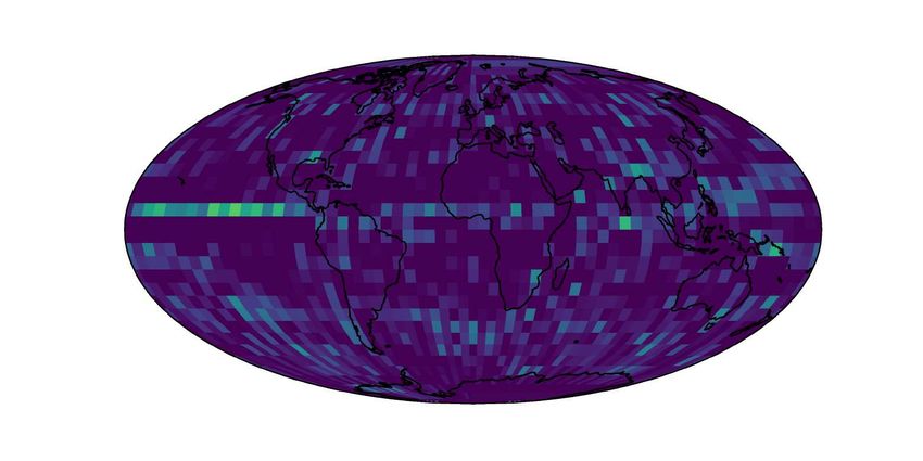
for future research.                                               provides no route to producing an end-to-end forecasting
                                                                   system.
                       Related Work
Weather forecasting systems have not fundamentally                                         RainBench
changed since they were first operationalised nearly 50 years
ago. Current state-of-the-art operational weather forecasting      In this section, we introduce RainBench, which consists
systems rely on numerical models that forward the physi-           of data derived from three publicly-available sources: (1)
cal atmospheric state in time based on a system of physi-          European Centre for Medium-Range Weather Forecasts
cal equations and parameterised subgrid processes (Bauer,          (ECMWF) simulated satellite data (SimSat), (2) the ERA5
Thorpe, and Brunet 2015). While global simulations typi-           reanalysis product, and (3) Integrated Multi-satellitE Re-
cally run at grid sizes of 10 km, regional models can reach        trievals (IMERG) global precipitation estimates.
1.5 km (Franch et al. 2020) . Even in the latter case, skilled     SimSat We use simulated satellite data in place of real
forecast lengths are usually limited to a maximum of 10            satellite imagery to minimise data processing requirements
days, with a conjectured hard limit of 14 to 15 days (Zhang        and to simplify the prediction task. SimSat data are model-
et al. 2019). Nowcasting, i.e. high-resolution weather fore-       simulated satellite data generated from ECMWF’s high-
casting only a few hours in advance, is currently limited by       resolution weather-forecasting model using the RTTOV ra-
the several hours that numerical forecasting models take to        diative transfer model (Saunders et al. 2018). SimSat emu-
run (Sønderby et al. 2020).                                        lates three spectral channels from the Meteosat-10 SEVIRI
   Given the huge amounts of data currently available from         satellite (Aminou 2002). SimSat provides information about
both numerical models and observations, new opportunities          global cloud cover and moisture features and has a native
exist to train data-driven models to produce these forecasts.      spatial resolution of about 0.1° – i.e. about 10 km – at three-
The current boom in Machine Learning (ML) has inspired             hourly intervals. The product is available from April 2016
several other groups to approach the problem of weather            to present (with a lag time of 24 h). Using simulated satel-
forecasting. Early work by Xingjian et al. have invested us-       lite data provides an intermediate step to using real satel-
ing convolutional recurrent neural networks for precipita-         lite observations as the images are a global nadir view of
tion nowcasting. More recently, Sønderby et al. from Google        Earth, avoiding issues of instrument error and large num-
proposed a “(weather) model free” approach, MetNet, which          bers of missing values. Here we aggregate the data to 0.25°
seeks to forecast precipitation in continental USA using geo-      – about 30 km – to be consistent with the ERA5 dataset.
stationary satellite images and radar measurements as in-
puts. This approach performs well up to 7-8 hours, but in-         ERA5 We use ERA5 as it is an accurate and commonly
evitably runs into a forecast horizon limit as information         used reanalysis product familiar to the climate science com-
from global or surrounding geographic areas is not incor-          munity (Rasp et al. 2020). ERA5 reanalysis data provides
porated into the system. This time window has value though         hourly estimates of a variety of atmospheric, land and
it would not enable substantial disaster preparedness.             oceanic variables, such as specific humidity, temperature
   The prediction of extreme precipitation (and other ex-          and geopotential height at different pressure levels (Hers-
treme weather events) has a long history with traditional          bach et al. 2020). Estimates cover the full globe at a spatial
forecasting systems (Lalaurette 2003). More recent devel-          resolution of 0.25° and are available from 1979 to present,
opments in ensemble weather forecasting systems surround           with a lag time of five days.
the introduction of novel forecasting indices (Zsótér 2006,
EFI) and post-processing (Grönquist et al. 2020). There has       IMERG IMERG is a global half-hourly precipitation es-
also been other deep-learning based precipitation forecast-        timation product provided by NASA (Huffman et al. 2019).
ing models as motivated by the monsoon prediction prob-            We use the Final Run product which primarily uses satellite
lem, for example, Saha, Mitra, and Nanjundiah (2017) and           data from multiple polar-orbiting and geo-stationary satel-
Saha et al. (2020) use a stacked autoencoder to identify           lites. This estimate is then corrected using data from re-
climatic predictors and an ensemble regression tree model,         analysis products (MERRA2, ERA5) and rain-gauge data.
while Praveen et al. (2020) use kriging and multi-layer per-       IMERG is produced at a spatial resolution of 0.1° – about
ceptrons to predict monsoon rainfall from ERA5 data.               10 km – and is available from June 2000 to present, with a
   WeatherBench (Rasp et al. 2020) is a benchmark dataset          lag time of about three to four months.
for data-driven global weather forecasting, derived from data         To facilitate efficient experimentation, all data is con-
in the ERA5 archive. Its release has prompted a number             verted from thier original resolutions to 5.625° resolutions
of follow-up works to employ deep learning techniques for          using bilinear interpolation.
weather forecasting, although the variables considered have           RainBench provides precipitation values from two
only been restricted to the forecasts of relatively static vari-   sources, ERA5 and IMERG, as both are widely used and
ables, such as 500 hPa geopotential and 850 hPa temper-            considered to be high-quality precipitation datasets. The
ature (Weyn, Durran, and Caruana 2019, 2020; Rasp and              ERA5 precipitation is accumulated precipitation over the
Thuerey 2020; Bihlo 2020; Arcomano et al. 2020). Unlike            last hour and is calculated as an averaged quantity over a
RainBench which incorporates the element of observational          grid-box. We aggregated IMERG precipitation into hourly
input data from (simulated) satellites, WeatherBench’s data        accumulated precipitation and should be considered as a
comes solely from the ERA5 reanalysis archive, and thus            point estimate of the precipitation.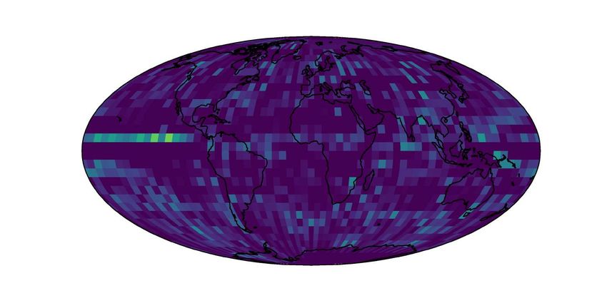
Figure 1 shows the distribution of precipitation for the                                   Table 1: Number of data samples loaded per second using
 years 2000-2017 with both ERA5 and IMERG. IMERG is                                            PyRain versus a conventional NetCDF framework. Typical
 generally regarded as a more trust-worthy dataset for pre-                                    configurations assumed and performed on a NVIDIA DGX1
 cipitation due to the direct inclusion of precipitation obser-                                server with 64 CPUs.
 vations in the data assimilation process and the higher spa-
 tial resolution used to produce the dataset, which also result                                                         NetCDF         PyRain       Speedup
 in seen difference in data distributions. IMERG has signifi-
                                                                                                       16 workers          40           2410         60.3×
 cantly larger rainfall tails than ERA5, and these tails rapidly
                                                                                                       64 workers          70           1930         27.6×
 vanish with decreasing dataset resolution. The underestima-
 tion of extreme precipitation events in ERA5 is clearly visi-
 ble.
                       100                                                                     aloader. We find empirically that PyRain’s memmap dat-
                                                                              ERA:tp 1.40625
                      10   2                                                  ERA:tp 5.625     aloader offers significant speedups over other solutions, sat-
probability density

                                                                              IMERG 0.25       urating even SSD I/O with few process workers when used
                      10   4                                                  IMERG 1.40625
                                                                              IMERG 5.625      with PyTorch’s (Paszke et al. 2019) inbuilt dataloader.
                      10   6
                                                                                                  Note that explicitly storing each training sample is not
                      10   8
                                                                                               only slow and inflexible for research settings, but it also
                      10   10
                                                                                               requires twenty to fifty times more storage and as a result
                                0   25   50    75      100     125      150    175      200    comes at a higher cost than constructing samples on-the-fly.
                                              precipitation [mm/hour]                          Thus, other options such as writing samples in TFRecord
                                                                                               format (Weyn, Durran, and Caruana 2019; Abadi et al. 2016)
 Figure 1: Precipitation histogram from 2000-2017 with                                         would only be sensible for highly distributed training in pro-
 ERA5 and IMERG at different resolutions. Vertical lines de-                                   duction settings.
 lineate convection rainfall types: slight (0–2 mm h−1 ), mod-                                    PyRain’s dataloader is easily configurable and supports
 erate (2–10 mm h−1 ), heavy (10–50 mm h−1 ), and violent                                      both complex multimodal item compositions, as well as pe-
 (over 50 mm h−1 ) (MetOffice 2012).                                                           riodic (Sønderby et al. 2020) and sequential (Weyn, Durran,
                                                                                               and Caruana 2020) train-test set partitionings. Apart from its
                                                                                               data-loading pipeline, PyRain also supplies flexible raw-data
                                                PyRain                                         conversion tools, a convenient interface for data-analysis
 To support efficient data-handling and experimentation on                                     tasks, various data-normalisation methods and a number of
 Rainbench, we release PyRain, an out-of-the-box experi-                                       ready-built training settings based on PyTorch Lightning8 .
 mentation framework.                                                                          While being optimised for use with RainBench, PyRain is
    PyRain1 introduces an efficient dataloading pipeline for                                   also compatible with WeatherBench.
 complex sample access patterns that scales to the terabytes
 of spatial timeseries data typically encountered in the cli-                                                         Evaluation Tasks
 mate and weather domain. Previously identified as a decisive
 bottleneck by the Pangeo community2 , PyRain overcomes                                        We define two benchmark tasks on RainBench for precipi-
 existing dataloading performance limitations through an ef-                                   tation forecasting, with the ground truth precipitation values
 ficient use of NumPy memmap arrays3 in conjunction with                                       taken from either ERA5 or IMERG.
 optimised software-side access patterns.                                                         For each benchmark task, we consider three different in-
    In contrast to storage formats requiring read system calls,                                put data settings: SimSat, reanalysis data (ERA5), or both.
 including HDF54 , Zarr5 or xarray6 , memory-mapped files                                      From the ERA5 dataset, we select a subset of variables as in-
 use the mmap system call to map physical disk space directly                                  put to the forecast model based on our data analysis results;
 to virtual process memory, enabling the use of lazy OS de-                                    the inputs are geopotential (z), temperature (t), humidity
 mand paging and circumventing the kernel buffer. While less                                   (q), cloud liquid water content (clwc), cloud ice water con-
 beneficial for chunked or sequential reads and spatial slicing,                               tent (ciwc), each sampled at 300 hPa, 500 hPa and 850 hPa
 memmaps can efficiently handle the fragmented random ac-                                      geopotential heights; to these we add the surface pressure
 cess inherent to the randomized sliding-window access pat-                                    and the 2-meter temperature (t2m), as well as static vari-
 terns along the primary axis as required in model training.                                   ables that describe the location and surface of the Earth, i.e.
    In Table 1, we compare PyRain’s memmap data read-                                          latitude, longitude, land-sea mask, orography and soil type.
 ing capcity against a NetCDF+Dask 7 (Rocklin 2015) dat-                                       From the SimSat dataset, the inputs are cloud-brightness
                                                                                               temperature (clbt) taken at three wavelengths. We normalize
                      1
                        https://github.com/frontierdevelopmentlab/pyrain                       each variable with its global mean and standard deviation.
                      2
                        https://pangeo.io/index.html (2021)                                       Since data from each source are available at different
                      3
                        https://docs.python.org/3/library/mmap.html (2021)                     times, we use the data subset from April 2016 to train all
                      4
                        https://portal.hdfgroup.org/display/HDF5/HDF5(2021)                    models for the benchmark tasks, unless specified otherwise.
                      5
                        https://zarr.readthedocs.io/en/stable/ (2021)                          We use data from 2018 and 2019 as validation and test sets
                      6
                        http://xarray.pydata.org/en/stable/ (2021)
                      7                                                                           8
                        https://www.unidata.ucar.edu/software/netcdf/ (2021)                          https://pytorch-lightning.readthedocs.io/en/latest/ (2021)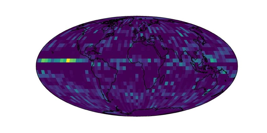
lon                                                 1.00
                                                                        lat
                                                                      lsm                                                  0.75
                                                                       oro
                                                                        slt                                                0.50
                                                                          z
                                                                          t                                                0.25
                                                                          q
                                                                        sp                                                 0.00
Figure 2: Model setup for the benchmark forecasting tasks.          clwc
                                                                    ciwc                                                     0.25
                                                                     t2m
respectively. To make sure no overlap exists between train-        clbt:0                                                    0.50
                                                                   clbt:1
ing and evaluation data, the first evaluated date is 6 January     clbt:2
2019 while the last training date is 31 December 2017.                                                                       0.75
                                                                         tp
   We perform experiments with a neural network based on           imerg                                                     1.00
Convolutional LSTMs, which have been shown to be effec-

                                                                                  oro

                                                                              imerg
                                                                                  lon
                                                                                   lat

                                                                                     q
                                                                                 lsm

                                                                                   slt
                                                                                     z
                                                                                     t

                                                                                   sp
                                                                               clwc
                                                                               ciwc
                                                                                t2m
                                                                              clbt:0
                                                                              clbt:1
                                                                              clbt:2
                                                                                    tp
tive for regional precipitation nowcasting (Xingjian et al.
2015). We structure our forecasting task based on MetNet’s
configurations (Sønderby et al. 2020), where a single model       Figure 3: Spearman’s correlation of RainBench variables
is trained conditioned on time and is capable of forecasting      from April 2016 to December 2019 in latitude band
at different lead times.                                          [−60◦ , 60◦ ] at pressure levels 300 hPa (about 10 km) (up-
   The network’s input is composed of a time series {xt },        per triangle) and 850 hPa (1.5 km) (lower triangle). Leg-
where each xt is the set of standardized features at time t,      end: lon: longitude, lat: latitude, lsm: land-sea mask, oro:
sampled in regular intervals ∆t from t = −T to t = 0; the         orography (topographic relief of mountains), lst: soil type,
output is a precipitation forecast y at lead time t = τ ≤         z: geopotential height, t: temperature, q: specific humidity,
τL . In addition to the aforementioned atmospheric features,      sp: surface pressure, clwc: cloud liquid water content, ciwc:
static features (e.g. latitude) along with three time-dependant   cloud ice water content, t2m: temperature at 2m, clbt:i:
features (hour, day, month) are repeated per timestep. The        ith SimSat channel, tp: ERA5 total precipitation, imerg:
input vector is then concatenated with a lead-time one-hot        IMERG precipitation. All correlations in this plot are sta-
vector xτ . In our experiments, we adopt T = 12 h, ∆t = 3         tistically significant (p < 0.05).
h and forecasts at 24-hour intervals up to τL = 120 h. We
note that we do not include precipitation as an input tempo-
ral feature. An overview of our setup is shown in Figure 2.       non-linear, monotonic relationship between variables, while
   We approach the tasks as a regression problem. Following       Pearson’s considers only linear correlations. This allows
(Rasp et al. 2020), we use the mean latitude-weighted Root-       to capture relationships between variables such as between
Mean-Square Error (RMSE) as loss and evaluation metric.           temperature and absolute latitude. Comparing correlations at
We compare the results to persistence and climatology base-       altitude pressure levels 300 hPa (about 10 km) and 850 hPa
lines. For persistence, precipitation values at t = 0 are used    (1.5 km), we can see that they are almost identical, save
as prediction at t = τ . We compute climatology and weekly        for a few exceptions: Specific humidity, q, and geopotential
climatology baselines from the full training dataset (since       height, z, correlate strongly at 300 hPa but not at 850 hPa,
1979 for ERA5 and since 2000 for IMERG), where local              cloud ice water content, ciwc, generally correlates more
climatologies are computed as a single mean over all times        strongly at higher altitude (and cloud liquid water content,
and per week respectively (Rasp et al. 2020).                     clwc, vice versa). A careful examination of the underlying
                                                                  physical dependencies results in the realisation that all of
                          Results                                 these asymmetries stem mostly from latitudinal correlations
In this section, we first present our data analysis of Rain-      or effects related to cloud formation, e.g. ice and liquid form
Bench. We then describe models’ performance on the bench-         in clouds at different temperatures/altitudes.
mark precipitation forecasting tasks, which highlights the           As we are particularly interested in variables that have
difficulty in forecasting precipitation values on IMERG. Fi-      predictive skill on precipitation, we note that all SimSat
nally, we present an experiment on same-timestep precipita-       spectral channels moderately anti-correlate with both ERA5
tion estimation to investigate class balancing issues.            and IMERG precipitation estimates. Interestingly, SimSat
                                                                  signals correlate much more strongly with specific humid-
Data Analysis                                                     ity and cloud ice water content at higher altitude, which
To analyse the dependencies between all RainBench vari-           might be a consequence of spectral penetration depth. ERA5
ables, we calculate pairwise Spearman’s rank correlation in-      state variables that correlate the most with either precipita-
dices over latitude band from −60 to 60° and date range           tion estimates are specific humidity and temperature. Cloud
from April 2016 to December 2019 (see Figure 3). In con-          ice water content correlates moderately strongly with pre-
trast to Pearson’s correlation coefficient, Spearman’s cor-       cipitation estimates at high altitude, but not at all at lower
relation coefficient is significant if there is a, potentially    altitudes (where ice water content tends to be much lower).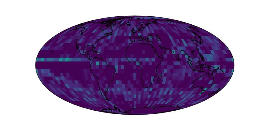
Table 2: Precipitation forecasts evaluated with Latitude-            ture the general precipitation distribution across the globe,
weighted RMSE (mm). All rows except where otherwise                  but there is various degrees of blurriness in the outputs. As
stated show models trained with data from 2016 onwards.              we shall discuss later in the paper, considering probabilistic
                                                                     forecasts would be a promising solution to blurriness, which
              (a) Predicting Precipitation from ERA                  might have arisen as the mean predicted outcome.
                                                                        We also see the importance in using a large training
 Inputs                        1-day       3-day       5-day
                                                                     dataset, since extending the considered training instances to
 Persistence                  0.6249    0.6460    0.6492             the full ERA5 dataset outperforms the baselines further in
 Climatology                      0.4492 (1979-2017)                 the 1-day forecasting regime (shown in the last rows).
 Climatology (weekly)             0.4447 (1979-2017)                    Table 2b shows the forecast results when predicting
 SimSat                       0.4610      0.4678       0.4691        IMERG precipitation. As before, the neural model’s fore-
 ERA                          0.4562      0.4655       0.4677        casting skill based on both SimSat and ERA input outper-
 SimSat + ERA                 0.4557      0.4655       0.4675        forms the other input settings. The higher observed RMSEs
                                                                     suggest that this is a considerably more difficult task, which
 ERA (1979-2017)              0.4485      0.4670       0.4699        we believe to be closely tied to IMERG featuring more ex-
                                                                     treme precipitation events (Figure 1). In the next section, we
            (b) Predicting Precipitation from IMERG                  investigate this issue further by considering a same-timestep
                                                                     precipitation estimation task.
 Inputs                        1-day       3-day       5-day            A key limitation in our current experimental setup is that
 Persistence                  1.1321    1.1497    1.1518             it requires all of ERA5, IMERG and SimSat channels to be
 Climatology                      0.7696 (2000-2017)                 available at each time step, limiting the range of our train-
 Climatology (weekly)             0.7687 (2000-2017)                 ing data to April 2016 and onward. Nevertheless, our neural
                                                                     models significantly outperform persistence baselines. The
 SimSat                       0.8166      0.8201       0.8198        fact that local climatology trained over longer time periods
 ERA                          0.8182      0.8224       0.8215        significantly outperforms our network model baselines sug-
 SimSat + ERA                 0.8134      0.8185       0.8185        gests the development of alternative modelling setups that
 ERA (2000-2017)              0.8085      0.8194       0.8214        can make use of the full available datasets from each source.

                                                                     Same-Timestep Precipitation Estimation
Further, a number of time-varying ERA5 state variables cor-          We now describe a set of experiments for same-timestep pre-
relate more strongly with IMERG precipitation than ERA5              cipitation estimation on IMERG. This analysis is done in-
precipitation, as do SimSat signals. Conversely, a number            dependently from the precipitation forecasting benchmark
of constant variables, such as land-sea mask, orography and          tasks, in order to provide an in-depth understanding of the
soil type are significantly anti-correlated with ERA5 precip-        challenges in modelling extreme precipitation events.
itation, but not at all correlated with IMERG. Overall, we              We use a gradient boosting decision tree learning algo-
find that all variables that are significantly correlated or anti-   rithm (Ke et al. 2017, LightGBM) in order to estimate same-
correlated with both ERA5 tp and IMERG are also corre-               timestep IMERG precipitation directly from ERA5 and Sim-
lated or anti-correlated with SimSat clbt:0-2, suggesting that       Sat. Our training set consists of 1 million randomly sam-
precipitation prediction from simulated satellite data alone         pled grid points/pixels within the time interval April 2016
may be feasible.                                                     to December 2019. We compare the (not latitude-adjusted)
                                                                     RMSE for two pixel sampling variants: A) unbalanced sam-
Precipitation Forecasting                                            pling, meaning grid points are chosen randomly from the
                                                                     raw data distribution and B) balanced sampling, in which
Table 2 compares the neural model forecasts in different             we bin IMERG precipitation into the four classes defined in
data settings when predicting precipitation from ERA5 and            Figure 1 and sample grid points such that we end up with an
IMERG. Using the ERA5 precipitation as target, Table 2a              equal amount of pixels per bin.
shows that training from SimSat alone gives the worst results           In Table 3, we find that taking a balanced sampling ap-
across the data settings. This confirms the difficulty in pre-       proach reduces the per-class validation RMSE of moderate,
cipitation forecast from satellite data alone, which does not        heavy and violent precipitation. This balanced sampling ap-
contain as much information about the atmospheric state as           proach also has detrimental effects on the mean forecast-
sophisticated reanalysis data such as ERA5. Importantly, the         ing performance but not the macro-mean performance, as
complementary benefits of utilizing data from both sources           the ‘slight’ class dominates the dataset and is misclassified
is already visible despite our simple concatenation setup, as        more often. However, balancing the training set does result
training from both SimSat and ERA5 achieves the best re-             in a lower macro RMSE.
sults across all lead times (when holding the number of train-          Designing an appropriate class-balanced sampling may
ing instances constant).                                             play a crucial role toward improving predictions of extreme
   Figure 4 shows example forecasts from one random in-              precipitation events. It is not quite clear how a per-pixel sam-
put sequence across the different data settings for predicting       pling scheme may be translated into a global output context
ERA5 precipitation. We observe that the forecasts can cap-           approach such as in MetNet (Sønderby et al. 2020) where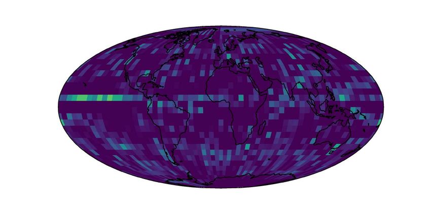
1-day                   2-day                3-day                 4-day                  5-day

      Truth

     Simsat

       ERA

     Simsat
     & ERA

                                Figure 4: ERA5 Precipitation forecasts on one random sample.

Table 3: Comparing RMSE Results with and without a                  in which a model might rarely predict extreme values. De-
class-balanced training dataset. The modelling task is same-        signing an appropriate class sampling strategy (e.g. inverse
timestep estimation of IMERG precipitation.                         frequency sampling) can mitigate this imbalance, as shown
                                                                    in our same-timestep prediction experiments. Further, we
                    L       M    H      V     Mean Macro            believe that a mixture of pixelwise-weighting and balanced
                                                                    sampling could be a potential solution.
 Unbalanced
 ERA          0.20 4.08 16.2 63.1              0.65    20.9         Probabilistic forecasts. The current machine learning
 SimSat       0.20 4.38 16.8 54.1              0.65    18.9         setup produces deterministic predictions, which may lead
 SimSat + ERA 0.20 4.03 16.5 53.0              0.65    18.4         to an averaging of possible futures into a single blurry
 Balanced                                                           prediction. This limitation may be overcome with proba-
                                                                    bilistic modelling, which may take different forms. For in-
 ERA          1.05 2.75 12.4 58.0              1.40    18.6         stance, Sønderby et al. made use of a cross-entropy loss
 SimSat       1.17 3.10 13.3 50.1              1.26    16.9         over a categorical distribution to handle probabilistic fore-
 SimSat + ERA 1.30 3.15 11.8 44.3              1.38    15.1         casts. Stochastic video prediction techniques (Babaeizadeh
                                                                    et al. 2018) and conditional generative adversarial learning
                                                                    (Mirza and Osindero 2014) have also been shown to pro-
each individual pixel’s input distribution should be kept bal-      duce realistic predictions in other fields. Other relevant tech-
anced, while training as many pixels per input data sample          niques that predict distribution parameters are Variational
as possible for efficiency. A possible way of navigating this       Auto-Encoders (Kingma and Welling 2014) and normaliz-
challenge would be to sample greedily, i.e. based on the cur-       ing flows (Rezende and Mohamed 2016).
rently most imbalanced pixel and combine this with learning
rate adjustments for other pixels trained on the same frame         Data normalisation. Feature scaling is a common data-
based on how imbalanced these pixels are at that timestep.          processing step for training machine learning models and
                                                                    well-understood to be advantageous (Bhanja and Das 2019).
                        Discussion                                  Our current approach normalizes each variable using its
                                                                    global mean and standard deviation; This disregards any
We outline the key challenges in global precipitation fore-         local spatial differences, which is important for modelling
casting, our proposed solutions, we also discuss promising          local weather patterns (Weyn, Durran, and Caruana 2019).
research avenues that can build on our work.                        Previous work suggested that patch-wise normalisation may
                                                                    be appropriate (Grönquist et al. 2020, Local Area-wise Stan-
Challenges                                                          dardization (LAS)). We suggest studying a refinement to
From our experiments, we identified a number of challenges          LAS, which adjusts the kernel size with latitude such that
inherent to data-driven extreme precipitation forecasting.          the spatial normalisation context remains constant (Latitude-
                                                                    Adjusted LAS) per-channel image-size normalisation.
Class imbalance Extreme precipitation events, by their
nature, rarely occur (see Figure 1). In the context of super-       Data topology. Lastly, the spherical input and output data
vised learning, this manifests as a class imbalance problem,        topology of global forecasting contexts poses interesting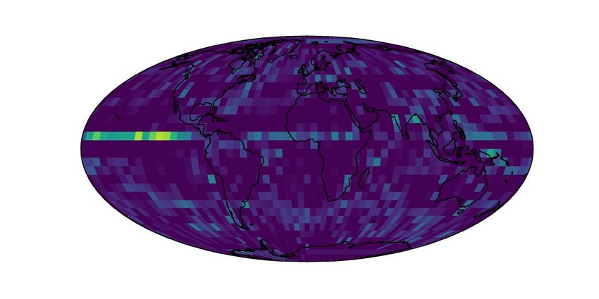
questions to neural network architecture. While a multi-           satellite data becomes available after ca. 4 hours. We pos-
tude of approaches to handle spherical input topologies have       tulate that this lag could be further reduced if, instead of
been suggested, see (Llorens Jover 2020) for an overview, it       high-dimensional observational data, forecasting agencies
seems yet unclear which approach works best. Our dataset           were exchanging their locally processed low-dimensional
might constitute a valuable benchmark for such research.           embeddings derived from local encoder networks. Embed-
                                                                   dings could then be feed into a late fusion network architec-
Future research avenues                                            ture similar to Rudner et al. (2019, Multi3 Net).
Apart from overcoming the challenges outlined above, we
have identified a variety of opportunities for further research.

                                                                   Multi-time-step loss function. Numerical forecasting
Physics-informed multi-task learning. Apart from us-               systems forward the physical state in time by following an
ing reanalysis data for model training, we do not currently        iterative setting, where the output of the previous step is fed
exploit the fact that many aspects of weather forecasting are      as input to the next step. As the update rules are identical for
well-understood from a physical perspective. One way of            each step, it in principle suffices for neural networks to learn
informing model training of physical constraints would be          a single such update step and apply it multiple times during
to train precipitation forecasting concurrently with predic-       inference depending on the prediction lead time, thus reduc-
tion of physical state variables, including temperature and        ing the number of trainable weights and potentially increase
specific humidity, in a multi-task setting, e.g. through using     generalisation performance. To avoid instability issues in-
separate decoder heads for different variables (similarly to       herent to iterative approaches (Rasp et al. 2020), model roll-
Caruana (1997)). This approach promises to combine the ad-         outs can be trained end-to-end (McGibbon and Bretherton
vantages of data-driven learning with low-level feature regu-      2019; Brenowitz and Bretherton 2018). Weyn, Durran, and
larisation through a physics-informed inductive bias. Multi-       Caruana (2020) pioneer this approach but limit themselves
task learning can also be regarded as a form of data aug-          to just two time steps. To overcome device memory con-
mentation (Shorten and Khoshgoftaar 2019), promising to            straints in such a setting and to scale to a large number
further increase forecasting performance using real or sim-        of time steps tollouts, iteration layers could be chosen to
ulated satellite data without requiring access to reanalysis       be reversible (Gomez et al. 2017) such that activations can
data at inference time.                                            be computed on-the-fly during backpropagation and do not
                                                                   need to be stored in device memory.
Increasing spatial resolution. Data at higher spatial res-
olution tends to capture heavy and extreme precipitation
events better but poses a number of challenges. Large sam-                                 Conclusion
ple batch sizes may lead to network activation storage that
exceeds GPU global memory capacity even for distributed            We presented RainBench, a novel benchmark suite for data-
training. Apart from exploring TPU or nvlink-based solu-           driven extreme precipitation forecasting, and PyRain, an as-
tions, another way would be to switch to mixed-precision or        sociated rapid experimentation framework with a fast dat-
half-precision or employ techniques that trade-off memory          aloader. Both RainBench and PyRain are open source and
for compute such as gradient checkpointing (Pinckaers, van         well-documented. We furthermore present neural baselines
Ginneken, and Litjens 2019). PyRain’s dataloader efficiently       for multi-day precipitation forecasting from both reanalysis
maximises total disk throughput, which may itself become a         and simulated satellite data. Despite our simple approach,
bottleneck at very high resolutions. Storing all or part of the    we find that our neural baselines beat climatology and per-
training data memmaps on one or several high-speed local           sistence baselines for up to 5 day forecasts. In addition, we
SSDs may increase disk throughput a few-fold. Apart from           use a gradient boosting decision tree algorithm to study the
memory and disk throughput, there is also a lack of suitably       impact of precipitation class balancing on regression in a
highly resolved historical climate data for pre-training (Rasp     precipitation estimation setting and present various forms of
et al. 2020). One possible way of overcoming this would be         data exploration, including a correlation study.
to integrate high-resolution local forecasting model or sen-
sor data into the training process (Franch et al. 2020), an-          In the near future, we will augment RainBench with real
other exciting approach spearheaded in computational fluid         satellite data. We plan on also including historical climate
dynamics (Jabarullah Khan and Elsheikh 2019) is to em-             data for pre-training. Concurrently, we will explore various
ploy a multi-fidelity approach, where hierarchical variance-       directions for future research, as discussed above. In partic-
reduction techniques are employed to enable training to be         ular, we believe increasing the spatial resolution of our input
performed at lower-resolution data as often as possible, thus      data is crucial to closing the gap to operational forecasting
minimising the need for training on high-resolution data.          models. Ultimately, we hope that our benchmark and frame-
                                                                   work will lower the barrier of entry for the global research
                                                                   community such that our work contributes to rapid progress
Reducing IMERG Early Run lag time. While the final                 in data-driven weather prediction, democratisation of access
IMERG product becomes available at a time lag of ca. 3-            to adequate weather forecasts and, ultimately, help protect
4 months, a preliminary, Early Run, product based on raw           and improve livelihoods in a warming world.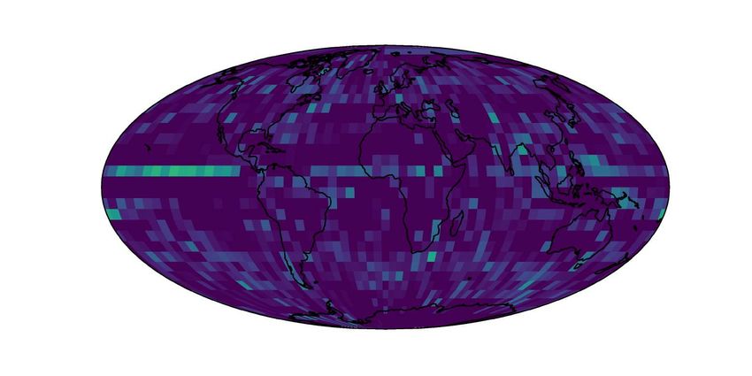
Acknowledgements                                Gomez, A. N.; Ren, M.; Urtasun, R.; and Grosse, R. B.
This research was conducted at the Frontier Development           2017. The Reversible Residual Network: Backpropagation
Lab (FDL), Europe. The authors gratefully acknowledge             Without Storing Activations. arXiv:1707.04585 [cs] ArXiv:
support from the European Space Agency ESRIN Phi                  1707.04585.
Lab, Trillium Technologies, NVIDIA Corporation, Google            Grönquist, P.; Yao, C.; Ben-Nun, T.; Dryden, N.; Dueben,
Cloud, and SCAN. The authors are thankful to Peter                P.; Li, S.; and Hoefler, T. 2020. Deep Learning for Post-
Dueben, Stephan Rasp, Julien Brajard and Bertrand Le Saux         Processing Ensemble Weather Forecasts .
for useful suggestions.
                                                                  Gubler, S.; Sedlmeier, K.; Bhend, J.; Avalos, G.; Coelho, C.;
                        References                                Escajadillo, Y.; Jacques-Coper, M.; Martinez, R.; Schwierz,
                                                                  C.; de Skansi, M.; et al. 2020. Assessment of ECMWF
Abadi, M.; Agarwal, A.; Barham, P.; Brevdo, E.; Chen, Z.;         SEAS5 seasonal forecast performance over South America.
Citro, C.; Corrado, G. S.; Davis, A.; Dean, J.; Devin, M.;        Weather and Forecasting 35(2): 561–584.
Ghemawat, S.; Goodfellow, I.; Harp, A.; Irving, G.; Isard,
M.; Jia, Y.; Jozefowicz, R.; Kaiser, L.; Kudlur, M.; Lev-         Gupta, A. K.; Yadav, D.; Gupta, P.; Ranjan, S.; Gupta, V.;
enberg, J.; Mane, D.; Monga, R.; Moore, S.; Murray, D.;           and Badhai, S. 2020. Effects of climate change on Agricul-
Olah, C.; Schuster, M.; Shlens, J.; Steiner, B.; Sutskever, I.;   ture. Food and Agriculture Spectrum Journal 1(3).
Talwar, K.; Tucker, P.; Vanhoucke, V.; Vasudevan, V.; Vie-        Hersbach, H.; Bell, B.; Berrisford, P.; Hirahara, S.; Horányi,
gas, F.; Vinyals, O.; Warden, P.; Wattenberg, M.; Wicke,          A.; Muñoz-Sabater, J.; Nicolas, J.; Peubey, C.; Radu, R.;
M.; Yu, Y.; and Zheng, X. 2016. TensorFlow: Large-Scale           Schepers, D.; et al. 2020. The ERA5 global reanaly-
Machine Learning on Heterogeneous Distributed Systems.            sis. Quarterly Journal of the Royal Meteorological Society
arXiv:1603.04467 [cs] .                                           146(730): 1999–2049.
Aminou, D. 2002. MSG’s SEVIRI instrument. ESA                     Huffman, G.; Stocker, E.; Bolvin, D.; Nelkin, E.; and Tan,
Bulletin(0376-4265) (111): 15–17.                                 J. 2019. GPM IMERG Final Precipitation L3 Half Hourly
Arcomano, T.; Szunyogh, I.; Pathak, J.; Wikner, A.; Hunt,         0.1 degree x 0.1 degree V06. Technical report. doi:10.5067/
B. R.; and Ott, E. 2020. A Machine Learning-Based Global          GPM/IMERG/3B-HH/06.
Atmospheric Forecast Model. Geophysical Research Letters          Jabarullah Khan, N. K.; and Elsheikh, A. H. 2019. A Ma-
47(9): e2020GL087776.                                             chine Learning Based Hybrid Multi-Fidelity Multi-Level
Babaeizadeh, M.; Finn, C.; Erhan, D.; Campbell, R. H.;            Monte Carlo Method for Uncertainty Quantification. Fron-
and Levine, S. 2018. Stochastic Variational Video Predic-         tiers in Environmental Science 7. ISSN 2296-665X. Pub-
tion. arXiv:1710.11252 [cs] URL http://arxiv.org/abs/1710.        lisher: Frontiers.
11252. ArXiv: 1710.11252.                                         Ke, G.; Meng, Q.; Finley, T.; Wang, T.; Chen, W.; Ma, W.;
Bauer, P.; Thorpe, A.; and Brunet, G. 2015. The quiet rev-        Ye, Q.; and Liu, T.-Y. 2017. Lightgbm: A highly efficient
olution of numerical weather prediction. Nature 525(7567):        gradient boosting decision tree. In Advances in neural infor-
47–55.                                                            mation processing systems, 3146–3154.
Bhanja, S.; and Das, A. 2019. Impact of Data Normaliza-           Kingma, D. P.; and Welling, M. 2014. Auto-Encoding
tion on Deep Neural Network for Time Series Forecasting.          Variational Bayes. arXiv:1312.6114 [cs, stat] URL http:
arXiv:1812.05519 [cs, stat] URL http://arxiv.org/abs/1812.        //arxiv.org/abs/1312.6114. ArXiv: 1312.6114.
05519. ArXiv: 1812.05519.
                                                                  Lalaurette, F. 2003. Early detection of abnormal weather
Bihlo, A. 2020. A generative adversarial network ap-              conditions using a probabilistic extreme forecast index.
proach to (ensemble) weather prediction. arXiv preprint           Quarterly Journal of the Royal Meteorological Society
arXiv:2006.07718 .                                                129(594): 3037–3057. ISSN 1477-870X. doi:10.1256/qj.
Brenowitz, N. D.; and Bretherton, C. S. 2018. Prognostic          02.152.
Validation of a Neural Network Unified Physics Parameter-         Le Coz, C.; and van de Giesen, N. 2020. Comparison of
ization. Geophysical Research Letters 45(12): 6289–6298.          Rainfall Products over Sub-Saharan Africa. Journal of Hy-
ISSN 1944-8007. doi:10.1029/2018GL078510.                         drometeorology 21(4): 553–596.
Caruana, R. 1997.         Multitask Learning.         Machine
                                                                  Li, Y.; Guan, K.; Schnitkey, G. D.; DeLucia, E.; and Peng,
Learning 28(1): 41–75.         ISSN 1573-0565.         doi:10.
                                                                  B. 2019. Excessive rainfall leads to maize yield loss of
1023/A:1007379606734. URL https://doi.org/10.1023/A:
                                                                  a comparable magnitude to extreme drought in the United
1007379606734.
                                                                  States. Global Change Biology 25(7): 2325–2337. ISSN
Franch, G.; Maggio, V.; Coviello, L.; Pendesini, M.; Jur-         1365-2486.
man, G.; and Furlanello, C. 2020. TAASRAD19, a high-
resolution weather radar reflectivity dataset for precipitation   Llorens Jover, I. 2020.    Geometric deep learning for
nowcasting. Scientific Data 7(1): 234. ISSN 2052-4463.            medium-range weather prediction. URL https://infoscience.
doi:10.1038/s41597-020-0574-8. URL https://www.nature.            epfl.ch/record/278138. Master’s Thesis.
com/articles/s41597-020-0574-8. Number: 1 Publisher: Na-          McGibbon, J.; and Bretherton, C. S. 2019.       Single-
ture Publishing Group.                                            Column Emulation of Reanalysis of the Northeast Pacific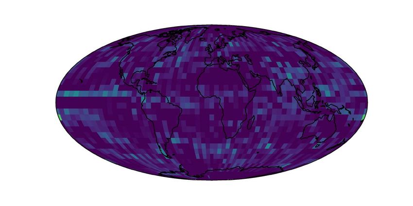
Marine Boundary Layer. Geophysical Research Letters             Saha, M.; Mitra, P.; and Nanjundiah, R. S. 2017. Deep learn-
46(16): 10053–10060. ISSN 1944-8007. doi:10.1029/               ing for predicting the monsoon over the homogeneous re-
2019GL083646.                                                   gions of India. Journal of Earth System Science 126(4): 54.
MetOffice. 2012.         Fact sheet 3 — Water in the            ISSN 0973-774X. doi:10.1007/s12040-017-0838-7. URL
atmosphere.           Technical report, MetOffice UK.           https://doi.org/10.1007/s12040-017-0838-7.
URL           https://www.metoffice.gov.uk/binaries/content/    Saha, M.; Santara, A.; Mitra, P.; Chakraborty, A.; and
assets/metofficegovuk/pdf/research/library-and-                 Nanjundiah, R. S. 2020. Prediction of the Indian sum-
archive/library/publications/factsheets/factsheet 3-water-      mer monsoon using a stacked autoencoder and ensem-
in-the-atmosphere.pdf.                                          ble regression model.   International Journal of Fore-
                                                                casting ISSN 0169-2070. doi:10.1016/j.ijforecast.2020.03.
Mirza, M.; and Osindero, S. 2014. Conditional Generative
                                                                001. URL http://www.sciencedirect.com/science/article/pii/
Adversarial Nets. arXiv:1411.1784 [cs, stat] URL http://
                                                                S0169207020300479.
arxiv.org/abs/1411.1784. ArXiv: 1411.1784.
                                                                Saunders, R.; Hocking, J.; Turner, E.; Rayer, P.; Rundle, D.;
Paszke, A.; Gross, S.; Massa, F.; Lerer, A.; Bradbury, J.;
                                                                Brunel, P.; Vidot, J.; Roquet, P.; Matricardi, M.; Geer, A.;
Chanan, G.; Killeen, T.; Lin, Z.; Gimelshein, N.; Antiga,
                                                                et al. 2018. An update on the RTTOV fast radiative transfer
L.; Desmaison, A.; Kopf, A.; Yang, E.; DeVito, Z.; Raison,
                                                                model (currently at version 12). Geoscientific Model Devel-
M.; Tejani, A.; Chilamkurthy, S.; Steiner, B.; Fang, L.; Bai,
                                                                opment 11(7).
J.; and Chintala, S. 2019. PyTorch: An Imperative Style,
High-Performance Deep Learning Library. In Wallach, H.;         Shorten, C.; and Khoshgoftaar, T. M. 2019. A survey on Im-
Larochelle, H.; Beygelzimer, A.; d. Alché-Buc, F.; Fox, E.;    age Data Augmentation for Deep Learning. Journal of Big
and Garnett, R., eds., Advances in Neural Information Pro-      Data 6(1): 60. ISSN 2196-1115. doi:10.1186/s40537-019-
cessing Systems 32, 8024–8035. Curran Associates, Inc.          0197-0. URL https://doi.org/10.1186/s40537-019-0197-0.
Pinckaers, H.; van Ginneken, B.; and Litjens, G. 2019.          Sønderby, C. K.; Espeholt, L.; Heek, J.; Dehghani, M.;
Streaming convolutional neural networks for end-to-end          Oliver, A.; Salimans, T.; Agrawal, S.; Hickey, J.; and Kalch-
learning with multi-megapixel images. arXiv:1911.04432          brenner, N. 2020. MetNet: A Neural Weather Model for
[cs] URL http://arxiv.org/abs/1911.04432.       ArXiv:          Precipitation Forecasting. arXiv preprint arXiv:2003.12140
1911.04432.                                                     .
Praveen, B.; Talukdar, S.; Shahfahad; Mahato, S.; Mon-          Vogel, E.; Donat, M. G.; Alexander, L. V.; Meinshausen, M.;
dal, J.; Sharma, P.; Islam, A. R. M. T.; and Rahman, A.         Ray, D. K.; Karoly, D.; Meinshausen, N.; and Frieler, K.
2020. Analyzing trend and forecasting of rainfall changes       2019. The effects of climate extremes on global agricultural
in India using non-parametrical and machine learning ap-        yields. Environmental Research Letters 14(5): 054010.
proaches. Scientific Reports 10(1): 10342. ISSN 2045-           Weyn, J. A.; Durran, D. R.; and Caruana, R. 2019. Can Ma-
2322. doi:10.1038/s41598-020-67228-7. URL https://www.          chines Learn to Predict Weather? Using Deep Learning to
nature.com/articles/s41598-020-67228-7. Number: 1 Pub-          Predict Gridded 500-hPa Geopotential Height From Histor-
lisher: Nature Publishing Group.                                ical Weather Data. Journal of Advances in Modeling Earth
Rasp, S.; Dueben, P. D.; Scher, S.; Weyn, J. A.; Mouata-        Systems 11(8): 2680–2693. ISSN 1942-2466.
did, S.; and Thuerey, N. 2020.         WeatherBench: A          Weyn, J. A.; Durran, D. R.; and Caruana, R. 2020.
benchmark dataset for data-driven weather forecasting.          Improving data-driven global weather prediction using
arXiv:2002.00469 [physics, stat] ArXiv: 2002.00469.             deep convolutional neural networks on a cubed sphere.
Rasp, S.; and Thuerey, N. 2020. Purely data-driven medium-      arXiv:2003.11927 [physics, stat] URL http://arxiv.org/abs/
range weather forecasting achieves comparable skill to          2003.11927. ArXiv: 2003.11927.
physical models at similar resolution .                         Xingjian, S.; Chen, Z.; Wang, H.; Yeung, D.-Y.; Wong, W.-
                                                                K.; and Woo, W.-c. 2015. Convolutional LSTM network:
Rezende, D. J.; and Mohamed, S. 2016. Variational Infer-
                                                                A machine learning approach for precipitation nowcasting.
ence with Normalizing Flows. arXiv:1505.05770 [cs, stat]
                                                                In Advances in neural information processing systems, 802–
.
                                                                810.
Rocklin, M. 2015. Dask: Parallel Computation with Blocked
                                                                Zhang, F.; Sun, Y. Q.; Magnusson, L.; Buizza, R.; Lin, S.-
algorithms and Task Scheduling. In Huff, K.; and Bergstra,
                                                                J.; Chen, J.-H.; and Emanuel, K. 2019. What Is the Pre-
J., eds., Proceedings of the 14th Python in Science Confer-
                                                                dictability Limit of Midlatitude Weather? Journal of the At-
ence, 130 – 136.
                                                                mospheric Sciences 76(4): 1077–1091. ISSN 0022-4928.
Rudner, T. G. J.; Rußwurm, M.; Fil, J.; Pelich, R.; Bis-        doi:10.1175/JAS-D-18-0269.1. Publisher: American Mete-
chke, B.; Kopačková, V.; and Biliński, P. 2019. Multi3Net:   orological Society.
Segmenting Flooded Buildings via Fusion of Multireso-           Zsótér, E. 2006. Recent developments in extreme weather
lution, Multisensor, and Multitemporal Satellite Imagery.       forecasting. doi:10.21957/kl9821hnc7. Issue: 107 Pages:
Proceedings of the AAAI Conference on Artificial Intelli-       8-17 Publisher: ECMWF.
gence 33(01): 702–709. ISSN 2374-3468. doi:10.1609/aaai.
v33i01.3301702. Number: 01.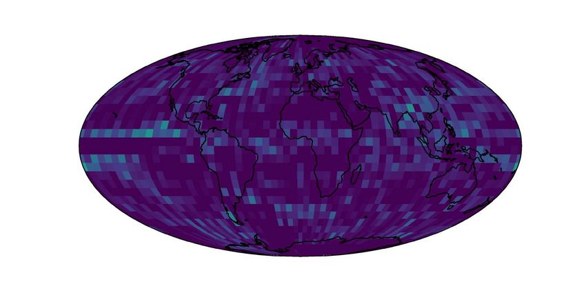
Appendix
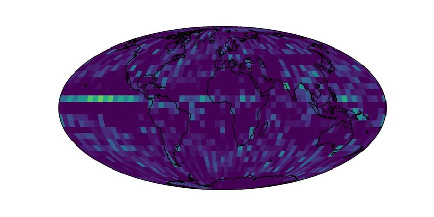
Pixel-wise precipitation class histograms (IMERG)
We include pixel-wise precipitation class histograms derived from IMERG at native resolution (0.1◦ ) with max-pooling as
downscaling to preserve pixel-wise extremes.
90 S 100%
72 S
54 S
98%
36 S
18 S
0 97%
18 N
36 N
96%
54 N
72 N
90 N 95%
180 W 144 W 108 W 72 W 36 W 0 36 E 72 E 108 E 144 E 180 E
Figure 5: Global distribution of slight rain events (% of total events)
90 S 5%
72 S
54 S
3%
36 S
18 S
0 2%
18 N
36 N
1%
54 N
72 N
90 N 0%
180 W 144 W 108 W 72 W 36 W 0 36 E 72 E 108 E 144 E 180 E
Figure 6: Global distribution of moderate rain events (% of total events)90 S 1%
72 S
54 S
0%
36 S
18 S
0 0%
18 N
36 N
0%
54 N
72 N
90 N 0%
180 W 144 W 108 W 72 W 36 W 0 36 E 72 E 108 E 144 E 180 E
Figure 7: Global distribution of heavy rain events (% of total events)
90 N 0.10%
72 N
54 N
0.07%
36 N
18 N
0 0.05%
18 S
36 S
0.03%
54 S
72 S
90 S 0.00%
180 W 144 W 108 W 72 W 36 W 0 36 E 72 E 108 E 144 E 180 E
Figure 8: Global distribution of violent rain events (% of total events)You can also read