Multidimensional Contrast Limited Adaptive Histogram Equalization
←
→
Page content transcription
If your browser does not render page correctly, please read the page content below
Multidimensional Contrast Limited Adaptive Histogram Equalization
                                                                     Vincent Stimper1,2,∗ , Stefan Bauer1 , Ralph Ernstorfer3 ,
                                                                            Bernhard Schölkopf1 and R. Patrick Xian3,∗
                                                              1
                                                                Max Planck Institute for Intelligent Systems, 72072 Tübingen, Germany
                                                           2
                                                             Physics Department, Technical University Munich, 85748 Garching, Germany
                                                              3
                                                                Fritz Haber Institute of the Max Planck Society, 14195 Berlin, Germany
                                                         {vincent.stimper,stefan.bauer,bs}@tue.mpg.de, {ernstorfer,xian}@fhi-berlin.mpg.de
arXiv:1906.11355v1 [eess.IV] 26 Jun 2019

                                                                      Abstract                             adopted example in this class of CE algorithms is the con-
                                                                                                           trast limited adaptive histogram equalization (CLAHE) [3;
                                              Contrast enhancement is an important preprocess-             4], originally formulated in 2D, which performs local ad-
                                           ing technique for improving the performance of down-            justments of image contrast with low noise amplifica-
                                           stream tasks in image processing and computer vi-               tion. The contrast adjustments are interpolated between
                                           sion. Among the existing approaches based on nonlin-            the neighboring rectilinear image patches called kernels
                                           ear histogram transformations, contrast limited adap-           and the spatial adaptivity in CLAHE is achieved through
                                           tive histogram equalization (CLAHE) is a popular                the selection of the kernel size. The intensity range
                                           choice when dealing with 2D images obtained in nat-             of the kernel histogram set by a clip limit restrains the
                                           ural and scientific settings. The recent hardware               noise amplification in the outcome. The use cases of
                                           upgrade in data acquisition systems results in sig-             CLAHE and its variants range from underwater exploration
                                           nificant increase in data complexity, including their           [5], breast cancer detection in X-ray mammography [6;
                                           sizes and dimensions. Measurements of densely sam-              7], video forensics [8] to charging artifact reduction in
                                           pled data higher than three dimensions, usually com-            electron microscopy [9] and multichannel fluorescence mi-
                                           posed of 3D data as a function of external parame-              croscopy [10]. Due to the original formulation, its appli-
                                           ters, are becoming commonplace in various applica-              cations are concentrated almost exclusively in fields and
                                           tions in the natural sciences and engineering. The ini-         instruments producing 2D imagery.
                                           tial understanding of these complex multidimensional
                                           datasets often requires human intervention through                 However, the current data acquisition systems are capa-
                                           visual examination, which may be hampered by the                ble of producing densely sampled image data at three or
                                           varying levels of contrast permeating through the di-           higher dimensions at high rates [11; 12; 13; 14], following
                                           mensions. We show both qualitatively and quanti-                the rapid progress in spectroscopic and imaging methods
                                           tatively that using our multidimensional extension of           in the characterization of materials and biological systems.
                                           CLAHE (MCLAHE) acting simultaneously on all di-                 Sifting through the image piles to identify relevant features
                                           mensions of the datasets allows better visualization            for scientific and engineering applications is becoming an
                                           and discernment of multidimensional image features,             increasingly challenging task. Despite the variety of exper-
                                           as are demonstrated using cases from 4D photoemis-              imental techniques, the parametric changes (with respect
                                           sion spectroscopy and fluorescence microscopy. Our              to time, temperature, pressure, wavelength, concentration,
                                           implementation of multidimensional CLAHE in Ten-                etc.) in the measured system resulting from internal dy-
                                           sorflow is publicly accessible and supports paralleliza-        namics or external perturbations are often translated into
                                           tion with multiple CPUs and various other hardware              intensity changes registered by the imaging detector circuit
                                           accelerators, including GPUs.                                   [15]. Visualizing and accessing the multidimensional im-
                                                                                                           age features (static or dynamic) often begins with human
                                                                                                           visual examination, which are influenced by the contrast
                                           I.       Introduction                                           determined by the detection mechanism, specimen condi-
                                                                                                           tion and instrument resolution. To assist multidimensional
                                           Contrast is instrumental for visual processing and under-       image processing and understanding, the existing CE algo-
                                           standing of the information content within images in var-       rithms formulated in 2D should adapt to the demands of
                                           ious settings [1]. Therefore, computational methods for         higher dimensions (3D and above). Recently, a 3D exten-
                                           contrast enhancement (CE) are frequently used to im-            sion of CLAHE has been described and shown to compare
                                           prove the visibility of images [2]. Among the existing          favorably over separate 2D CLAHE for volumetric (3D)
                                           CE methods, histogram transform-based algorithms are            imaging data both in visual inspection and in a contrast
                                           popular due to their computational efficiency. A widely         metric, the peak signal-to-noise ratio (PSNR) [16].
                                                ∗                                                            In this work, we formulate and implement multidimen-
                                                    Contact Authors

                                                                                                       1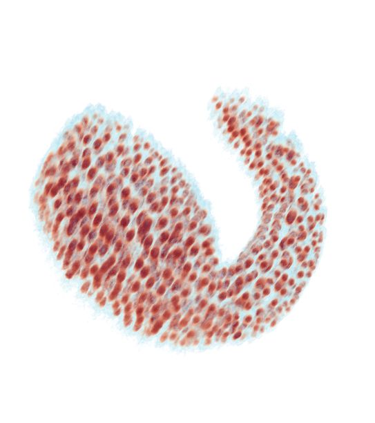
sional CLAHE (MCLAHE), a flexible and efficient frame-               overheads due to the many kernel histograms involved. In
work that generalizes the CLAHE algorithm to an arbi-                performance, the noise in regions with relatively uniform
trary number of dimensions. The MCLAHE algorithm                     intensities tends to be overamplified. Pizer et al. pro-
builds on the principles of CLAHE and, in addition, al-              posed a version of AHE [3] with much less computational
lows the use of arbitrary-shape rectilinear kernels and ex-          cost by using only the adjoining kernels that divide up the
pands the spatial adaptivity of CLAHE to the intensity               image for local histogram computation and intensity map-
domain with adaptive histogram range selection, neither              ping determination, followed by nearest-neighbor interpo-
of which is present in the original formulation of 2D [3;            lation to other pixels not centered on a kernel. Moreover,
4] or 3D CLAHE [16]. Next, we demonstrate the effec-                 they introduced the histogram clip limit to constrain the
tiveness of MCLAHE using visual comparison and compu-                intensity redistribution and suppress noise amplification [3;
tational contrast metrics of two 4D (3D+time) datasets in            4]. The 3D extension of CLAHE was recently introduced by
materials science by photoemission spectroscopy [17] and in          Amorim et al. [16] for medical imaging applications. Their
biological science by fluorescence microscopy [18], respec-          algorithm uses volumetric kernels to compute the local his-
tively. These two techniques are representatives of the cur-         tograms and trilinear interpolation to derive the voxelwise
rent capabilities and complexities of multidimensional data          intensity mappings from nearest-neighbor kernels. Qual-
acquisition methods in natural sciences. The use and adop-           itative results were demonstrated on magnetic resonance
tion of CE in their respective communities will potentially          imaging data, showing that the volumetric CLAHE leads to
benefit visualization and downstream data analysis. Specif-          a better contrast than applying 2D CLAHE separately to
ically, in the photoemission spectroscopy dataset of elec-           every slice of the data. Unfortunately, their code is not in
tronic dynamics in a semiconductor material, we show that            the public domain for further use and testing.
MCLAHE can drastically reduce the intensity anisotropy                  Evaluating the outcome of contrast enhancement re-
and enable visual inspection of dynamical features across            quires quantitative metrics of image contrast, which are
the bandgap; In the fluorescence microscopy dataset of a             rarely used in the early demonstrations of HE algorithms [3;
developing embryo [19], we show that MCLAHE improves
                                                                     22; 24; 25; 26; 27] because the use cases are predom-
the visual discernibility of cellular dynamics from sparse la-       inantly in 2D and the improvements of image quality
beling. In addition, we provide a Tensorflow [20] imple-             are largely intuitive. In domain-specific settings involving
mentation of MCLAHE publicly accessible on GitHub [21],              higher-dimensional (3D and above) imagery, intuition be-
which enables the reuse and facilitates the adoption of the          comes less suitable for making judgments, but computa-
algorithm in a wider community.                                      tional contrast metrics can provide guidance for evalua-
   The outline of the paper is as follows. In Section II,            tion. The commonly known contrast metrics include the
we summarize the developments in histogram equalization              mean squared error (MSE) (or the related PSNR) [28;
leading up to CLAHE and the use of contrast metrics in               29], the standard deviation (or the root-mean-square con-
outcome evaluation. In Section III, we highlight the details         trast) [30] and the Shannon entropy (or the grey-level
of the MCLAHE algorithm that differentiate from previous             entropy) [31]. These metrics are naturally generalizable
lower-dimensional CLAHE algorithms. In Section IV, we                to imagery in arbitrary dimensions [32] and are easy to
describe the use cases of MCLAHE in photoemission spec-              compute. We also note that despite the recently de-
troscopy and fluorescence microscopy. In Section V, we               veloped 2D image quality assessment scores based on
comment on the current limitations and potential improve-            the current understanding of human visual systems [28;
ments in the software implementation. Finally, in Section            31] proved to be more effective than the classic metrics
VI, we draw the conclusions.                                         we choose to quantify contrast, their generalization and
                                                                     relevance to the evaluation of higher-dimensional images
                                                                     obtained in natural sciences and engineering settings, of-
II.   Background and related work                                    ten without undistorted references, are not yet explored, so
                                                                     they are not used here for comparison of results.
Histogram transform-based CE began with the histogram
equalization (HE) algorithm developed by Hall in 1974
[22], where a pixelwise intensity mapping derived from               III.    Methods
the normalized cumulative distribution function (CDF)
of the entire image’s intensity histogram is used to re-             A.     Overview
shape the histogram into a more uniform distribution [22;
23]. However, Hall’s approach derives the intensity his-             Extending CLAHE to multiple dimensions requires to ad-
togram globally, which can overlook fine-scale image fea-            dress some of the existing limitations of the 2D (or 3D)
tures of varying contrast. Subsequent modifications to HE            version of the algorithm. (1) The formulation of 2D [3;
introduced independently by Ketcham [24] and Hummel                  4] and 3D CLAHE [16] involve explicit enumerated treat-
[25], named the adaptive histogram equalization (AHE) [3],           ment of image boundaries, which becomes tedious and un-
addressed this issue by using the intensity histogram of a           scalable in arbitrary dimensions because the number of dis-
rectangular window, called the kernel, or the contextual             tinct boundaries scales exponentially as 3D −1 with respect
region, around each pixel to estimate the intensity map-             to the number of dimensions D. We resolve this issue by
ping. However, AHE comes with significant computational              introducing data padding in MCLAHE as an initial step

                                                                 2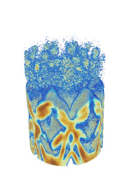
such that every D-dimensional pixel lives in an environ-                  Algorithm 1 Formulation of the MCLAHE procedure in
ment with equal size in the augmented data (see Section                   pseudocode. Here, // denotes the integer division opera-
III.B). The data padding also enables the choice of kernels               tor, cdf the cumulative distribution function, and map the
with an arbitrary size smaller than the original data. (2)                intensity mappings applied to the high dimensional pixels.
The formalism for calculating and interpolating the inten-                Input: data in
sity mapping needs to be generalized to arbitrary dimen-                  Parameters: kernel size (array of integers for all kernel
sions. We present a unified formulation using the Lagrange                dimensions), clip limit (threshold value in [0, 1] for clipping
form of multilinear interpolation [33] that includes the re-              the local histograms), n bins (number of bins of the local
spective use of bilinear and trilinear interpolation in 2D [3;            histograms)
4] and 3D [16] versions of CLAHE as special cases in lower                Output: data out
dimensions (see Section III.C). (3) To further suppress noise              1: pad len = 2 · kernel size - 1 + ((shape(data in) - 1)
amplification in processing image data containing vastly dif-                  mod kernel size)
ferent intensity features, we introduce adaptive histogram                 2: data hist = pad symmetric(data in, [pad len // 2,
range (AHR), which extends the spatial adaptivity of the                       (pad len + 1) // 2])
original CLAHE algorithm to the intensity domain. AHR                      3: b list = split data hist into kernels of size kernel size
allows the choice of local histogram range according to the                4: for each b in b list do
intensity range of each kernel instead of using a global his-              5:    h = histogram(b, n bins)
togram range (GHR) (see Section III.D).                                    6:    Redistribute weight in h above clip limit equally
                                                                                 across h
                                                    For each kernel
                                                                           7:    cdf b = cdf(h)
                Multidimensional      Division        Histogram            8:    map[b] = (cdf b - min(cdf b)) / (max(cdf b) -
     Input
                    padding         into kernels     computation                 min(cdf b))
                                                                           9: end for
                                                      Histogram           10: for each neighboring kernel do
                                                       clipping
                                                                          11:    for each pixel p in data in do
                                                                          12:       u = map[b in neighboring kernel of p](p)
                Multidimensional                    Computation of
     Output
                 interpolation
                                   Apply mappings                         13:       for d = 0 ... D-1 do
                                                    normalized CDF
                                                                          14:         u = u · (coefficient of the neighboring kernel in
                                                                                      dimension d)
         Figure 1: Schematic of the MCLAHE algorithm.                     15:       end for
                                                                          16:       Assign u to pixel p in data out
                                                                          17:    end for
   The MCLAHE algorithm is summarized graphically in                      18: end for
Fig. 1 and in pseudocode in Algorithm 1. It operates                      19: return data out
on input data of dimension D, where D is a positive in-
teger. Let si be the size of data along the ith dimension,
so i ∈ {0, ..., D − 1}. The algorithm begins with padding                 of each kernel is computed with the same number of D-
of the input data around the D-dimensional edges. The                     dimensional pixels. Therefore, the size of the padded data
padded data is then kernelized, or divided into adjoining                 should be an integer multiple of the kernel size. For each
rectilinear kernels with dimension D and a size of bi along               dimension, if si is not an integer multiple of bi , a padding
the ith dimension defined by the user. In each kernel, we                 of bi − (si mod bi ) is needed. To absorb the case when
then separately compute and clip its intensity histogram and              si mod bi ≡ 0, we add a shift of −1 to the expression.
obtain the normalized CDF. The intensity mapping at each                  Therefore, the padding required along the ith dimension
D-dimensional pixel is computed by multilinear interpola-                 of the kernel to make the data size divisible by the kernel
tion of the transformed intensities among the normalized                  size is bi − 1 − ((si − 1) mod bi ). Secondly, we require
CDFs in its nearest-neighbor kernels. Finally, the contrast-              that every D-dimensional pixel in the original data have
enhanced output data is generated by carrying out the same                the same number of nearest-neighbor kernels such that the
procedure for all pixels in the input data.                               pixels at the border do not need a special treatment in the
                                                                          interpolation step. Therefore, we need to pad, in addition,
B.     Multidimensional padding                                           by the kernel size, bi , along the ith dimension. To satisfy
                                                                          both requirements, the total padding length along the ith
Due to the exponential scaling of the distinct boundaries                 dimension, pi , is
as 3D − 1 with the data dimension D, we use multidimen-
sional padding to circumvent the enumerated treatment of                              pi = 2bi − 1 − ((si − 1)     mod bi ).         (1)
boundaries and ensure that the data can be divided into in-               This length is split into two parts, pi0 and pi1 , and attached
teger multiples of the user-defined kernel size. The padding              to the start and end of each dimension, respectively.
is composed of two parts. We discuss the case for D
dimensions and illustrate with an example for D = 2 in                                         pi0 = pi //2,
Fig. 2(c). Firstly, we require that the intensity histogram                                                                          (2)
                                                                                               pi1 = (pi + 1)//2.

                                                                      3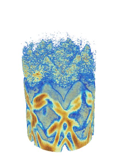
Here, the // sign denotes integer division. To keep the local (0, 0), (0, 1), (1, 0) and (1, 1), as shown in Fig. 2(b). Let
intensity distribution at the border of the image unchanged, mi be the intensity mapping obtained from the kernel with
the paddings are added symmetrically along the boundaries the index i.
of the data. The padding procedure is described in lines mi (In ) = CDF
d i (In ), (3)
1–2 in Algorithm 1.
where CDFi represents the normalized CDF obtained from
d
the clipped histogram of the kernel with the index i. As
(a) (b) shown in Fig. 2(b), the bilinear interpolation at the pixel in
consideration located at the red square mark are computed
using the four nearest-neighbor kernels centered on the blue
square mark. The interpolation coefficients, ci , can be rep-
resented as Lagrange polynomials [34; 33] using the kernel
size (b0 , b1 ) and the distances (d00 , d01 , d10 , d11 ) between
the pixel and the kernel centers in the two dimensions.
(b0 − d00 )(b1 − d10 )
c00 = , (4)
b0 b1
(b0 − d00 )(b1 − d11 )
c01 = , (5)
b0 b1
(c) c10 =
(b0 − d01 )(b1 − d10 )
, (6)
b0 b1
(b0 − d01 )(b1 − d11 )
c11 = . (7)
b0 b1
The transformed intensity I˜n from In is given by
I˜n =c00 m00 (In ) + c01 m01 (In ) + c10 m10 (In )
+ c11 m11 (In ). (8)
Equation (4)-(7) and (8) can be rewritten in a compact
form using the kernel index i introduced earlier,
(9)
X
I˜n = ci mi (In ),
Figure 2: Illustration of the concepts related to the MCLAHE i∈{0,1}2
algorithm in 2D. In (a)-(c) the image is equipartitioned into 1
bj − djij
(10)
Y
kernels of size (b0 , b1 ) bounded by solid black lines. The dotted ci = .
black lines indicate regions with pixels having the same nearest-
j=0
bj
neighbor kernels. Color coding is used to specify the types of
border regions, with the areas in green, orange and magenta In the 2D case, the term djij takes on the value dji0 or
having four, two and one nearest-neighbor kernels, respectively. dji1 . The choice of i0 and i1 from the binary alphabet
A zoomed-in region of (a) is shown in (b). The red square mark {0, 1} in djij follows that of the index i. The special cases
in (b) represents a pixel under consideration and the four blue of transforming the border pixels in the image are naturally
square marks represent the closest kernel centers next to the red resolved in our case after data padding (see Section III.B).
one. The padded image is shown in (c) with the original image
now bounded by solid red lines and the padding is indicated by In D dimensions, the kernel index i = (i0 , i1 , ..., iD−1 ) ∈
the hatchings. The padding lengths in 2D are labeled as p00 , {0, 1}D . Analogous to the two-dimensional case described
p01 , p10 , p11 in (c) and their values are calculated using Eq. (2). before, the intensity mapping of each D-dimensional pixel
is now calculated by multilinear interpolation between the
2D nearest-neighbor kernels in all dimensions.
C. Multidimensional interpolation I˜n =c00...0 m00...0 (In ) + c00...1 m00...1 (In )
(11)
+ c11...0 m11...0 (In ) + c11...1 m11...1 (In ).
To derive a generic expression for the intensity mapping
in arbitrary dimensions, we start with the example in 2D Similarly, (11) and the corresponding expressions for the
CLAHE, where each pixel intensity In (n being the pixel interpolation coefficients can be written in the compact
or voxel index) is transformed by a bilinear interpolation of form as
the mapped intensities obtained from the normalized CDF (12)
X
I˜n = ci mi (In ),
of the nearest-neighbor kernels [3; 4]. We introduce the i∈{0,1}D
kernel index i = (i0 , i1 ) ∈ {0, 1}2 . The values of 0 and 1
in the binary alphabet {0, 1} represent the two sides (i.e. D−1
bj − djij
(13)
Y
above and below) in a dimension divided by the pixel in ci =
bj
.
consideration. For the 2D case, (i0 , i1 ) takes the values of j=0
4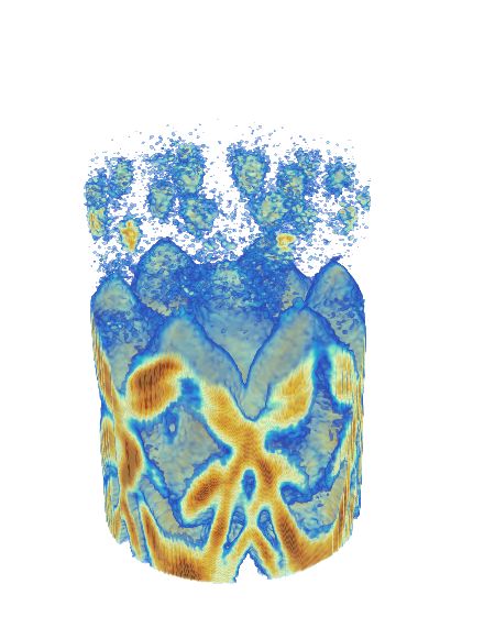
The formalism is very similar to that of the 2D case (see           demarcation of the band-like image features are of great
(8)-(10)), yet allows us to generalize to arbitrary dimension       importance for understanding the momentum-space elec-
with only an update to the kernel index i. In Algorithm 1,          tronic distribution and dynamics in multidimensional pho-
the calculation of intensity mappings through interpolation         toemission spectroscopy [14]. However, in addition to the
is described in lines 12–15.                                        physical limitations on the contrast inhomogeneities listed
                                                                    before, the intensity difference between the lower bands
D.    Adaptive histogram range                                      (or valence bands) and the upper bands (or conduction
                                                                    bands) on the energy scale is on the order of 100 or higher
In the original formulation of CLAHE in 2D [3; 4], the local        and varies by the materials under study and light excita-
histogram ranges for all kernels are the same, which works          tion conditions. To improve the image contrast in multi-
well when the kernels contain intensities in a similarly wide       ple dimensions, we applied MCLAHE to a 4D (3D+time)
range. Tuning of the trade-off between noise amplifica-             dataset measured for the time- and momentum-resolved
tion and the signal enhancement is then achieved through            electron dynamics of tungsten diselenide (WSe2 ), a semi-
the kernel size and the clip limit [29]. However, if differ-        conductor material with highly dispersing electronic bands
ent patches of the image data contain local features within         [36]. The 4D data are obtained from an existing experimen-
distinct narrow intensity ranges, they may accumulate in            tal setup [37] and processed using a custom pipeline [38;
very few histogram bins set globally, which then will re-           39] from registered single photoelectron events. For com-
quire a high clip limit to enhance and therefore comes with         parison of contrast enhancement, we apply both 3D and
the price of noise amplification in many parts of the data.         4D CLAHE to the 4D photoemission spectroscopy data. In
This problem may be ameliorated by adaptively choosing              the case of 3D CLAHE, the algorithm is applied to the 3D
the local histogram range to lie within the minimum and             data at each time frame separately. The raw data and the
maximum of the intensity values of the kernel, while keep-          results are shown in Fig. 3, along with the contrast metrics
ing the number of bins the same for all kernels. An example         computed and listed in Table 1.
use case of the AHR is presented in Section IV.A.
                                                                    Results and discussion. The original photoemission spec-
                                                                    troscopy data are visualized poorly on an energy scale cov-
IV.    Applications                                                 ering both the valence and conduction bands, as shown
                                                                    in Fig. 3(a)-(d). The situation is much improved in the
We now apply the MCLAHE algorithm to two cases in                   MCLAHE-processed data shown in Fig. 3(e)-(l), where the
the natural sciences that involve large densely sampled 4D          population dynamics in the conduction band of WSe2 [40;
(3D+time) data. Each example includes a brief introduc-             41] and the band broadening in the valence bands are suffi-
tion of the background knowledge on the type of measure-            ciently visible to be placed on the same colorscale, allowing
ment, the resulting image data features and the motivation          to identify and correlate fine features of the momentum-
for the use of contrast enhancement, followed by discussion         space dynamics. The improvement is also reflected quanti-
and comparison of the outcome using MCLAHE. The per-                tatively in Table 1 in the drastic increase in MSE and, cor-
formance details are provided at the end of each example.           respondingly, the drop in the PSNR and standard deviation
                                                                    between the unadjusted (smoothed) and contrast-enhanced
A.    Photoemission spectroscopy                                    data. Furthermore, visual comparison of the results in Fig.
                                                                    3(e)-(l) show that noise enhancement is less severe when
Background information. In photoemission spectroscopy,              applying 4D CLAHE though unavoidable to some extend
the detector registers electrons liberated by intense vacuum        due to the weakness of the dynamical signal. This is rep-
UV or X-ray pulses from a solid state material sample [17].         resented in the slight decrease in MSE or, equivalently, the
The measurement is carried out in the so-called 3D momen-           slight increase in PSNR between the 3D and 4D CLAHE-
tum space, spanned by the coordinates (kx , ky , E), in which       processed data. Finally, the processing also compares the
kx , ky are the electron momenta and E the energy. The de-          use of AHR and GHR in dataset including drastically differ-
tected electrons form patterns carrying information about           ent intensity features, which in this case are represented by
the anisotropic electronic density distribution within the          the valence and conduction bands. The inclusion of AHR
material. The fourth dimension in time-resolved photoemis-          compares favorably over GHR (not shown in Fig. 3) in both
sion spectroscopy represent the waiting time in observation         the 3D and 4D scenarios as indicated in the improvement
since the electronic system is subject to an external pertur-       in all contrast metrics in Table 1. The improvement comes
bation (i.e. light excitation). In the image data acquired in       from correctly accounting for the large intensity variations
photoemission spectroscopy, the inhomogeneous intensity             in different regions of the image.
modulation from the experimental geometry, light-matter
interaction [35] and scattering background creates contrast           To quantify the influence of contrast enhancement on
variations within and between the so-called energy bands,           the dynamical features in the data, we calculated the inte-
which manifest themselves as intercrossing band-like curves         grated intensity in the conduction band of the data in all
(in 2D) or surfaces (in 3D) blurred by convolution with the         three cases and the results are summarized in Fig. 3(m)-
instrument response function and further affected by other          (o). The standard score in Fig. 3(o) is used to compare
factors such as the sample quality and the dimensional-             the integrated signals in a scale-independent fashion. The
ity of the electronic system, etc [17]. Visualization and           dynamics represented in the intensity changes are better

                                                                5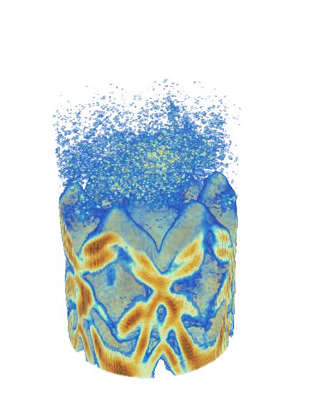
(a)             t1 = -62 fs                         (b)                   t2 = 6 fs                                                (c)               t3 = 52 fs                                 (d)             t4 = 128 fs
         Raw data

                           E

                    kx
                                             ky

                                       (e)                                                 (f)                                                                            (g)                                                          (h)
         3D CLAHE

                                       (i)                                                 (j)                                                                            (k)                                                          (l)
         4D CLAHE

                                                                                                                                                                                                                                                                                      Intensity
                (m)                                                                                              (n)                                                                                     (o)
                                                                                                                                                 t1         t2       t3               t4                                               t1         t2     t3         t4
                                                                                                                                                                                             Raw data                                                                      Raw data
                                                                                                             Integrated intensity (a.u.)

                                   1                                                                                                                                                         3D CLAHE                                                                      3D CLAHE
                                                                                                                                                                                                         Standard score (a.u.)

                                                                                                                                                                                             4D CLAHE                                                                      4D CLAHE
                     Energy (eV)

                                   0

                                   1
                                                                                                 Intensity

                                   2

                                   3

                                   4
                                              1.5    1.0   0.5   0.0   0.5   1.0       1.5                                                 100        50   0         50         100        150    200                            100        50   0      50    100        150    200
                                                                                   1
                                                  Electron momentum kx (Å              )                                                                   Time delay (fs)                                                                       Time delay (fs)

Figure 3: Applications of MCLAHE to 4D (3D+time) photoemission spectroscopy data including the temporal evolution of the
electronic band structure of the semiconductor WSe2 during and after optical excitation (see Section IV.A). Four time steps in the
4D time series are selected for visualization including the raw data in (a)-(d), the 3D CLAHE-processed data in (e)-(h) and the 4D
CLAHE-processed data in (i)-(l). The adaptive histogram range (AHR) setting in the MCLAHE algorithm were included in the data
processing. All 3D-rendered images in (a)-(l) share the same color scaling shown in (l). The integrated dynamics in (n)-(o) over
the region specified by the box in (m) over the 3D momentum space show that the 4D CLAHE amplifies less noise while better
preserves the dynamical timescale than the 3D CLAHE, in comparison with the original data.

                                                                                                                                                                 6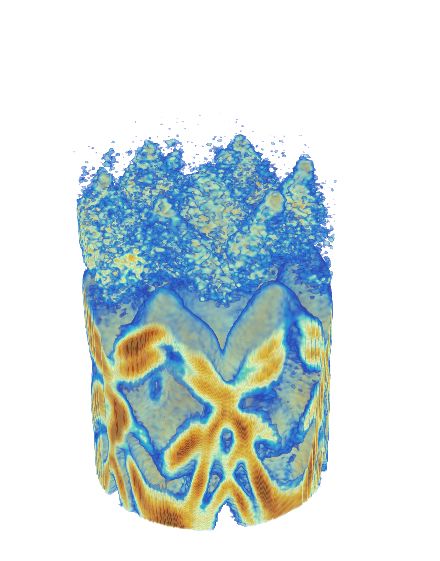
preserved in 4D than 3D CLAHE-treated data and the for-              enhancement method is potentially useful to improve the
mer are less influenced by the boundary artifacts in the             visibility of the cells and their corresponding dynamics. We
beginning and atvthe end of the time delay range. These              demonstrate the use of MCLAHE for this purpose on a
observations reinforce the argument that 4D CLAHE is su-             publicly available 4D (3D+time) fluorescence microscopy
perior to its 3D counterpart overall in content-preserving           dataset [19] of embryo development of the ascidian (Phallu-
contrast enhancement.                                                sia mammillata), or sea squirt. The organism is stained and
                                                                     imaged in toto to reveal its development from a gastrula to
Table 1: Contrast metrics for photoemission spectroscopy data        tailbud formation with cellular resolution [19]. During em-
                                                                     bryo development, the fluorescence contrast exhibits time
     Dataset             MSE      PSNR     STD      ENT              dependence due to cellular processes such as division and
     Raw                 -        -        0.0667   2.294            differentiation. We used the data from one fluorescence
     Smoothed            0.0015   166.63   0.0938   2.615            color channel containing the nuclei and processed through
     3D CLAHE   (GHR)    0.0426   152.18   0.2296   3.048            the MCLAHE pipeline. The results are compared with the
     4D CLAHE   (GHR)    0.0428   152.16   0.2299   3.049            original data on the same colorscale in Fig. 4 and the cor-
     3D CLAHE   (AHR)    0.1121   147.98   0.2838   4.471            responding contrast metrics are shown in Table 2.
     4D CLAHE   (AHR)    0.1050   148.26   0.2818   4.387
                                                                     Results and discussion. The intensities in the raw fluo-
MSE: mean square error. PSNR: peak signal-to-noise ratio.            rescence microscopy data are distributed highly unevenly in
STD: standard deviation. ENT: Shannon entropy.                       the colorscale, as shown in Fig. 4(a)-(d). The MCLAHE-
                                                                     processed 4D time series show significant improvement in
                                                                     the visibility of the cells against the background signal (e.g.
                                                                     autofluorescence, detector dark counts, etc). This is re-
Processing details. The raw 4D photoemission spec-                   flected in the surge in MSE, an increase in standard de-
troscopy data have a size of 180×180×300×80 in the (kx ,             viation and a drop in PSNR as shown in Table 2. In
ky , E, t) dimensions. They are first denoised using a Gaus-         contrast to the previous example, in processing the em-
sian filter with standard deviations of 0.7, 0.9 and 1.3 along       bryo development dataset, the AHR option in MCLAHE
the momenta, energy and time dimensions, respectively.               was not used because the cellular feature sizes and their
For both the application of 3D and 4D CLAHE, we used                 fluorescence intensities are similar throughout the organ-
a clip limit of 0.02 and local histograms with 256 grey-             ism, additionally, the dynamic range of the data is lim-
level bins. The kernel size for 4D CLAHE was (30, 30, 15,            ited (see following discussion in Processing details) and the
20) and for 3D CLAHE the same kernel size for the first              changes in fluorescence during development are relatively
three dimensions, or (kx , ky , E) was used. Both GHR and            small. The initial high Shannon entropy of the raw data
AHR settings were used for comparison. The processing                in Table 2 is due to its high background noise, which is
ran on a server with 64 Intel Xeon CPUs at 2.3 GHz and               reduced after smoothing, as indicated by the sharp drop in
254GB RAM. Running the 4D CLAHE procedure on the                     the entropy while the standard deviation show relative con-
whole dataset took about 5.3 mins. In addition, we bench-            sistency. Then, the use of MCLAHE increases the entropy
marked the performance of 4D CLAHE on a GPU (NVIDIA                  again, together with the large changes in other metrics,
GeForce GTX 1070, 8GB RAM) connected to the same                     this time due to the contrast enhancement. Similarly to
server by processing the first 25 time frames of the dataset.        the previous example, the 4D CLAHE outperforms its 3D
The processing took 34 s versus 104 s when using the 64              counterpart overall because of the lower MSE or, equiv-
CPUs only, which represents a 3.1-fold speed-up.                     alently, the higher PSNR of the 4D results, indicating a
                                                                     higher similarity to the raw data. In other contrast metrics
B.    Fluorescence microscopy                                        such as the standard deviation and the Shannon entropy,
                                                                     the 4D and 3D results have very close values, indicating the
Background information. In 4D fluorescence microscopy,               complexity of judging image contrast by a single metric. Vi-
the measurements are carried out in the Cartesian coordi-            sualization of the dynamics in Fig. 4(e)-(l) also shows that
nates of the laboratory frame, or (x, y, z), with the fourth         the 4D CLAHE-processed data preserve more of the fluo-
dimension representing the observation time t. In prac-              rescence intensity change than its 3D counterpart, which
tice, the photophysics of the fluorophores [42], the aut-            still maintaining a high cell-to-background contrast. The
ofluorescence background [18] from the unlabeled part of             contrast-enhanced embryo development data potentially al-
the sample and the detection method, such as attenuation             lows better tracking of cellular lineage and dynamics [45;
effect from scanning measurements at different depths or             46] that are challenging due to sparse fluorescent labeling.
nonuniform illumination of fluorophores [43], pose a limit
on the achievable image contrast in the experiment. The
image features in fluorescence microscopy data often in-             Processing details. The raw 4D fluorescence microscopy
clude sparsely labeled cells and cellular components such            data have a size of 512×512×109×144 in the (x, y, z, t)
as the nuclei, organelles, membrane or dendrite structures.          dimensions. They are first denoised by a median filter with
The limited contrast may render the downstream data an-              the kernel size (2, 2, 2, 1). For 4D CLAHE, the kernel
notation tasks, such as segmentation, tracking and lineage           size of choice was (20, 20, 10, 25) and the same kernel
tracing [44; 45], challenging. Therefore, a digital contrast         size in the first three dimensions were used for 3D CLAHE

                                                                 7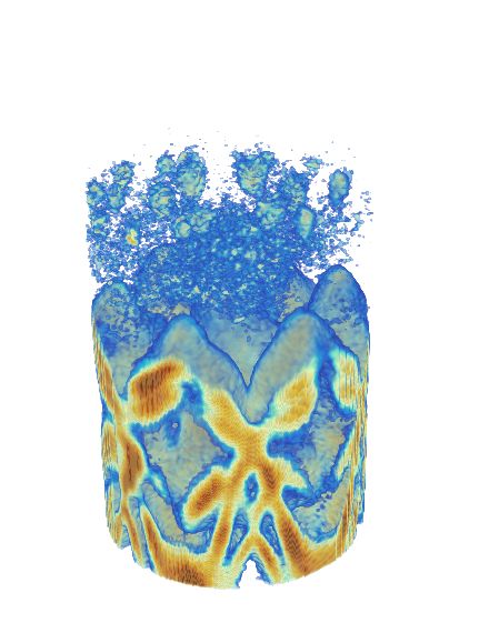
(a) t1 = 5.75 hpf (b) t2 = 7.25 hpf (c) t3 = 8.5 hpf (d) t4 = 10 hpf
Raw data
z
x
y
(e) (f) (g) (h)
3D CLAHE
(i) (j) (k) (l)
4D CLAHE
Intensity
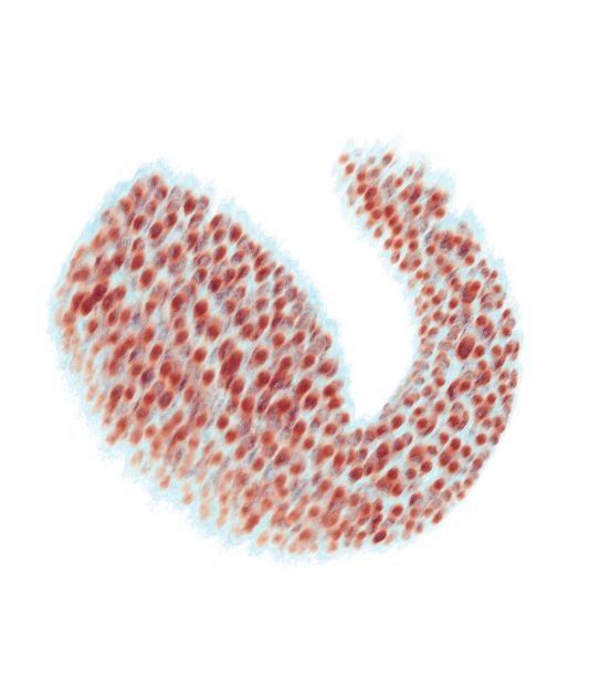
Figure 4: Applications of MCLAHE to 4D (3D+time) fluorescence microscopy data of the embryo development of ascidian (Phallusia
mammillata), or sea squirt. Four time frames (hpf = hours post fertilization) in the 4D time series are visualized here for comparison,
including the raw data in (a)-(d), the 3D CLAHE-processed data in (e)-(h) and the 4D CLAHE-processed data in (i)-(l). All images
in (a)-(l) are rendered in 3D with the same color scaling shown in (l). Both MCLAHE-processed data show drastic improvement in
the image contrast, while 4D CLAHE-processed data better preserves the dynamical intensity features from cellular processes.
8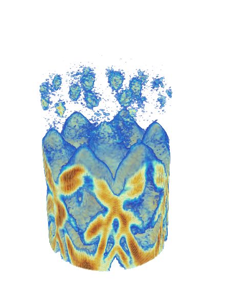
Table 2: Contrast metrics for fluorescence microscopy data         contrast quantification in case studies drawn from differ-
                                                                     ent measurement techniques with the capabilities of pro-
 Dataset        MSE(×10−3 )      PSNR     STD       ENT              ducing densely sampled high dimensional data, namely,
 Raw            -                -        0.0316    1.1284           4D (3D+time) photoemission spectroscopy and 4D fluores-
 Smoothed       0.300            173.7    0.0265    0.5141           cence microscopy. In the example applications, our algo-
 3D CLAHE       7.767            159.6    0.1048    0.5262           rithm greatly improves and balances the visibility of image
 4D CLAHE       5.667            160.9    0.0921    0.5241           features in diverse intensity ranges and neighborhood con-
                                                                     ditions. We further show that the best overall performance
                                                                     in each case comes from simultaneous application of multi-
to allow a direct comparison. For both procedures, the
                                                                     dimensional CLAHE to all data dimensions. In addition, we
clip limit was set at 0.25 and the number of histogram
                                                                     provide the implementation of multidimensional CLAHE in
bins at 256. The intensities in the raw data were given
                                                                     an open-source codebase to assist its reuse and integration
as 8 bit unsigned integers resulting in only 256 possible
                                                                     into existing image analysis pipelines in various domains of
values. Hence, only the GHR setting was used because the
                                                                     natural sciences and engineering.
AHR setting would result in bins smaller than the resolution
of the data. Processing using MCLAHE ran on the same
server as for the photoemission spectroscopy data. The               Acknowledgments
runtime using the 64 CPUs was about 26 mins. With the
same setting as in the photoemission case study, processing          We thank the S. Schülke, G. Schnapka at the GNZ
of the first 8 time frames of the dataset took 32 s on the           (Gemeinsames Netzwerkzentrum) in Berlin and M. Rampp
same GPU used previously versus 85 s on 64 CPUs, which               at the MPCDF (Max Planck Computing and Data Facility)
represents a 2.7-fold speed-up.                                      in Garching for computing supports. We thank S. Dong
                                                                     and S. Beaulieu for performing the photoemission spec-
                                                                     troscopy measurement on tungsten diselenide at the Fritz
V.    Perspectives                                                   Haber Institute. V. Stimper thanks U. Gerland for admin-
                                                                     istrative support. The work has received funding from the
While we have presented the applications of the MCLAHE               Max Planck Society, including BiGmax, the Max Planck
algorithm to real-world datasets of up to multiple gigabytes         Society’s Research Network on Big-Data-Driven Materials
in size, its current major performance limitation is in the          Science, and funding from the European Research Council
memory usage, since the data needs to be loaded entirely             (ERC) under the European Union’s Horizon 2020 research
into the RAM (of CPUs or GPUs), which may be challeng-               and innovation program (Grant Agreement No. ERC-2015-
ing for very large imaging and spectroscopy datasets on              CoG-682843).
the multi-terabyte scale that are becoming widely available
[11]. Future improvements on the algorithm implementa-
tion may include distributed handling of chunked datasets            References
to enable operation on hardware with the RAM to load only
                                                                     [1] B. Olshausen and D. Field, “Vision and the
a subset of the data. In addition, the number of nearest-
neighbor kernels currently required for intensity mapping in-            coding of natural images,” American Scientist,
terpolation increases exponentially with the number of data              vol. 88, no. 3, p. 238, 2000. [Online]. Available:
dimension D (see Section III.C). For datasets with D < 10,               http://www.americanscientist.org/issues/feature/
this may not pose a outstanding issue, but for even higher-              2000/3/vision-and-the-coding-of-natural-images
dimensional datasets, new strategies may be developed for            [2] W. K. Pratt, Digital Image Processing, 4th ed. Wiley-
approximate interpolation of selected neighboring kernels                Interscience, 2007.
to alleviate the exponential scaling.                                [3] S. M. Pizer, E. P. Amburn, J. D. Austin,
   Moreover, the applications of MCLAHE are not limited                  R. Cromartie, A. Geselowitz, T. Greer, B. ter
by the examples given in this work but are open to other                 Haar Romeny, J. B. Zimmerman, and K. Zuiderveld,
types of data. It is especially beneficial to preprocessing of           “Adaptive histogram equalization and its variations,”
high dimensional data with dense sampling produced by var-               Computer Vision, Graphics, and Image Processing,
ious fast volumetric spectroscopic and imaging techniques                vol. 39, no. 3, pp. 355–368, 1987. [Online].
[47; 48; 49; 50; 51] for improving the performance of feature            Available:     http://www.sciencedirect.com/science/
annotation and extraction tasks.                                         article/pii/S0734189X8780186X
                                                                     [4] K. Zuiderveld, “Contrast limited adaptive histogram
                                                                         equalization,” in Graphics Gems. Elsevier, 1994,
VI.    Conclusion                                                        pp. 474–485. [Online]. Available: https://linkinghub.
We present a flexible framework to extend the CLAHE al-                  elsevier.com/retrieve/pii/B9780123361561500616
gorithm to arbitrary dimensions for contrast enhancement             [5] M. S. Hitam, W. N. J. H. W. Yussof, E. A.
of complex multidimensional imaging and spectroscopy                     Awalludin, and Z. Bachok, “Mixture contrast limited
datasets. We demonstrate the effectiveness of our algo-                  adaptive histogram equalization for underwater image
rithm, the multidimensional CLAHE, by visual analysis and                enhancement,” in 2013 International Conference

                                                                 9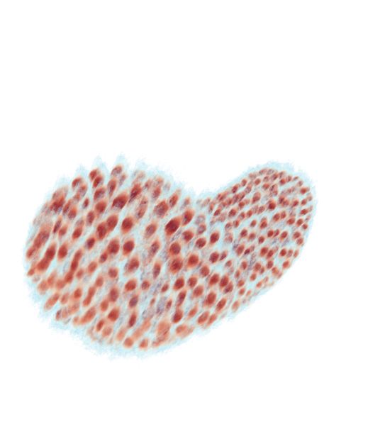
on Computer Applications Technology (ICCAT).                   [15] J. H. Moore, C. C. Davis, M. A. Coplan, and S. C.
     IEEE, jan 2013, pp. 1–5. [Online]. Available:                       Greer, Building Scientific Apparatus, 4th ed. Cam-
     http://ieeexplore.ieee.org/document/6522017/                        bridge University Press, 2009.
[6] W. Morrow, R. Paranjape, R. Rangayyan, and                      [16] P. Amorim, T. Moraes, J. Silva, and H. Pedrini,
    J. Desautels, “Region-based contrast enhancement of                  “3D Adaptive Histogram Equalization Method for
    mammograms,” IEEE Transactions on Medical Imag-                      Medical Volumes,” in Proceedings of the 13th
    ing, vol. 11, no. 3, pp. 392–406, 1992. [Online]. Avail-             International Joint Conference on Computer Vision,
    able: http://ieeexplore.ieee.org/document/158944/                    Imaging and Computer Graphics Theory and Appli-
                                                                         cations. SciTePress, 2018, pp. 363–370. [Online].
[7] E. D. Pisano, S. Zong, B. M. Hemminger,                              Available: http://www.scitepress.org/DigitalLibrary/
    M. DeLuca, R. E. Johnston, K. Muller, M. P.                          Link.aspx?doi=10.5220/0006615303630370
    Braeuning, and S. M. Pizer, “Contrast limited                   [17] S. Hüfner, Photoelectron Spectroscopy : Principles
    adaptive histogram equalization image processing to
                                                                         and Applications, 3rd ed. Springer, 2003.
    improve the detection of simulated spiculations in
    dense mammograms,” Journal of Digital Imaging,                  [18] U. Kubitscheck, Ed., Fluorescence Microscopy:
    vol. 11, no. 4, p. 193, Nov 1998. [Online]. Available:               From Principles to Biological Applications, 2nd ed.
    https://doi.org/10.1007/BF03178082                                   Weinheim, Germany: Wiley-VCH Verlag GmbH
                                                                         & Co. KGaA, may 2017. [Online]. Available:
[8] J. Xiao, S. Li, and Q. Xu, “Video-Based                              http://doi.wiley.com/10.1002/9783527687732
    Evidence Analysis and Extraction in Digital
    Forensic Investigation,” IEEE Access, vol. 7,                   [19] E. Faure, T. Savy, B. Rizzi, C. Melani, O. Stašová,
    pp. 55 432–55 442, 2019. [Online]. Available:                        D. Fabrèges, R. Špir, M. Hammons, R. Čúnderlı́k,
    https://ieeexplore.ieee.org/document/8700194/                        G. Recher, B. Lombardot, L. Duloquin, I. Colin,
                                                                         J. Kollár, S. Desnoulez, P. Affaticati, B. Maury,
[9] K. Sim, Y. Tan, M. Lai, C. Tso, and W. Lim, “Reduc-                  A. Boyreau, J.-Y. Nief, P. Calvat, P. Vernier,
    ing scanning electron microscope charging by using                   M. Frain, G. Lutfalla, Y. Kergosien, P. Suret,
    exponential contrast stretching technique on post-                   M. Remešı́ková, R. Doursat, A. Sarti, K. Mikula,
    processing images,” Journal of Microscopy, vol. 238,                 N. Peyriéras, and P. Bourgine, “A workflow to
    no. 1, pp. 44–56, apr 2010. [Online]. Available: http:               process 3D+time microscopy images of developing
    //doi.wiley.com/10.1111/j.1365-2818.2009.03328.x                     organisms and reconstruct their cell lineage,” Nature
[10] A. McCollum and W. Clocksin, “Multidimensional                      Communications, vol. 7, no. 1, p. 8674, apr 2016.
     histogram equalization and modification,” in 14th                   [Online]. Available: http://www.nature.com/articles/
     International Conference on Image Analysis and                      ncomms9674
     Processing (ICIAP 2007). IEEE, sep 2007, pp.                   [20] M. Abadi, A. Agarwal, P. Barham, E. Brevdo,
     659–664. [Online]. Available: http://ieeexplore.ieee.               Z. Chen, C. Citro, G. S. Corrado, A. Davis, J. Dean,
     org/document/4362852/                                               M. Devin, S. Ghemawat, I. Goodfellow, A. Harp,
                                                                         G. Irving, M. Isard, Y. Jia, R. Jozefowicz, L. Kaiser,
[11] W. Ouyang and C. Zimmer, “The imaging tsunami:                      M. Kudlur, J. Levenberg, D. Mané, R. Monga,
     Computational opportunities and challenges,” Current                S. Moore, D. Murray, C. Olah, M. Schuster,
     Opinion in Systems Biology, vol. 4, pp. 105–113, aug                J. Shlens, B. Steiner, I. Sutskever, K. Talwar,
     2017. [Online]. Available: https://linkinghub.elsevier.             P. Tucker, V. Vanhoucke, V. Vasudevan, F. Viégas,
     com/retrieve/pii/S2452310017300537                                  O. Vinyals, P. Warden, M. Wattenberg, M. Wicke,
[12] P. Pantazis and W. Supatto, “Advances in whole-                     Y. Yu, and X. Zheng, “TensorFlow: Large-scale
     embryo imaging:      a quantitative transition is                   machine learning on heterogeneous systems,” 2015,
     underway,” Nature Reviews Molecular Cell Biology,                   software available from tensorflow.org. [Online].
     vol. 15, no. 5, pp. 327–339, may 2014. [Online].                    Available: http://tensorflow.org/
     Available: http://www.nature.com/articles/nrm3786              [21] V. Stimper and R. P. Xian, “Multidimensional con-
[13] O. Ersen, I. Florea, C. Hirlimann, and C. Pham-                     trast limited adaptive histogram equalization,” https:
     Huu, “Exploring nanomaterials with 3D electron                      //github.com/VincentStimper/mclahe, 2019.
     microscopy,” Materials Today, vol. 18, no. 7, pp. 395–         [22] E. L. Hall, “Almost uniform distributions for computer
     408, sep 2015. [Online]. Available: https://linkinghub.             image enhancement,” IEEE Transactions on Comput-
     elsevier.com/retrieve/pii/S1369702115001200                         ers, vol. C-23, no. 2, pp. 207–208, Feb 1974.
[14] G. Schönhense, K. Medjanik, and H.-J. Elmers,                 [23] P. K. Sinha, Image Acquisition and Preprocessing for
     “Space-, time- and spin-resolved photoemission,”                    Machine Vision Systems. SPIE press, 2012.
     Journal of Electron Spectroscopy and Related                   [24] D. J. Ketcham, “Real-time image enhancement
     Phenomena, vol. 200, pp. 94–118, apr 2015.                          techniques,” in Seminar on Image Processing,
     [Online]. Available: http://linkinghub.elsevier.com/                vol. 0074, 1976, pp. 1–6. [Online]. Available:
     retrieve/pii/S0368204815001243                                      https://doi.org/10.1117/12.954708

                                                               10
[25] R. Hummel, “Image enhancement by histogram Phenomena, vol. 214, pp. 29–52, jan 2017. [Online].
transformation,” Computer Graphics and Image Available: https://linkinghub.elsevier.com/retrieve/
Processing, vol. 6, no. 2, pp. 184 – 195, 1977. pii/S0368204816301724
[Online]. Available: http://www.sciencedirect.com/ [36] J. M. Riley, F. Mazzola, M. Dendzik, M. Michiardi,
science/article/pii/S0146664X77800117 T. Takayama, L. Bawden, C. Granerød, M. Lean-
[26] R. Dale-Jones and T. Tjahjadi, “A study and modifi- dersson, T. Balasubramanian, M. Hoesch, T. K.
cation of the local histogram equalization algorithm,” Kim, H. Takagi, W. Meevasana, P. Hofmann,
Pattern Recognition, vol. 26, no. 9, pp. 1373–1381, M. S. Bahramy, J. W. Wells, and P. D. C. King,
sep 1993. [Online]. Available: https://linkinghub. “Direct observation of spin-polarized bulk bands in an
elsevier.com/retrieve/pii/003132039390143K inversion-symmetric semiconductor,” Nature Physics,
[27] J. Stark, “Adaptive image contrast enhancement vol. 10, no. 11, pp. 835–839, nov 2014. [Online]. Avail-
using generalizations of histogram equalization,” able: http://www.nature.com/articles/nphys3105
IEEE Transactions on Image Processing, vol. 9, [37] M. Puppin, Y. Deng, C. W. Nicholson, J. Feldl,
no. 5, pp. 889–896, may 2000. [Online]. Available: N. B. M. Schröter, H. Vita, P. S. Kirchmann, C. Mon-
http://ieeexplore.ieee.org/document/841534/ ney, L. Rettig, M. Wolf, and R. Ernstorfer, “Time-
[28] Z. Wang, A. Bovik, H. Sheikh, and E. Simoncelli, and angle-resolved photoemission spectroscopy of
solids in the extreme ultraviolet at 500 kHz repetition
“Image quality assessment: From error visibility to
rate,” Review of Scientific Instruments, vol. 90,
structural similarity,” IEEE Transactions on Image
no. 2, p. 023104, feb 2019. [Online]. Available:
Processing, vol. 13, no. 4, pp. 600–612, apr
http://aip.scitation.org/doi/10.1063/1.5081938
2004. [Online]. Available: http://ieeexplore.ieee.org/
document/1284395/ [38] R. P. Xian, L. Rettig, and R. Ernstorfer, “Symmetry-
[29] G. F. C. Campos, S. M. Mastelini, G. J. Aguiar, guided nonrigid registration: The case for distortion
correction in multidimensional photoemission spec-
R. G. Mantovani, L. F. de Melo, and S. Barbon,
troscopy,” Ultramicroscopy, vol. 202, pp. 133–139, jul
“Machine learning hyperparameter selection for
2019. [Online]. Available: https://linkinghub.elsevier.
contrast limited adaptive histogram Equalization,”
com/retrieve/pii/S0304399118303474
EURASIP Journal on Image and Video Processing,
vol. 2019, no. 1, p. 59, dec 2019. [Online]. [39] R. P. Xian, Y. Acremann, S. Y. Agustsson,
Available: https://jivp-eurasipjournals.springeropen. M. Dendzik, K. Bühlmann, D. Curcio, D. Kut-
com/articles/10.1186/s13640-019-0445-4 nyakhov, F. Pressacco, M. Heber, S. Dong, J. Dem-
[30] E. Peli, “Contrast in complex images,” Journal sar, W. Wurth, P. Hofmann, M. Wolf, L. Rettig, and
R. Ernstorfer, “A distributed workflow for volumetric
of the Optical Society of America A, vol. 7,
band mapping data in multidimensional photoemission
no. 10, p. 2032, oct 1990. [Online]. Avail-
spectroscopy,” to be submitted, 2019.
able: https://www.osapublishing.org/abstract.cfm?
URI=josaa-7-10-2032 [40] R. Bertoni, C. W. Nicholson, L. Waldecker,
[31] K. Gu, G. Zhai, W. Lin, and M. Liu, “The H. Hübener, C. Monney, U. De Giovannini,
M. Puppin, M. Hoesch, E. Springate, R. T. Chapman,
analysis of image contrast: From quality assessment
C. Cacho, M. Wolf, A. Rubio, and R. Ernstorfer,
to automatic enhancement,” IEEE Transactions on
“Generation and evolution of spin-, valley-, and
Cybernetics, vol. 46, no. 1, pp. 284–297, jan
layer-polarized excited carriers in inversion-symmetric
2016. [Online]. Available: http://ieeexplore.ieee.org/
WSe2 ,” Physical Review Letters, vol. 117, no. 27,
document/7056527/
p. 277201, dec 2016. [Online]. Available: https:
[32] A. Kriete, “Image quality considerations in computer- //link.aps.org/doi/10.1103/PhysRevLett.117.277201
ized 2-D and 3-D microscopy,” in Multidimensional [41] M. Puppin, “Time- and angle-resolved photoemission
Microscopy. New York, NY: Springer New York,
spectroscopy on bidimensional semiconductors with
1994, pp. 209–230. [Online]. Available: http://link.
a 500 kHz extreme ultraviolet light source,” Ph.D.
springer.com/10.1007/978-1-4613-8366-6{ }12
dissertation, Free University of Berlin, sep 2017.
[33] G. M. Phillips, Interpolation and Approximation [Online]. Available: https://refubium.fu-berlin.de/
by Polynomials, ser. CMS Books in Mathematics. handle/fub188/23006?show=full
New York, NY: Springer New York, 2003. [Online]. [42] B. Valeur and M. N. Berberan-Santos,
Available: http://link.springer.com/10.1007/b97417 Molecular Fluorescence: Principles and Ap-
[34] E. Kreyszig, H. Kreyszig, and E. J. Norminton, Ad- plications, 2nd ed. Wiley-VCH, 2013. [On-
vanced Engineering Mathematics, 10th ed. Wiley, line]. Available: https://www.wiley.com/en-us/
2011. Molecular+Fluorescence{%}3A+Principles+and+
[35] S. Moser, “An experimentalist’s guide to the Applications{%}2C+2nd+Edition-p-9783527328376
matrix element in angle resolved photoemission,” [43] J. C. Waters, “Accuracy and precision in quantitative
Journal of Electron Spectroscopy and Related fluorescence microscopy,” The Journal of Cell Biology,
11vol. 185, no. 7, pp. 1135–1148, jun 2009. [Online].
Available: http://www.jcb.org/lookup/doi/10.1083/
jcb.200903097
[44] T. A. Nketia, H. Sailem, G. Rohde, R. Machiraju, and
J. Rittscher, “Analysis of live cell images: Methods,
tools and opportunities,” Methods, vol. 115, pp. 65–
79, feb 2017. [Online]. Available: https://linkinghub.
elsevier.com/retrieve/pii/S104620231730083X
[45] K. Kretzschmar and F. M. Watt, “Lineage tracing,”
Cell, vol. 148, no. 1-2, pp. 33–45, jan 2012. [Online].
Available: https://linkinghub.elsevier.com/retrieve/
pii/S0092867412000037
[46] F. Amat, W. Lemon, D. P. Mossing, K. McDole,
Y. Wan, K. Branson, E. W. Myers, and P. J. Keller,
“Fast, accurate reconstruction of cell lineages from
large-scale fluorescence microscopy data,” Nature
Methods, vol. 11, no. 9, pp. 951–958, sep 2014.
[Online]. Available: http://www.nature.com/articles/
nmeth.3036
[47] D. J. Flannigan and A. H. Zewail, “4D electron
microscopy: principles and applications,” Accounts
of Chemical Research, vol. 45, no. 10, pp.
1828–1839, oct 2012. [Online]. Available: http:
//pubs.acs.org/doi/10.1021/ar3001684
[48] G. Lu and B. Fei, “Medical hyperspectral imag-
ing: a review,” Journal of Biomedical Optics,
vol. 19, no. 1, p. 010901, jan 2014. [Online].
Available: http://biomedicaloptics.spiedigitallibrary.
org/article.aspx?doi=10.1117/1.JBO.19.1.010901
[49] W. Jahr, B. Schmid, C. Schmied, F. O. Fahrbach, and
J. Huisken, “Hyperspectral light sheet microscopy,”
Nature Communications, vol. 6, no. 1, p. 7990, nov
2015. [Online]. Available: http://www.nature.com/
articles/ncomms8990
[50] A. Özbek, X. L. Deán-Ben, and D. Razansky,
“Optoacoustic imaging at kilohertz volumetric frame
rates,” Optica, vol. 5, no. 7, p. 857, jul 2018.
[Online]. Available: https://www.osapublishing.org/
abstract.cfm?URI=optica-5-7-857
[51] M. K. Miller and R. G. Forbes, Atom-Probe
Tomography. Boston, MA: Springer US, 2014. [On-
line]. Available: http://link.springer.com/10.1007/
978-1-4899-7430-3
12You can also read