MULTIDIMENSIONAL CONTRAST LIMITED ADAPTIVE HISTOGRAM EQUALIZATION - MPG.PURE
←
→
Page content transcription
If your browser does not render page correctly, please read the page content below
Received September 12, 2019, accepted October 15, 2019, date of publication November 11, 2019,
date of current version November 25, 2019.
Digital Object Identifier 10.1109/ACCESS.2019.2952899

Multidimensional Contrast Limited Adaptive
Histogram Equalization
VINCENT STIMPER1,2 , STEFAN BAUER1 , RALPH ERNSTORFER3 ,
BERNHARD SCHÖLKOPF1 , (Senior Member, IEEE), AND RUI PATRICK XIAN                                                            3,4
1 Max   Planck Institute for Intelligent Systems, 72076 Tübingen, Germany
2 Physics Department, Technical University Munich, 85748 Garching, Germany
3 Fritz Haber Institute of the Max Planck Society, 14195 Berlin, Germany
4 Department of Neurobiology, Northwestern University, Evanston, IL 60208, USA

Corresponding authors: Vincent Stimper (vincent.stimper@tuebingen.mpg.de) and Rui Patrick Xian (xian@fhi-berlin.mpg.de)
The work has received funding from the Max Planck Society, including BiGmax, the Max Planck Society’s Research Network on
Big-Data-Driven Materials Science, and funding from the European Research Council (ERC) under the European Union’s Horizon 2020
research and innovation program (Grant Agreement No. ERC-2015-CoG-682843).

  ABSTRACT Contrast enhancement is an important preprocessing technique for improving the performance
  of downstream tasks in image processing and computer vision. Among the existing approaches based
  on nonlinear histogram transformations, contrast limited adaptive histogram equalization (CLAHE) is a
  popular choice for dealing with 2D images obtained in natural and scientific settings. The recent hardware
  upgrade in data acquisition systems results in significant increase in data complexity, including their sizes
  and dimensions. Measurements of densely sampled data higher than three dimensions, usually composed
  of 3D data as a function of external parameters, are becoming commonplace in various applications in the
  natural sciences and engineering. The initial understanding of these complex multidimensional datasets often
  requires human intervention through visual examination, which may be hampered by the varying levels of
  contrast permeating through the dimensions. We show both qualitatively and quantitatively that using our
  multidimensional extension of CLAHE (MCLAHE) simultaneously on all dimensions of the datasets allows
  better visualization and discernment of multidimensional image features, as demonstrated using cases from
  4D photoemission spectroscopy and fluorescence microscopy. Our implementation of multidimensional
  CLAHE in Tensorflow is publicly accessible and supports parallelization with multiple CPUs and various
  other hardware accelerators, including GPUs.

  INDEX TERMS Contrast enhancement, histogram equalization, multidimensional data analysis, photoe-
  mission spectroscopy, fluorescence microscopy.

I. INTRODUCTION                                                                                which performs local adjustments of image contrast with low
Contrast is instrumental for visual processing and under-                                      noise amplification. The contrast adjustments are interpolated
standing of the information content within images in various                                   between the neighboring rectilinear image patches called ker-
settings [1]. Therefore, computational methods for contrast                                    nels and the spatial adaptivity in CLAHE is achieved through
enhancement (CE) are frequently used to improve the vis-                                       selection of the kernel size. The intensity range of the kernel
ibility of images [2]. Among the existing CE methods,                                          histogram (or local histogram) is set by a clip limit that
histogram transform-based algorithms are popular due to                                        restrains the noise amplification in the outcome. Accounts
their computational efficiency. Natural images with a high                                     of the historical development are given in Section II. The
contrast often contain a balanced intensity histogram, this                                    use cases of CLAHE and its variants range from underwater
conception led to the development of histogram equaliza-                                       exploration [6], breast cancer detection in X-ray mammogra-
tion (HE) [3]. A widely adopted example in this class of                                       phy [7], [8], biometric authentication [9], video forensics [10]
CE algorithms is the contrast limited adaptive histogram                                       to charging artifact reduction in electron microscopy [11]
equalization (CLAHE) [4], [5], originally formulated in 2D,                                    and multichannel fluorescence microscopy [12]. Due to
                                                                                               the original formulation, its applications are concentrated
   The associate editor coordinating the review of this manuscript and                         almost exclusively in fields and instruments producing
approving it for publication was Madhu S. Nair            .                                    2D imagery.

                     This work is licensed under a Creative Commons Attribution 4.0 License. For more information, see http://creativecommons.org/licenses/by/4.0/
VOLUME 7, 2019                                                                                                                                                       165437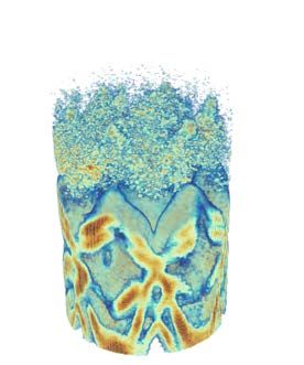
V. Stimper et al.: Multidimensional CLAHE

   However, the current data acquisition systems are capa-         of dynamical features across the bandgap. In the fluorescence
ble of producing densely sampled image data at three or            microscopy dataset of a developing embryo [22], we show
higher dimensions at high rates [13]–[17], following the rapid     that MCLAHE improves the visual discernibility of cellular
progress in spectroscopic and imaging methods in the charac-       dynamics from sparse labeling. In addition, we provide a Ten-
terization of materials and biological systems. Sifting through    sorflow [23] implementation of MCLAHE publicly accessi-
the image piles to identify relevant features for scientific and   ble on GitHub [24], which enables the reuse and facilitates
engineering applications is becoming an increasingly chal-         the adoption of the algorithm in a wider community.
lenging task. Despite the variety of experimental techniques,         The outline of the paper is as follows. In Section II,
the parametric dependence (with respect to time, temperature,      we highlight the developments in histogram equalization
pressure, wavelength, concentration, etc.) in the measured         leading up to CLAHE and the use of contrast metrics in
system resulting from internal dynamics or external perturba-      outcome evaluation. In Section III, we go into detail on
tions are often translated into intensity changes registered by    the differentiators of the MCLAHE algorithm from previ-
the imaging detector circuit [18]. Visualizing and extracting      ous lower-dimensional CLAHE algorithms. In Section IV,
multidimensional image features from acquired data often           we describe the use cases of MCLAHE on 4D photoemission
begin with human visual examination, which is influenced           spectroscopy and fluorescence microscopy data. In Section V,
by the contrast determined by the detection mechanism, spec-       we comment on the current limitations and potential improve-
imen condition and instrument resolution. To assist multidi-       ments in the algorithm design and the software implementa-
mensional image processing and understanding, the existing         tion. Finally, in Section VI, we draw the conclusions.
CE algorithms formulated in 2D should adapt to the demands
in higher dimensions (3D and above). Recently, a 3D exten-         II. RELATED WORK
sion of CLAHE acting simultaneously on all dimensions has          Histogram transform-based CE began with the histogram
been described and shown to compare favorably over 2D              equalization algorithm developed by Hall in 1974 [3], where
CLAHE for volumetric (3D) imaging data both in visual              a pixelwise intensity mapping derived from the normal-
inspection and in a contrast metric, the peak signal-to-noise      ized cumulative distribution function (CDF) of the entire
ratio (PSNR) [19].                                                 image’s intensity histogram is used to reshape the histogram
   The formulations of 2D [5] and 3D CLAHE [19] algo-              into a more uniform distribution [3], [25]. However, Hall’s
rithms include individual treatment of the image boundaries        approach calculates the intensity histogram globally, which
(corners and the various kinds of edges), which becomes            can overlook fine-scale image features of varying contrast.
tedious in higher dimensions. In addition, the scalable            Subsequent modifications to HE introduced independently
computation of kernel histograms and intensity transforms          by Ketcham [26] and Hummel [27], named the adaptive his-
presents a major challenge in higher dimensions. In this work,     togram equalization (AHE) [4], addressed this issue by using
we formulate and implement multidimensional CLAHE                  the intensity histogram of a rectangular window, called the
(MCLAHE), a flexible and efficient generalization of the           kernel, or the contextual region, around each pixel to estimate
CLAHE algorithm to an arbitrary number of dimensions. The          the intensity mapping. However, AHE comes with signifi-
MCLAHE algorithm introduces a unified formulation of the           cant computational overhead because the kernel histograms
image boundaries, allows the use of arbitrary-shape rectilin-      around all pixels are calculated. In performance, the noise in
ear kernels and expands the spatial adaptivity of CLAHE to         regions with relatively uniform intensities tends to be overam-
the intensity domain with adaptive histogram range selection.      plified. Pizer et al. proposed a version of AHE [4] with much
The parallelized implementation of MCLAHE also enables             less computational cost by using only the adjoining kernels
hardware-dependent computational speed-up through the use          that divide up the image for local histogram computation.
of multiple CPUs and GPUs. None of these aspects per-              The transformed intensities are then bilinearly interpolated
taining to handling complex multidimensional imagery have          to other pixels not centered on a kernel. Moreover, they
garnered attention in the original formulation of 2D [4], [5]      introduced the histogram clip limit to constrain the intensity
or 3D CLAHE [19]. Next, we demonstrate the effectiveness           redistribution and suppress noise amplification [4], [5]. The
of MCLAHE using visual comparison and computational                3D extension of CLAHE was recently introduced by Amorim
contrast metrics of two 4D (3D+time) datasets in materials         et al. [19] for processing medical images. Their algorithm
science by photoemission spectroscopy [20] and in biological       uses volumetric kernels to compute the local histograms and
science by fluorescence microscopy [21], respectively. These       trilinear interpolation to derive the voxelwise intensity map-
two techniques are representatives of the current capabilities     pings from nearest-neighbor kernels. Qualitative results were
and complexities of multidimensional data acquisition meth-        demonstrated on magnetic resonance imaging data, showing
ods in natural sciences. The use and adoption of CE in their       that the volumetric CLAHE leads to a better contrast than
respective communities will potentially benefit visualization      applying 2D CLAHE separately to every slice of the data.
and downstream data analysis. Specifically, in the photoemis-         Evaluating the outcome of contrast enhancement requires
sion spectroscopy dataset of electronic dynamics in a semi-        quantitative metrics of image contrast, which are rarely
conductor material, we show that MCLAHE can drastically            used in the early demonstrations of HE algorithms [3], [4],
reduce the intensity anisotropy and enable visual inspection       [26]–[29] because the use cases are predominantly in 2D

165438                                                                                                                   VOLUME 7, 2019
V. Stimper et al.: Multidimensional CLAHE

and the improvements of image quality are largely intuitive.
In domain-specific settings involving higher-dimensional
(3D and above) imagery, intuition becomes less suitable for
making judgments, but computational contrast metrics can
provide guidance for evaluation in combination with user
objectives. The commonly known contrast metrics include
the mean squared error (MSE) or the related PSNR [30], [31],
the standard deviation (also called the root-mean-square con-
trast) [32] and the Shannon entropy (also called the grey-level
entropy) [33]. These metrics are naturally generalizable to
                                                                  FIGURE 1. Schematic of the MCLAHE algorithm.
imagery in arbitrary dimensions [34] and are easy to compute.
We also note that despite the recently developed 2D image
quality assessment scores based on the current understand-
ing of human visual systems [30], [33] proved to be more          data are then kernelized, or divided into adjoining rectilin-
effective than the classic metrics we choose to quantify con-     ear kernels with dimension D and a size of bi along the
trast, their generalization and relevance to the evaluation of    ith dimension defined by the user. Next, in each kernel,
higher-dimensional images obtained in natural sciences and        we separately compute and clip its intensity histogram and
engineering settings, often without undistorted references,       obtain the normalized CDF. The intensity mapping at each
are not yet explored, so they are not used here for comparison    D-dimensional pixel is computed by multilinear interpolation
of results.                                                       of the transformed intensities among the normalized CDFs
                                                                  in the pixel’s nearest-neighbor kernels. Finally, the contrast-
                                                                  enhanced output data are generated by applying the intensity
III. METHODS                                                      transform to every pixel in the input data.
A. OVERVIEW
Extending CLAHE to arbitrary dimensions requires to               B. MULTIDIMENSIONAL PADDING
address some of the existing limitations of the 2D (or 3D)        Because of the exponential scaling of the distinct bound-
version of the algorithm. (1) The formulations of 2D [4], [5]     aries as 3D − 1 with respect to the data dimensionality D,
and 3D CLAHE [19] involve explicit enumerated treatment           we use multidimensional padding to circumvent the enumer-
of image boundaries, which becomes tedious and unscal-            ated treatment of boundaries and ensure that the data can
able in arbitrary dimensions because the number of distinct       be divided into integer multiples of the user-defined kernel
boundaries scales exponentially as 3D − 1 with respect to the     size. The padding is composed of two parts. We discuss
number of dimensions D. We resolve this issue by introducing      the case for D dimensions and illustrate with an example
data padding in MCLAHE as an initial step such that every         for D = 2 in Fig. 2. Firstly, we require that the inten-
D-dimensional pixel has a neighborhood of the same size in        sity histogram of each kernel is computed with the same
the augmented data (see Section III.B). The data padding also     number of D-dimensional pixels. Therefore, the size of the
enables the choice of kernels with an arbitrary size smaller      padded data should be an integer multiple of the kernel size.
than the original data. (2) The formalism for calculating and     For each dimension, if si is not an integer multiple of bi ,
interpolating the intensity mapping needs to be generalized       a padding of bi − (si mod bi ) is needed. To absorb the case
to arbitrary dimensions. We present a unified formulation         when si mod bi ≡ 0, we add a shift of −1 to the expression.
using the Lagrange form of multilinear interpolation [35] that    Therefore, the padding required along the ith dimension of
includes the respective use of bilinear and trilinear interpo-    the kernel to make the data size divisible by the kernel size is
lation in 2D [4], [5] and 3D [19] versions of CLAHE as            bi − 1 − ((si − 1) mod bi ). Secondly, we require that every
special cases in lower dimensions (see Section III.C). (3) To     D-dimensional pixel in the original data has the same number
further suppress noise amplification in processing image data     of nearest-neighbor kernels such that the pixels at the border
containing vastly different intensity features, we introduce      do not need a special treatment in the interpolation step.
adaptive histogram range (AHR), which extends the spatial         Therefore, we need to pad, in addition, by the kernel size,
adaptivity of the original CLAHE algorithm to the intensity       bi , along the ith dimension. To satisfy both requirements,
domain. AHR allows the choice of local histogram range            the total padding length along the ith dimension, pi , is
according to the intensity range of each kernel instead of
using a global histogram range (GHR) (see Section III.D).                      pi = 2bi − 1 − ((si − 1)      mod bi ).          (1)
   The MCLAHE algorithm is summarized graphically
in Fig. 1 and in pseudocode in Algorithm 1. It operates on        This length is split into two parts, pi0 and pi1 , and attached to
input data of dimension D, where D is a positive integer.         the start and end of each dimension, respectively.
Let si be the size of data along the ith dimension, so i ∈
{0, . . . , D − 1}. The algorithm begins with padding of the                             pi0 = pi //2,
input data around the D-dimensional edges. The padded                                    pi1 = (pi + 1)//2.                     (2)

VOLUME 7, 2019                                                                                                               165439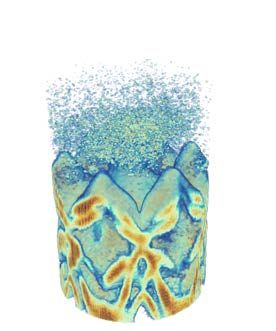
V. Stimper et al.: Multidimensional CLAHE

Algorithm 1 Formulation of the MCLAHE algorithm in
pseudocode. Here, // denotes the integer division operator,
CDF the cumulative distribution function, and map the
intensity mappings applied to the high dimensional pixels
Input: data_in
Parameters: kernel_size (array of integers for all kernel
dimensions), clip_limit (threshold value in [0, 1] for clipping
the local histograms), n_bins (number of bins of the local
histograms)
Output: data_out
  1: pad_len = 2 · kernel_size - 1 + ((shape(data_in) - 1) mod
     kernel_size)
  2: data_hist = symmetric_padding(data_in, [pad_len // 2,
     (pad_len + 1) // 2])
  3: b_list = split data_hist into kernels of size kernel_size
  4: for each b in b_list do
  5:   h = histogram(b, n_bins)
  6:   Redistribute weight in h above clip_limit equally
       across h
  7:   cdf_b = cdf(h)
  8:   map[b] = (cdf_b - min(cdf_b)) / (max(cdf_b) -
       min(cdf_b))
  9: end for
                                                                     FIGURE 2. Illustration of the concepts related to the MCLAHE algorithm
 10: for each neighboring kernel do                                  in 2D. In (a)-(c) the image is equipartitioned into kernels of size (b0 , b1 )
 11:   for each pixel p in data_in do                                bounded by solid black lines. The dotted black lines indicate regions with
 12:      u = map[b in neighboring kernel of p](p)                   pixels having the same nearest-neighbor kernels. Color coding is used to
                                                                     specify the types of border regions, with the areas in green, orange and
 13:      for d = 0 . . . D-1 do                                     magenta having four, three and two nearest-neighbor kernels,
 14:         u = u · (coefficient of the neighboring kernel in       respectively. (a) The original image data in 2D that are divided into
                                                                     kernels. (b) A zoomed-in region of (a). The red square mark in
             dimension d)                                            (b) represents a pixel under consideration and the four blue square
 15:      end for                                                    marks represent the closest kernel centers next to the red one. The
                                                                     distances between the red pixel and the nearest-neighbor kernel centers
 16:      Assign u to pixel p in data_out                            are labeled as d00 , d01 , d10 , d11 , respectively. (c) The padded image with
 17:    end for                                                      the original image now bounded by solid red lines and the padding
 18: end for                                                         indicated by the hatchings. The padding lengths in 2D are labeled as p00 ,
                                                                     p01 , p10 , p11 in (c) and their values are calculated using Eq. (2).
 19: return data_out

                                                                     the index i, then
Here, the // sign denotes integer division. To keep the local                                 mi (In ) = CDF
                                                                                                         d i (In ),                            (3)
intensity distribution at the border of the image unchanged,
the padding is implemented by mirroring the intensities along        where CDF
                                                                             d i represents the normalized CDF obtained from
the boundaries of the data (symmetric padding). The padding          the clipped histogram of the kernel with the index i. As shown
procedure is described in lines 1–2 in Algorithm 1.                  in Fig. 2(b), the bilinear interpolations for the pixel in con-
                                                                     sideration located at the red square mark are computed using
C. MULTIDIMENSIONAL INTERPOLATION
                                                                     the four nearest-neighbor kernels centered on the blue square
                                                                     mark. The interpolation coefficients, ci , are represented as
To derive a generic expression for the intensity mapping
                                                                     Lagrange polynomials [35], [36] using the kernel size (b0 , b1 )
in arbitrary dimensions, we start with the example in 2D
                                                                     and the distances (d00 , d01 , d10 , d11 ) between the pixel and
CLAHE, where each pixel intensity In (n being the pixel
                                                                     the kernel centers in the two dimensions.
index) is transformed by a bilinear interpolation of the
mapped intensities obtained from the normalized CDF of the                                   (b0 − d00 )(b1 − d10 )
                                                                                      c00 =                          ,             (4)
nearest-neighbor kernels [4], [5]. We introduce the kernel                                            b0 b1
index i = (i0 , i1 ) ∈ {0, 1}2 . The values of 0 and 1 in the                         c01 =
                                                                                             (b0 − d00 )(b1 − d11 )
                                                                                                                     ,             (5)
binary alphabet {0, 1} represent the two sides (i.e. above and                                        b0 b1
below), respectively, in a dimension divided by the pixel in                                 (b0 − d01 )(b1 − d10 )
                                                                                      c10 =                          ,             (6)
consideration. For the 2D case, the index (i0 , i1 ) can take any                                     b0 b1
value of (0, 0), (0, 1), (1, 0) and (1, 1), as shown in Fig. 2(b).                           (b0 − d01 )(b1 − d11 )
Let mi be the intensity mapping obtained from the kernel with                         c11 =                          .             (7)
                                                                                                      b0 b1
165440                                                                                                                              VOLUME 7, 2019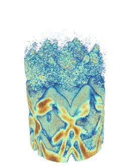
V. Stimper et al.: Multidimensional CLAHE

The transformed intensity Ĩn from In is given by,                          IV. APPLICATIONS
                                                                            We now apply the MCLAHE algorithm to two cases in
Ĩn = c00 m00 (In )+c01 m01 (In )+c10 m10 (In )+c11 m11 (In ). (8)
                                                                            the natural sciences that involve large densely sampled 4D
Eq. (4)-(7) and (8) can be rewritten in a compact form using                (3D+time) data. Each example includes a brief introduction
the kernel index i introduced earlier,                                      of the background knowledge on the type of measurement,
                     Ĩn =
                           X
                                 ci mi (In ),            (9)                the resulting image data features and the motivation for the
                                                                            use of contrast enhancement, followed by discussion and
                               i∈{0,1}2
                                                                            comparison of the outcome using MCLAHE. The perfor-
                               1
                               Y bj − djij                                  mance details are provided at the end of each example.
                        ci =                     .                   (10)
                                          bj
                               j=0
In the 2D case, the term djij takes on the value dji0 or dji1 .             A. PHOTOEMISSION SPECTROSCOPY
The choice of i0 and i1 from the binary alphabet {0, 1} in                  1) BACKGROUND INFORMATION
djij follows that of the kernel index i. The special cases of               In photoemission spectroscopy, the detector registers elec-
transforming the border pixels in the image are naturally                   trons liberated by intense vacuum UV or X-ray pulses from
resolved in our case after data padding (see Section III.B).                a solid state material sample [20]. The measurement is car-
   In D dimensions, the kernel index i = (i0 , i1 , . . . , iD−1 ) ∈        ried out in the so-called 3D momentum space, spanned by
{0, 1}D . Analogous to the two-dimensional case described                   the coordinates (kx , ky , E), in which kx , ky are the electron
before, the intensity mapping of each D-dimensional pixel is                momenta and E the energy. The detected electrons form
now calculated by multilinear interpolation between the 2D                  patterns carrying information about the anisotropic electronic
nearest-neighbor kernels in all dimensions, mathematically,                 density distribution within the material. The fourth dimension
Ĩn = c00...0 m00...0 (In ) + c00...1 m00...1 (In )                         in time-resolved photoemission spectroscopy represent the
                                                                            waiting time in observation by photoemission since the elec-
          + . . . + c11...0 m11...0 (In ) + c11...1 m11...1 (In ).   (11)
                                                                            tronic system is subject to an external perturbation (i.e. light
Similarly, Eq. (11) and the corresponding expressions for the               excitation). The negative time frames represent the observa-
interpolation coefficients can be written in a compact form                 tions taking place before the light excitation. In the image
using the kernel index i as                                                 data acquired in photoemission spectroscopy, the inhomo-
                            X                                               geneous intensity modulation from the experimental geom-
                    Ĩn =        ci mi (In ),           (12)
                                                                            etry, light-matter interaction [37] and scattering background
                               i∈{0,1}D
                                                                            creates contrast variations within and between the so-called
                               D−1
                               Y     bj − djij                              energy bands, which manifest themselves as intercrossing
                        ci =                     .                   (13)   curves (in 2D) or surfaces (in 3D) blurred by convolution
                                          bj
                               j=0                                          with the instrument response function and further affected
The formalism introduced for the 2D case in Eq. (8)-(10)                    by other factors such as the sample quality and the dimen-
generalizes to arbitrary dimensions with only an update to                  sionality of the electronic system, etc [20]. Visualization and
the kernel index i. In Algorithm 1, the calculation of intensity            demarcation of the band-like image features are of great
mappings through interpolation is described in lines 12–15.                 importance for understanding the momentum-space elec-
                                                                            tronic distribution and dynamics in multidimensional pho-
D. ADAPTIVE HISTOGRAM RANGE                                                 toemission spectroscopy [17]. However, in addition to the
In the original formulation of CLAHE in 2D [4], [5], the local              physical limitations on the contrast inhomogeneities listed
histogram ranges for all kernels are the same, which works                  before, the intensity difference between the lower bands
well when the kernels contain intensities in a similarly wide               (or valence bands) and the upper bands (or conduction bands)
range. Tuning of the trade-off between noise amplification                  on the energy scale is on the order of 100 or higher and
and the signal enhancement is then achieved through selec-                  varies by the materials under study and light excitation condi-
tion of the kernel size and the clip limit [31]. However,                   tions. To improve the image contrast in multiple dimensions,
if different patches of the image data contain local features               we applied MCLAHE to a 4D (3D+time) dataset measured
within vastly different but narrow intensity ranges, they may               for the time- and momentum-resolved electronic dynamics of
accumulate in very few histogram bins with values specified                 tungsten diselenide (WSe2 ), a semiconducting material with
globally. Accounting for the disparity in CLAHE will require                highly dispersing electronic bands [38]. The 4D data were
a high clip limit and therefore comes with the price of noise               obtained from an existing experimental setup [39] and pro-
amplification in many parts of the data. This problem may be                cessed using a custom pipeline [40], [41] from detected single
ameliorated by adaptively choosing the local histogram range                photoelectron events. For comparison of contrast enhance-
to lie within the minimum and maximum of the intensity                      ment, we applied both 3D and 4D CLAHE to the 4D pho-
values of the kernel, while keeping the number of bins the                  toemission spectroscopy data. In the case of 3D CLAHE,
same for all kernels. An example use case of the AHR is                     the algorithm was applied to the 3D data at each time frame
presented in Section IV.A.                                                  separately.

VOLUME 7, 2019                                                                                                                       165441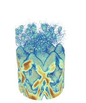
V. Stimper et al.: Multidimensional CLAHE

         FIGURE 3. Applications of MCLAHE to 4D (3D+time) photoemission spectroscopy data featuring the temporal evolution of the electronic
         band structure of the semiconductor WSe2 during and after optical excitation (see Section IV.A). Four time steps in the 4D time series are
         selected for visualization, including the raw data in (a)-(d), the 3D CLAHE-processed data in (e)-(h) and the 4D CLAHE-processed data in
         (i)-(l). The adaptive histogram range (AHR) setting in the MCLAHE algorithm was included in the data processing. All 3D-rendered images
         in (a)-(l) share the same color scaling shown in (l). The integrated dynamics in (n)-(o) over the region specified by the box in (m) in
         the over the 3D momentum space show that the 4D CLAHE amplifies less noise while better preserves the dynamical timescale than the
         3D CLAHE, in comparison with the original data.

165442                                                                                                                                       VOLUME 7, 2019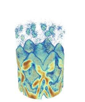
V. Stimper et al.: Multidimensional CLAHE

TABLE 1. Contrast metrics for photoemission spectroscopy data.    argument that 4D CLAHE is superior to its 3D counterpart
                                                                  overall in content-preserving contrast enhancement.

                                                                  3) PROCESSING DETAILS
                                                                  The raw 4D photoemission spectroscopy data have a size
                                                                  of 180 × 180 × 300 × 80 in the (kx , ky , E, t) dimensions.
                                                                  They were first denoised using a Gaussian filter with standard
                                                                  deviations of 0.7, 0.9 and 1.3 along the momenta, energy and
                                                                  time dimensions, respectively. In the applications of both 3D
                                                                  and 4D CLAHE, we set a clip limit of 0.02 and assigned
                                                                  256 grey-level bins to the local histograms. The kernel size
                                                                  for 4D CLAHE was (30, 30, 15, 20) and for 3D CLAHE
2) RESULTS AND DISCUSSION
                                                                  the same kernel size for the first three dimensions, or (kx ,
Stills from the raw data and the results are compared
                                                                  ky , E), was used. Both GHR and AHR settings were tested
in Fig. 3, along with the contrast metrics computed and
                                                                  for comparison. The processing ran on a server with 64 Intel
listed in Table 1. The supplementary files include videos
                                                                  Xeon CPUs at 2.3 GHz and 254GB RAM. The total runtime,
1-3 and video 4 for comparing unprocessed and processed
                                                                  including memory copy operations, for processing the whole
data rendered in 2D slices and in 3D, respectively. As shown
                                                                  dataset with 4D CLAHE was about 5.3 mins. In addition,
in Fig. 3(a)-(d), the original photoemission spectroscopy data
                                                                  we benchmarked the performance of 4D CLAHE on the GPU
are visualized poorly on an energy scale covering both the
                                                                  (NVIDIA GeForce GTX 1070, 8GB RAM) of the server
valence (lower) and conduction (upper) bands. The situation
                                                                  using the first 25 time frames of the dataset. The total runtime
is much improved in the MCLAHE-processed data with AHR
                                                                  was 34 s with the GPU versus 104 s without the GPU,
setting shown in Fig. 3(e)-(l), where the population dynamics
                                                                  representing a 3.1-fold speed-up.
in the conduction band of WSe2 [42], [43] and the broadening
of the valence bands are sufficiently visible to be placed on
the same colorscale, allowing to identify and correlate fine      B. FLUORESCENCE MICROSCOPY
features of the momentum-space dynamics. The improve-             1) BACKGROUND INFORMATION
ment in contrast is also reflected quantitatively in Table 1      In 4D fluorescence microscopy, the measurements are carried
in the drastic changes in standard deviation [32] between         out in the Cartesian coordinates of the laboratory frame,
the unadjusted (smoothed) and processed data. On the other        or (x, y, z), with the fourth dimension representing the obser-
hand, the GHR setting of MCLAHE cannot visualize the              vation time t since fertilization. In practice, the photophysics
upper bands well (see comparisons in supplementary videos         of the fluorophores [44], the autofluorescence background
1-3) because the regions in the lower and upper bands con-        [21] from the labeled and unlabeled parts of the sample
tain drastically different intensity features. Next, we com-      and the detection method, such as the attenuation effect
pare performance between 3D and 4D CLAHE under the                from scanning measurements at different depths or nonuni-
AHR setting. The decrease in MSE (0.1121 → 0.1050)                form illumination of fluorophores [45], pose limits on the
or, equivalently, the increase in PSNR (147.98 → 148.26)          achievable image contrast in the experiment. The image fea-
shown in Table 1 indicates that 4D CLAHE is more suited           tures in fluorescence microscopy data often include sparsely
here because a smaller MSE implies closer resemblance to          labeled cells and cellular components such as the nuclei,
the original data [31]. Furthermore, visual inspection of the     membranes, dendritic structures, and other organelles. The
results in Fig. 3(e)-(l) and in supplementary videos 1-4 finds    limited contrast may render the downstream data annotation
less severe noise enhancement when applying 4D CLAHE to           tasks, such as segmentation, tracking and lineage tracing [46],
the whole dataset than 3D CLAHE to each time frame.               [47], challenging. Therefore, a digital contrast enhancement
   To quantify the influence of contrast enhancement on the       method is potentially useful to improve the visibility of the
dynamical features in the data, we calculated the integrated      cells and their corresponding dynamics. We demonstrate the
intensity in the conduction band of the data in all three cases   use of MCLAHE for this purpose on a publicly available
and the results are summarized in Fig. 3(m)-(o). The standard     4D (3D+time) fluorescence microscopy dataset [22] of the
score in Fig. 3(o) is used to compare the integrated signals      embryo development of ascidian (Phallusia mammillata),
in a scale-independent fashion. The dynamics represented          or sea squirt. The organism is stained and imaged in toto
in the intensity changes are better preserved in 4D than 3D       to reveal its development from a gastrula to tailbud forma-
CLAHE-treated data and the former are less influenced by          tion with cellular resolution [22]. During embryo develop-
the boundary artifacts in the beginning and at the end of         ment, the fluorescence contrast exhibits time dependence
the time delay range. The artefactual delays created by 3D        due to cellular processes such as division and differentia-
CLAHE in the onset and recovery of changes, around t1 and         tion. We use the data from one fluorescence label channel
t3 in Fig. 3(o), respectively, are shown even clearer in the      containing the nuclei and process through the MCLAHE
supplementary videos 1-4. These observations reinforce the        pipeline.

VOLUME 7, 2019                                                                                                             165443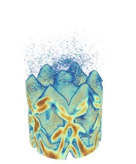
V. Stimper et al.: Multidimensional CLAHE
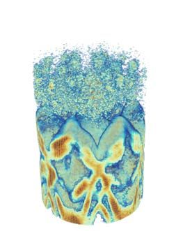
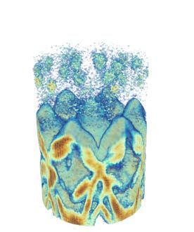
FIGURE 4. Applications of MCLAHE to 4D (3D+time) fluorescence microscopy data of the embryo development of ascidian (Phallusia
mammillata), or sea squirt. Four time frames (hpf = hours post fertilization) in the 4D time series are visualized here for comparison,
including the raw data in (a)-(d), the 3D CLAHE-processed data in (e)-(h) and the 4D CLAHE-processed data in (i)-(l). All images in (a)-(l)
are rendered in 3D with the same axes, orientation and the same color scaling as in (l). Both 3D and 4D CLAHE-processed data show
drastic improvement in the image contrast, while the results from 4D CLAHE better preserves the dynamical intensity features from the
cellular processes.
TABLE 2. Contrast metrics for fluorescence microscopy data. intensities are similar throughout the organism. Additionally,
the dynamic range of the data is limited (see the following
Processing details) and the changes in fluorescence during
development are relatively small. The initial high Shannon
entropy of the raw data in Table 2 is due to its high back-
ground noise, which is reduced after smoothing, as indicated
2) RESULTS AND DISCUSSION by the sharp drop in the entropy while the standard devia-
The results are compared with the original data on the tion shows relative consistency. Then, the use of MCLAHE
same colorscale in Fig. 4 and the corresponding contrast increases the entropy again, together with the large changes
metrics are shown in Table 2. The supplementary files in other metrics, this time due to the contrast enhancement.
include video 5 and video 6 for comparing the unprocessed Similarly to the previous example, the 4D CLAHE outper-
and processed data in a 2D slice and in 3D, respectively. forms its 3D counterpart overall because of the lower MSE
As shown in Fig. 4(a)-(d), the intensities in the raw fluores- or, equivalently, the higher PSNR of the 4D results, indicating
cence microscopy data are distributed very unevenly in the a higher similarity to the raw data. In other contrast metrics
colorscale. The MCLAHE-processed 4D time series show such as the standard deviation and the Shannon entropy,
significant improvement in the visibility of the cells against the 4D and 3D results have very close values, indicating
the background signal (e.g. autofluorescence, detector dark the complexity of judging image contrast by a single metric.
counts, etc). This is reflected in the surge in contrast repre- Visualization of the dynamics in Fig. 4(e)-(l) also shows that
sented by standard deviation as shown in Table 2. In con- the 4D CLAHE-processed data preserve more of the fluores-
trast to the previous example, the AHR option in MCLAHE cence intensity change than its 3D counterpart, while main-
was not used in processing the embryo development dataset taining a high cell-to-background contrast. More complete
because the cellular feature sizes and their fluorescence comparisons of unprocessed and processed data are presented
165444 VOLUME 7, 2019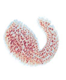
V. Stimper et al.: Multidimensional CLAHE

in the supplementary videos 5-6. The contrast-enhanced            procedures, such as those in [8], [54], [55], which will provide
embryo development data potentially allow better tracking of      a wider choice of algorithms for multidimensional image
cellular lineage and dynamics [47], [48], which are challeng-     processing and comprehensive comparison of the algorithm
ing due to sparse fluorescent labeling.                           performance on data with various characteristics.

3) PROCESSING DETAILS                                             VI. CONCLUSION
The raw 4D fluorescence microscopy data have a size               We present a flexible and efficient generalization of the
of 512 × 512 × 109 × 144 in the (x, y, z, t) dimensions.          CLAHE algorithm to arbitrary dimensions for contrast
They were first denoised by a median filter with a kernel size    enhancement of complex multidimensional imaging and
of (2, 2, 2, 1). In the application of 4D CLAHE, the kernel       spectroscopy datasets. Our algorithm, the multidimensional
size of choice was (20, 20, 10, 25) and the same kernel size      CLAHE, improves upon previous lower-dimensional equiv-
in the first three dimensions were used for 3D CLAHE to           alents [4], [5], [19] by its unified treatment of image bound-
enable direct comparison. For both MCLAHE procedures,             aries, flexible kernels size selection, adaptive histogram range
the clip limit was set at 0.25 and the number of histogram        determination. Its parallelized implementation in Tensorflow
bins at 256. The intensities in the raw data were given as        allows computational acceleration with multiple CPUs and
8 bit unsigned integers resulting in only 256 possible values.    GPUs. We demonstrate the effectiveness of multidimensional
Hence, only the GHR setting was used because the AHR              CLAHE by visual analysis and contrast quantification in
setting would result in bins smaller than the resolution of the   case studies drawn from different measurement techniques,
data. Processing with MCLAHE ran on the same server as            namely, 4D (3D+time) photoemission spectroscopy and 4D
for the photoemission spectroscopy data (see Section IV.A).       fluorescence microscopy, with the capabilities of producing
The total runtime for processing the whole dataset using only     densely sampled high dimensional data. In the example appli-
CPUs was about 26 mins. Similar to the photoemission case         cations, our algorithm greatly improves and balances the visi-
study, the speed-up by GPU usage was tracked. The total           bility of multidimensional image features in diverse intensity
runtime for processing the first 8 time frames of the dataset     ranges and neighborhood conditions. We further show that
was 32 s on the GPU versus 85 s only on CPUs, representing        the best overall performance in each case comes from the
a 2.7-fold speed-up.                                              simultaneous application of multidimensional CLAHE to all
                                                                  data dimensions, in line with the observation for applying
V. PERSPECTIVES                                                   CLAHE to 3D data [19]. In addition, we provide the imple-
While we have presented the applications of the MCLAHE            mentation of multidimensional CLAHE in an open-source
algorithm to real-world datasets of up to multiple gigabytes      codebase to assist its reuse and integration into existing image
in size, its current major performance limitation is in the       analysis pipelines in various domains of natural sciences and
memory usage, since the data needs to be loaded entirely          engineering.
into the RAM (of CPUs or GPUs), which may be challeng-
ing for very large imaging and spectroscopy datasets on the       ACKNOWLEDGMENTS
multi-terabyte scale that are becoming widely available [13].     The authors thank S. Schülke, G. Schnapka at the GNZ
Future improvements on the algorithm implementation may           (Gemeinsames Netzwerkzentrum) in Berlin and M. Rampp
include distributed handling of chunked datasets to enable        at the MPCDF (Max Planck Computing and Data Facility)
operation on limited hardware resource by loading each            in Garching for computing supports. The authors also thank
time only a subset of the data. In addition, the number of        S. Dong and S. Beaulieu for performing the photoemission
nearest-neighbor kernels currently required for intensity map-    spectroscopy measurement on a tungsten diselenide sample
ping interpolation increases exponentially with the dimen-        at the Fritz Haber Institute. V. Stimper thanks U. Gerland for
sionality D of the data (see Section III.C). For datasets with    administrative support.
D < 10, this may not pose an outstanding issue, but for even
higher-dimensional datasets, new strategies may be devel-         REFERENCES
oped for approximate interpolation of selected neighboring         [1] B. A. Olshausen and D. J. Field, ‘‘Vision and the coding of natu-
kernels to alleviate the exponential scaling.                          ral images: The human brain may hold the secrets to the best image-
   On the other hand, the applications of MCLAHE are not               compression algorithms,’’ Amer. Sci., vol. 88, no. 3, p. 238, 2000. [Online].
                                                                       Available: http://www.americanscientist.org/issues/feature/2000/3/vision-
limited by the examples given in this work but are open                and-the-coding-of-natural-images
to other types of data. It is especially beneficial to the         [2] W. K. Pratt, Digital Image Processing, 4th ed. Hoboken, NJ, USA: Wiley,
preprocessing of high dimensional data with dense sam-                 2007.
pling produced by various fast volumetric spectroscopic and        [3] E. L. Hall, ‘‘Almost uniform distributions for computer image enhance-
                                                                       ment,’’ IEEE Trans. Comput., vols. C-23, no. 2, pp. 207–208, Feb. 1974.
imaging techniques [49]–[53] for improving the performance         [4] S. M. Pizer, E. P. Amburn, J. D. Austin, R. Cromartie, A. Geselowitz,
of feature annotation and extraction tasks.                            T. Greer, B. ter Haar Romeny, J. B. Zimmerman, and K. Zuiderveld,
   Furthermore, the call for extension of the image processing         ‘‘Adaptive histogram equalization and its variations,’’ Comput.
                                                                       Vis., Graph., Image Process., vol. 39, no. 3, pp. 355–368, 1987.
toolkits in 2D and 3D to higher-dimensional imaging datasets           [Online]. Available: http://www.sciencedirect.com/science/article/pii/
also motivates the dimensional extension of more recent CE             S0734189X8780186X

VOLUME 7, 2019                                                                                                                             165445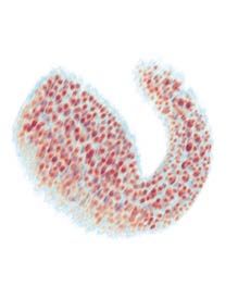
V. Stimper et al.: Multidimensional CLAHE

 [5] K. Zuiderveld, ‘‘Contrast limited adaptive histogram equalization,’’           [24] V. Stimper and R. P. Xian. (2019). Multidimensional Contrast Limited
     in Graphics Gems. Amsterdam, The Netherlands: Elsevier, 1994,                       Adaptive Histogram Equalization. [Online]. Available: https://github.com/
     pp. 474–485. [Online]. Available: https://linkinghub.elsevier.com/retrieve/         VincentStimper/mclahe
     pii/B9780123361561500616                                                       [25] P. K. Sinha, Image Acquisition and Preprocessing for Machine Vision
 [6] M. S. Hitam, E. A. Awalludin, W. N. J. H. W. Yussof, and Z. Bachok,                 Systems. Bellingham, WA, USA: SPIE, 2012.
     ‘‘Mixture contrast limited adaptive histogram equalization for under-          [26] D. J. Ketcham, ‘‘Real-time image enhancement techniques,’’ Proc. SPIE,
     water image enhancement,’’ in Proc. Int. Conf. Comput. Appl. Tech-                  vol. 74, pp. 120–125, Jul. 1976, doi: 10.1117/12.954708.
     nol. (ICCAT), Jan. 2013, pp. 1–5. [Online]. Available: http://ieeexplore.      [27] R. Hummel, ‘‘Image enhancement by histogram transformation,’’
     ieee.org/document/6522017/                                                          Comput. Graph. Image Process., vol. 6, no. 2, pp. 184–195, 1977.
 [7] E. D. Pisano, S. Zong, B. M. Hemminger, M. DeLuca, R. E. Johnston,                  [Online]. Available: http://www.sciencedirect.com/science/article/pii/
     K. Muller, M. P. Braeuning, and S. M. Pizer, ‘‘Contrast limited adaptive            S0146664X77800117
     histogram equalization image processing to improve the detection of sim-       [28] R. Dale-Jones and T. Tjahjadi, ‘‘A study and modification of the
     ulated spiculations in dense mammograms,’’ J. Digit. Imag., vol. 11, no. 4,         local histogram equalization algorithm,’’ Pattern Recognit., vol. 26,
     p. 193, Nov. 1998, doi: 10.1007/BF03178082.                                         no. 9, pp. 1373–1381, Sep. 1993. [Online]. Available: https://linkinghub.
 [8] J. Dabass, S. Arora, R. Vig, and M. Hanmandlu, ‘‘Mammogram                          elsevier.com/retrieve/pii/003132039390143K
     image enhancement using entropy and CLAHE based intuitionistic                 [29] J. A. Stark, ‘‘Adaptive image contrast enhancement using generaliza-
     fuzzy method,’’ in Proc. 6th Int. Conf. Signal Process. Integr. Netw.               tions of histogram equalization,’’ IEEE Trans. Image Process., vol. 9,
     (SPIN), Mar. 2019, pp. 24–29. [Online]. Available: https://ieeexplore.ieee.         no. 5, pp. 889–896, May 2000. [Online]. Available: http://ieeexplore.
     org/document/8711696/                                                               ieee.org/document/841534/
 [9] M. Z. Yildiz, O. F. Boyraz, E. Guleryuz, A. Akgul, and I. Hussain,             [30] Z. Wang, A. C. Bovik, H. R. Sheikh, and E. P. Simoncelli, ‘‘Image quality
     ‘‘A novel encryption method for dorsal hand vein images on a microcom-              assessment: From error visibility to structural similarity,’’ IEEE Trans.
     puter,’’ IEEE Access, vol. 7, pp. 60850–60867, 2019. [Online]. Available:           Image Process., vol. 13, no. 4, pp. 600–612, Apr. 2004. [Online]. Available:
     https://ieeexplore.ieee.org/document/8705292/                                       http://ieeexplore.ieee.org/document/1284395/
[10] J. Xiao, S. Li, and Q. Xu, ‘‘Video-based evidence analysis and extraction
                                                                                    [31] G. F. C. Campos, S. M. Mastelini, G. J. Aguiar, R. G. Mantovani,
     in digital forensic investigation,’’ IEEE Access, vol. 7, pp. 55432–55442,
                                                                                         L. F. de Melo, and S. Barbon, Jr., ‘‘Machine learning hyperparameter
     2019. [Online]. Available: https://ieeexplore.ieee.org/document/8700194/
                                                                                         selection for contrast limited adaptive histogram Equalization,’’ EURASIP
[11] K. S. Sim, Y. Y. Tan, M. A. Lai, C. P. Tso, and W. K. Lim,
                                                                                         J. Image Video Process., vol. 2019, no. 1, p. 59, Dec. 2019. [Online].
     ‘‘Reducing scanning electron microscope charging by using exponential
                                                                                         Available: https://jivp-eurasipjournals.springeropen.com/articles/10.1186/
     contrast stretching technique on post-processing images,’’ J. Microsc.,
                                                                                         s13640-019-0445-4
     vol. 238, no. 1, pp. 44–56, Apr. 2010. [Online]. Available: http://doi.
                                                                                    [32] E. Peli, ‘‘Contrast in complex images,’’ J. Opt. Soc. Amer. A, Opt.
     wiley.com/10.1111/j.1365-2818.2009.03328.x
                                                                                         Image Sci., vol. 7, no. 10, p. 2032, Oct. 1990. [Online]. Available:
[12] A. J. McCollum and W. F. Clocksin, ‘‘Multidimensional histogram equal-
                                                                                         https://www.osapublishing.org/abstract.cfm?URI=josaa-7-10-2032
     ization and modification,’’ in Proc. 14th Int. Conf. Image Anal. Process.
                                                                                    [33] K. Gu, G. Zhai, W. Lin, and M. Liu, ‘‘The analysis of image con-
     (ICIAP), Sep. 2007, pp. 659–664. [Online]. Available: http://ieeexplore.
                                                                                         trast: From quality assessment to automatic enhancement,’’ IEEE Trans.
     ieee.org/document/4362852/
                                                                                         Cybern., vol. 46, no. 1, pp. 284–297, Jan. 2016. [Online]. Available:
[13] W. Ouyang and C. Zimmer, ‘‘The imaging tsunami: Computational
                                                                                         http://ieeexplore.ieee.org/document/7056527/
     opportunities and challenges,’’ Current Opinion Syst. Biol., vol. 4,
     pp. 105–113, Aug. 2017. [Online]. Available: https://linkinghub.elsevier.      [34] A. Kriete, ‘‘Image quality considerations in computerized 2-D and 3-D
     com/retrieve/pii/S2452310017300537                                                  microscopy,’’ in Multidimensional Microscopy. New York, NY, USA:
[14] P. Pantazis and W. Supatto, ‘‘Advances in whole-embryo imaging: A quan-             Springer, 1994, pp. 209–230. [Online]. Available: http://link.springer.
     titative transition is underway,’’ Nature Rev. Mol. Cell Biol., vol. 15,            com/10.1007/978-1-4613-8366-6_12
     no. 5, pp. 327–339, May 2014. [Online]. Available: http://www.nature.          [35] G. M. Phillips, Interpolation and Approximation by Polynomials (CMS
     com/articles/nrm3786                                                                Books in Mathematics). New York, NY, USA: Springer, 2003. [Online].
[15] L. Gao and L. V. Wang, ‘‘A review of snapshot multidimensional opti-                Available: http://link.springer.com/10.1007/b97417
     cal imaging: Measuring photon tags in parallel,’’ Phys. Rep., vol. 616,        [36] E. Kreyszig, H. Kreyszig, and E. J. Norminton, Advanced Engineering
     pp. 1–37, Feb. 2016. [Online]. Available: https://linkinghub.elsevier.              Mathematics, 10th ed. Hoboken, NJ, USA: Wiley, 2011.
     com/retrieve/pii/S0370157315005025                                             [37] S. Moser, ‘‘An experimentalist’s guide to the matrix element in
[16] O. Ersen, I. Florea, C. Hirlimann, and C. Pham-Huu, ‘‘Exploring nano-               angle resolved photoemission,’’ J. Electron Spectrosc. Rel. Phenomena,
     materials with 3D electron microscopy,’’ Mater. Today, vol. 18, no. 7,              vol. 214, pp. 29–52, Jan. 2017. [Online]. Available: https://linkinghub.
     pp. 395–408, Sep. 2015. [Online]. Available: https://linkinghub.elsevier.           elsevier.com/retrieve/pii/S0368204816301724
     com/retrieve/pii/S1369702115001200                                             [38] J. M. Riley, F. Mazzola, M. Dendzik, M. Michiardi, T. Takayama,
[17] G. Schönhense, K. Medjanik, and H.-J. Elmers, ‘‘Space-, time- and                   L. Bawden, C. Granerød, M. Leandersson, T. Balasubramanian,
     spin-resolved photoemission,’’ J. Electron Spectrosc. Rel. Phenomena,               M. Hoesch, T. K. Kim, H. Takagi, W. Meevasana, P. Hofmann,
     vol. 200, pp. 94–118, Apr. 2015. [Online]. Available: http://linkinghub.            M. S. Bahramy, J. W. Wells, and P. D. C. King, ‘‘Direct observation
     elsevier.com/retrieve/pii/S0368204815001243                                         of spin-polarized bulk bands in an inversion-symmetric semiconductor,’’
[18] J. H. Moore, C. C. Davis, M. A. Coplan, and S. C. Greer, Building Scientific        Nature Phys., vol. 10, no. 11, pp. 835–839, Nov. 2014. [Online]. Available:
     Apparatus, 4th ed. Cambridge, U.K.: Cambridge Univ. Press, 2009.                    http://www.nature.com/articles/nphys3105
[19] P. Amorim, T. Moraes, J. Silva, and H. Pedrini, ‘‘3D adaptive histogram        [39] M. Puppin, Y. Deng, C. W. Nicholson, J. Feldl, N. B. M. Schröter,
     equalization method for medical volumes,’’ in Proc. 13th Int. Joint Conf.           H. Vita, P. S. Kirchmann, C. Monney, L. Rettig, M. Wolf, and
     Comput. Vis., Imag. Comput. Graph. Theory Appl., 2018, pp. 363–370.                 R. Ernstorfer, ‘‘Time- and angle-resolved photoemission spectroscopy of
     [Online].         Available:       http://www.scitepress.org/DigitalLibrary/        solids in the extreme ultraviolet at 500 kHz repetition rate,’’ Rev. Sci.
     Link.aspx?doi=10.5220/0006615303630370                                              Instrum., vol. 90, no. 2, Feb. 2019, Art. no. 023104. [Online]. Available:
[20] S. Hüfner, Photoelectron Spectroscopy: Principles and Applications,                 http://aip.scitation.org/doi/10.1063/1.5081938
     3rd ed. Berlin, Germany: Springer, 2003.                                       [40] R. P. Xian, L. Rettig, and R. Ernstorfer, ‘‘Symmetry-guided non-
[21] U. Kubitscheck, Ed., Fluorescence Microscopy: From Principles to Bio-               rigid registration: The case for distortion correction in multidimensional
     logical Applications, 2nd ed. Weinheim, Germany: Wiley, 2017. [Online].             photoemission spectroscopy,’’ Ultramicroscopy, vol. 202, pp. 133–139,
     Available: http://doi.wiley.com/10.1002/9783527687732                               Jul. 2019. [Online]. Available: https://linkinghub.elsevier.com/retrieve/pii/
[22] E. Faure et al., ‘‘A workflow to process 3D+time microscopy images                  S0304399118303474
     of developing organisms and reconstruct their cell lineage,’’ Nature           [41] R. P. Xian, Y. Acremann, S. Y. Agustsson, M. Dendzik, K. Bühlmann,
     Commun., vol. 7, no. 1, Apr. 2016, Art. no. 8674. [Online]. Available:              D. Curcio, D. Kutnyakhov, F. Pressacco, M. Heber, S. Dong, J. Demsar,
     http://www.nature.com/articles/ncomms9674                                           W. Wurth, P. Hofmann, M. Wolf, L. Rettig, and R. Ernstorfer, ‘‘An open-
[23] M. Abadi et al., ‘‘TensorFlow: Large-scale machine learning on hetero-              source, distributed workflow for band mapping data in multidimensional
     geneous distributed systems,’’ Mar. 2016, arXiv:1603.04467. [Online].               photoemission spectroscopy,’’ Sep. 2019, arXiv:1909.07714. [Online].
     Available: https://arxiv.org/abs/1603.04467                                         Available: https://arxiv.org/abs/1909.07714

165446                                                                                                                                                VOLUME 7, 2019
V. Stimper et al.: Multidimensional CLAHE
[42] R. Bertoni, C. W. Nicholson, L. Waldecker, H. Hübener, C. Monney, STEFAN BAUER received the M.Sc. degree in
U. De Giovannini, M. Puppin, M. Hoesch, E. Springate, R. T. Chapman, mathematics and the Ph.D. degree in computer
C. Cacho, M. Wolf, A. Rubio, and R. Ernstorfer, ‘‘Generation and evo- science from ETH Zurich, Zurich, Switzerland,
lution of spin-, valley-, and layer-polarized excited carriers in inversion- in 2014 and 2018, respectively. During his studies,
symmetric WSe2 ,’’ Phys. Rev. Lett., vol. 117, no. 27, Dec. 2016, he held scholarships from the Swiss and German
Art. no. 277201. [Online]. Available: https://link.aps.org/doi/10.1103/ National Merit Foundation. He was awarded the
PhysRevLett.117.277201 ETH medal for outstanding doctoral thesis. He is
[43] M. Puppin, ‘‘Time- and angle-resolved photoemission spectroscopy
currently a Research Group Leader with the Max
on bidimensional semiconductors with a 500 kHz extreme ultravio-
Planck Institute for Intelligent Systems, Tübingen,
let light source,’’ Ph.D. dissertation, Dept. Phys., Free Univ. Berlin,
Berlin, Germany, Sep. 2017. [Online]. Available: https://refubium.fu- Germany. His current research focuses on causal
berlin.de/handle/fub188/23006?show=full inference, reinforcement learning, representation learning, and robotics.
[44] B. Valeur and M. N. Berberan-Santos, Molecular Fluorescence: Principles Recently, he and his team received the Best Paper Award at the International
and Applications, 2nd ed. Hoboken, NJ, USA: Wiley, 2013. [Online]. Conference on Machine Learning (ICML), in 2019.
Available: https://www.wiley.com/enus/Molecular+Fluorescence%
3A+Principles+and+Applications%2C+2nd+Editionp-9783527328376
[45] J. C. Waters, ‘‘Accuracy and precision in quantitative fluorescence
microscopy,’’ J. Cell Biol., vol. 185, no. 7, pp. 1135–1148, RALPH ERNSTORFER received the Diploma
Jun. 2009. [Online]. Available: http://www.jcb.org/lookup/doi/10.1083/ degree in physics from the Technical University
jcb.200903097 of Munich, Munich, Germany, in 1999, and the
[46] T. A. Nketia, H. Sailem, G. Rohde, R. Machiraju, and J. Rittscher, ‘‘Anal- Ph.D. degree in physics from the Free University
ysis of live cell images: Methods, tools and opportunities,’’ Methods, of Berlin, Berlin, Germany, in 2004. After post-
vol. 115, pp. 65–79, Feb. 2017. [Online]. Available: https://linkinghub.
doctoral research at the University of Toronto in
elsevier.com/retrieve/pii/S104620231730083X
Canada and at the Max Planck Institute for Quan-
[47] K. Kretzschmar and F. M. Watt, ‘‘Lineage tracing,’’ Cell, vol. 148,
nos. 1–2, pp. 33–45, Jan. 2012. [Online]. Available: https://linkinghub. tum Optics in Germany, he became the Leader
elsevier.com/retrieve/pii/S0092867412000037 of the Max Planck Research Group ‘‘Structural
[48] F. Amat, W. Lemon, D. P. Mossing, K. McDole, Y. Wan, K. Branson, and Electronic Surface Dynamics,’’ in 2010, at the
E. W. Myers, and P. J. Keller, ‘‘Fast, accurate reconstruction of cell Fritz Haber Institute of the Max Planck Society, Berlin, Germany. His
lineages from large-scale fluorescence microscopy data,’’ Nature Meth- group currently investigates the structural and electronic dynamics of
ods, vol. 11, no. 9, pp. 951–958, Sep. 2014. [Online]. Available: low-dimensional semiconductors and heterostructures using a combina-
http://www.nature.com/articles/nmeth.3036 tion of time-resolved photoemission spectroscopy and electron diffraction.
[49] D. J. Flannigan and A. H. Zewail, ‘‘4D electron microscopy: Principles In 2016, he received the Consolidator Grant FLATLAND from the European
and applications,’’ Accounts Chem. Res., vol. 45, no. 10, pp. 1828–1839, Research Council.
Oct. 2012. [Online]. Available: http://pubs.acs.org/doi/10.1021/ar3001684
[50] G. Lu and B. Fei, ‘‘Medical hyperspectral imaging: A review,’’ J. Biomed.
Opt., vol. 19, no. 1, Jan. 2014, Art. no. 010901. [Online]. Available:
http://biomedicaloptics.spiedigitallibrary.org/article.aspx?doi=10.1117/1.
BERNHARD SCHÖLKOPF received the Ph.D.
JBO.19.1.010901
[51] W. Jahr, B. Schmid, C. Schmied, F. O. Fahrbach, and J. Huisken,
degree in computer science from Technical Uni-
‘‘Hyperspectral light sheet microscopy,’’ Nature Commun., vol. 6, versity of Berlin, in 1997. His thesis on support
no. 1, Nov. 2015, Art. no. 7990. [Online]. Available: http://www.nature. vector learning received the annual dissertation
com/articles/ncomms8990 prize of the German Association for Computer
[52] A. Özbek, X. L. Deán-Ben, and D. Razansky, ‘‘Optoacoustic imag- Science (GI). He has conducted research at AT&T
ing at kilohertz volumetric frame rates,’’ Optica, vol. 5, no. 7, Bell Labs, GMD FIRST, Berlin, the Australian
p. 857, Jul. 2018. [Online]. Available: https://www.osapublishing.org/ National University, Canberra, and Microsoft
abstract.cfm?URI=optica-5-7-857 Research Cambridge, U.K. In July 2001, he was
[53] M. K. Miller and R. G. Forbes, Atom-Probe Tomography. Boston, appointed as a Scientific Member of the Max
MA, USA: Springer, 2014. [Online]. Available: http://link.springer. Planck Society. He currently leads the Department of Empirical Infer-
com/10.1007/978-1-4899-7430-3 ence, Max Planck Institute for Intelligent Systems, Tübingen, Germany.
[54] A. Mehrish, A. V. Subramanyam, and S. Emmanuel, ‘‘Joint spatial and He received numerous awards, including, recently, the prestigious Gottfried
discrete cosine transform domain-based counter forensics for adaptive Wilhelm Leibniz Prize of the German Research Foundation (DFG), in 2018,
contrast enhancement,’’ IEEE Access, vol. 7, pp. 27183–27195, 2019.
and the Körber Prize, in 2019.
[Online]. Available: https://ieeexplore.ieee.org/document/8658078/
[55] S. F. Tan and N. A. M. Isa, ‘‘Exposure based multi-histogram equal-
ization contrast enhancement for non-uniform illumination images,’’
IEEE Access, vol. 7, pp. 70842–70861, 2019. [Online]. Available:
https://ieeexplore.ieee.org/document/8721128/ RUI PATRICK XIAN received the M.Sc. degree in
physics from the University of Waterloo, Waterloo,
Ontario, Canada, in 2012, and the Ph.D. degree in
VINCENT STIMPER received the B.Sc. degree in physics from the University of Hamburg and the
physics from the Technical University of Munich, Max Planck Institute for the Structure and Dynam-
Munich, Germany, in 2017. After a summer intern- ics of Matter, Hamburg, Germany, in 2016. From
ship in bioinformatics at the Ontario Institute 2017 to 2019, he was a Postdoctoral Fellow with
for Cancer Research, Toronto, Ontario, Canada, the Fritz Haber Institute of the Max Planck Society,
he resumed his studies in physics in Munich at the Berlin, Germany. Since summer 2019, he holds a
Technical University of Munich. Since fall 2018, Postdoctoral Fellow position with the Department
he has been doing research for his M.Sc. degree of Neurobiology, Northwestern University, Evanston, Illinois, USA. He has
with the Department of Empirical Inference, Max worked on a variety of projects, including optical imaging, quantum comput-
Planck Institute for Intelligent Systems, Tübingen, ing, magnetic resonance, ultrafast condensed matter spectroscopy, electron
Germany. His current focus is on applying machine learning techniques to diffraction and crystallography, photoemission spectroscopy, neuroimaging,
materials informatics and to infer physical knowledge from massive amounts image processing, and metadata management.
of materials characterization data.
VOLUME 7, 2019 165447You can also read