Forecasting basketball players' performance using sparse functional data - UV
←
→
Page content transcription
If your browser does not render page correctly, please read the page content below
Forecasting basketball players’ performance using sparse
                    functional data
                            G. Vinué(1) , I. Epifanio(2)
(1) Department of Statistics and O.R., University of Valencia, 46100 Burjassot, Spain.
   (2) Dept. Matemàtiques and Institut de Matemàtiques i Aplicacions de Castelló.
          Campus del Riu Sec. Universitat Jaume I, 12071 Castelló, Spain.

Abstract
Statistics and analytic methods are becoming increasingly important in bas-
ketball. In particular, predicting players’ performance using past observa-
tions is a considerable challenge. The purpose of this study is to forecast
the future behavior of basketball players. The available data are sparse func-
tional data, which are very common in sports. So far, however, no fore-
casting method designed for sparse functional data has been used in sports.
A methodology based on two methods to handle sparse and irregular data,
together with the analogous method and functional archetypoid analysis is
proposed. Results in comparison with traditional methods show that our
approach is competitive and additionally provides prediction intervals. The
methodology can also be used in other sports when sparse longitudinal data
are available.
Keywords: Forecasting, Functional data analysis, Archetypal analysis,
Functional sparse data, Basketball

1. Introduction
   The statistical analysis of sports is a fast-growing field. In particular,
sports forecasting is a strongly expanding field. Proof of this is the increas-
ing number of forecasting methods developed covering several sports and
sportive topics [37]. Certainly, in professional sports, getting any notion in

    Email address: guillermo.vinue@uv.es, epifanio@mat.uji.es (G. Vinué(1) , I.
Epifanio(2) )

Preprint submitted to Statistical Analysis and Data Mining                May 9, 2019
advance about the future performance of players can have important conse-
quences on the roster composition in terms of renewing or buying players,
or in terms of establishing levels of remuneration in function of that perfor-
mance, for instance. One of the sports that has been revolutionized by data
analytics is basketball. Basketball analytics started to attract attention with
the publications by [24] and [17]. More recently, other papers and books have
been released [22, 34, 32]. Technological advances have made it possible to
collect more data than ever about what is happening on the field, requiring
new methods of analysis. There is currently a need for innovative methods
that exploit the full potential of the data and that make it possible to gener-
ate additional value for athletes and technical staff. Here too, one of the main
challenges is to use past performance to predict future performance [32]. To
address this open question, some forecasting methods have been developed.
Following [19, Chapter 1.4], two main approaches can be distinguished based
on the type of data used: time-series forecasting and cross-sectional forecast-
ing. On the one hand, forecasting using data collected over time describes the
likely outcome of the time series in the immediate future, based on knowledge
of recent outcomes. On the other hand, cross-sectional forecasting methods
use data collected at a single point in time. The goal here is to predict a
target variable using some explanatory variables which are related to it.
Two well elaborated methods can be found using historical time data:
(i) College Prospect Rating (CPR), which is a score assigned to college bas-
ketball players that attempts to estimate their NBA potential [32, 33]; (ii)
Career-Arc Regression Model Estimator with Local Optimization (CARMELO),
which, for a player of interest, identifies similar players throughout NBA his-
tory and uses their careers to forecast the future player’s activity [35].
Regarding cross-sectional models, a Weibull-Gamma with covariates tim-
ing model is proposed in [18] to predict the points scored by players over time.
In this case, the time variable is years playing in NBA. Another interesting
approach is presented in [30], where correlations and regression models are
computed to figure out which foreign players will be successful in the NBA,
by using their previous statistics in international competitions.
In addition to the effort of predicting individual performance, there have
also been other approaches focusing on teams and other features of the game.
Some models using simulation have been developed to forecast the outcome
of a basketball match [38, 43]. A comparison between predictions based on
NCAAB and NBA match data is discussed in [47]. A dynamic paired com-
parison model is described in [3] for the results of matches in two basketball
2and football tournaments. Furthermore, in [4] a process model is used with
player tracking data for predicting possession outcomes.
We wish to consider a new perspective by using Functional Data Analysis
(FDA) in sports. FDA is a relatively new branch of Statistics that analyses
data drawn from continuous underlying processes, often time, i.e. a whole
function is a datum. Let us assume that n smooth functions, x1 (t), ..., xn (t),
are observed, with the i-th function measured at ti1 ,..., tini points. In our
study, xi (t) represents the metric value of player i for a certain age t. An
important point we would like to emphasize here is that the time component
of the FDA approach we are considering will represent players’ ages. As such,
in this paper we propose different models for aging curves, which is a well-
recognized and important topic within the more general area of forecasting
player performance. As mentioned in [35], the most important attribute of
all, in terms of determining a player’s future career trajectory, is his/her age.
The goals of FDA coincide with those of any other branch of Statis-
tics, and the classical summaryPn statistics can be also defined, such as the
−1
meanPfunction x̄(t) = n i=1 xi (t), the variance function varX (t) = (n −
1)−1 Pni=1 (xi (t) − x̄(t))2 and the covariance function covX (th , tl ) = (n −
1)−1 ni=1 (xi (th ) − x̄(th ))(xi (tl ) − x̄(tl )). An excellent overview of FDA is
found in [28], while methodologies for studying functional data nonparamet-
rically are found in [15]. [29] introduces related software and [27] presents
some interesting applications in different fields. Other recent applications
include [9] and [23]. In all these problems, a continuous function lies behind
these data even though functions are sampled discretely at certain points.
The FDA framework is highly flexible since the sampling time points do not
have to be equally spaced and both the argument values and their cardinality
can vary across cases. When functions are observed over a relatively sparse
set of points, we have sparse functional data. An excellent survey on sparsely
sampled functions is provided by [21].
As regards the forecast of functional time series, there is a body of re-
search, such as [31, 2, 20], where functions are measured over a fine grid
of points. However, only a few works deal with the problem of forecasting
sparse functional data [11]. Notice that when functions are observed over a
dense grid of time points, it is possible to fit a separate function for each case
using any reasonable basis. Nevertheless, in the sparse case, this approach
fails and the information from all functions must be used to fit each function.
This is because each individual has been observed at different time points.
Therefore, any fixed grid that is formed will contain many missing observa-
3tions for each curve. A very good explanation of this issue can be found in
[21].
Sports data are sparse and irregular. They are sparse because most play-
ers do not have a very long career in the same league. And they are irregular
because each player’s career lasts for a different length of time. Despite
the fact that time series data or movement trajectories are very common in
sports, FDA has been mostly used in sport biomechanics or medicine [14, 16].
To the best of our knowledge, there are only two references about sports ana-
lytics using FDA. In [44], FDA was introduced for the study of players’ aging
curves and both hypothesis testing and exploratory analysis were performed.
[41] extended archetypoid analysis (ADA) for sparse functional data (see also
[42, 13]), showing the potential of FDA in sports analytics. In particular, in
[41, Section 5.2] it was demonstrated that advanced analysis with FDA re-
veals patterns in the players’ trajectories over the years that could not be
discovered if data were simply aggregated (averaged, for example). We take
advantage of this fact and continue the work done in [41, Section 5.2] with a
view to predict how players will evolve.
In this paper, we propose a methodology to predict player’s performances
using sparse functional data. Two metrics will be analyzed: Box Plus/Minus
(BPM)1 and Win Shares (WS)2 . Analysis using BPM will allow us to estab-
lish a plausible comparison with CARMELO, while analysis with another
variable such as WS will allow us to evaluate differences in career arcs. To
that end, we will focus on two existing methods designed to handle sparse and
irregular data: (i) Regularized Optimization for Prediction and Estimation
with Sparse data (ROPES), originally developed by Alexander Dokumentov
and Rob Hyndman [11, 10]; (ii) Principal components Analysis through Con-
ditional Expectation (PACE), originally developed by Fang Yao, Hans-Georg
Müller and Jane-Lin Wang [45].
Our methodology will also involve using the method of analogues based
on functional archetypoid analysis (FADA), which will allow us to refine
predictions for the players of interest and to achieve a more reliable forecast,
in line with the expectations of basketball analysts. We will apply them to a
very comprehensive database of NBA players. Results will be obtained using
the R software [25].
1
https://www.basketball-reference.com/about/bpm.html
2
https://www.basketball-reference.com/about/ws.html
4As noted earlier, forecasting future performance is also very relevant to
other sports (see for instance [1]). We would like to emphasize that our
methodology can also be used in other sports when sparse longitudinal data
are available. Data and R code (including a web application created with
the R package shiny [5]) to reproduce the results can be freely accessed at
https://www.uv.es/vivigui/software. The rest of the paper is organized
as follows: Section 2 reviews ROPES, PACE, ADA and FADA. Section 3 will
be concerned with the data and input variables used. Section 4 presents three
analyses: (i) A validation study is carried out to choose an optimal blend
of tuning parameters which ROPES depends on; (ii) ROPES and PACE are
compared with each other and with standard benchmarks; (iii) The reliabil-
ity of ROPES predictions for current players using the method of analogues
with FADA is shown. A comparison with CARMELO results is also pro-
vided and the implications of the archetypoid coefficients is discussed. The
paper ends with some conclusions in Section 5. An appendix shows how this
methodology can also be proposed for forecasting international players.
2. Methodology
2.1. ROPES
The method ROPES (Regularized Optimization for Prediction and Es-
timation with Sparse data), proposed by Alexander Dokumentov and Rob
Hyndman [11, 10], solves problems involving decomposing, smoothing and
forecasting two-dimensional sparse data. In practical terms, where the aim
is to interpolate and extrapolate the sparse longitudinal data, made up of n
observations, and presented over the time dimension with m time points, the
following optimization problem is solved:
{(U, V )} = argmin ||W (Y − U V T )||2 + ||U ||2 + ||DIFF2 (m, λ2 )V ||2 +
U,V
||DIFF1 (m, λ1 )V ||2 + ||DIFF0 (m, λ0 )V ||2
(1)
where:
• Y is an n × m matrix.
• U is an n × k matrix of “scores” (“coefficients”), k = min(n, m).
5• V is an m × k matrix of “features” (“shapes”).
• ||.|| is the Frobenius norm.
• is the element-wise matrix multiplication.
• W is an n × m “masking matrix” of weights.
• λ0 , λ1 and λ2 are smoothing parameters.
and where DIFFi (m, λ) represents the discrete i times derivative operator
multiplied by the scalar λ. In particular, DIFF0 (m, λ) is the identity matrix
m × m multiplied by the scalar λ; DIFF1 (m, λ) is the matrix (m − 1) × m,
with −λ values in the main diagonal, λ values in the following upper diagonal
and 0 otherwise; DIFF2 (m, λ) is the matrix (m − 2) × m, with λ values in
the main diagonal, −2λ values in the following upper diagonal, λ values in
the following upper diagonal, and 0 otherwise.
ROPES is equivalent to maximum likelihood estimation with partially
observed data, which allows the calculation of confidence and prediction in-
tervals. They are estimated using a Monte-Carlo style method. The original
two sources [11, 10] should be referred to for all the specific details.
2.2. PACE
Functional Principal Components Analysis (FPCA) is a common tool to
reduce the dimension of data when the observations are random curves. The
usual computational methods for FPCA based on function discretization or
basis function expansions are inefficient when data with only a few repeated
and sufficiently irregularly spaced measurements per subject are available.
As a quick reminder, when functions are measured over a fine grid of time
points, a separate function for each individual can be used. In the sparse
case, however, the information from all functions must be used to fit each
function.
A version of FPCA, in which the FPC scores are framed as conditional
expectations, was developed by Fang Yao, Hans-Georg Müller and Jane-Lin
Wang to overcome this issue [45]. This method was referred to as Principal
components Analysis through Conditional Expectation (PACE) for sparse
and irregular longitudinal data. In practice, the prediction for the trajectory
Xi (t) for the ith subject, using the first p φq eigenfunctions, is:
6p
X
X̂ip (t) = µ̂ + ξˆiq φˆq (t) (2)
q=1
where µ̂ is the estimate of the mean function E(X(t)) = µ(t) and ξiq are
the FPC scores. PACE and its implementation in the R library fdapace
([7]) use local smoothing techniques to estimate the mean and covariance
functions of the trajectories, specifically a local weighted bilinear smoother
is used for estimating the covariance. Generalized Cross Validation is used
for bandwidth choice, which is the default method for the FPCA function
in the R library fdapace (default parameters are considered; for example,
10 folds and a Gaussian kernel are used). The number of components p is
determined using the Fraction-of-Variance-Explained threshold (0.9999 by
default) computed during the SVD of the fitted covariance function.
The eigenfunctions φ̂q (t) and the number p are estimated with the training
set, and they are used in the estimation of the scores for the test set. This is
the procedure we will follow in Section 4.2. With the scores and the estimated
eigenfunctions, we obtain an approximation of the trajectories and they can
be used to predict unobserved portions of the functions. [45] also explains
the construction of asymptotic pointwise confidence intervals for individual
trajectories and asymptotic simultaneous confidence bands.
2.3. ADA
Archetypoid analysis (ADA) was presented in [42] and is an extension
of archetypal analysis defined by [6] (see [8, 26] for other derived method-
ologies). In ADA, archetypes correspond to real observations (the so-called
archetypoids). Let X be an n × p matrix of real numbers representing a
multivariate data set with n observations and p variables. For a given g, the
objective of ADA is to find a g × p matrix Z that characterizes the archety-
pal patterns in the data. In ADA, the optimization problem is formulated
as follows:
n g n g n
X X X X X
2
RSS = kxi − αij zj k = kxi − αij βjl xl k2 , (3)
i=1 j=1 i=1 j=1 l=1
under the constraints
g
X
1) αij = 1 with αij ≥ 0 and i = 1, . . . , n and
j=1
7n
X
2) βjl = 1 with βjl ∈ {0, 1} and j = 1, . . . , g i.e., βjl = 1 for one and
l=1
only one l and βjl = 0 otherwise.
Archetypoids are computed with the R package Anthropometry [40].
2.3.1. ADA for sparse data with FDA
ADA was defined for functions in [13], where it was shown that functional
archetypoids can be obtained as in the multivariate case if the functions are
expressed in an orthonormal basis, simply by applying ADA to the basis
coefficients. When functions are measured over some sparse points, we have
sparse functional data.
The basic idea of functional archetypoid analysis (FADA) is as follows.
Based on the Karhunen-Loève expansion, the functions are approximated as
in Eq. 2. Because the eigenfunctions are orthonormal, to obtain FADA we
can apply ADA to the n × p matrix X, with the scores (the coefficients in
the Karhunen-Loève basis).
3. Data
We have used the R package ballr [12] to obtain the total advanced
statistics for each NBA player from the 1973-1974 season to the latest sea-
son, 2017-2018, including the player’s age on February 1st of that season
(the convention in https://www.basketball-reference.com/ is to provide
players’ age at the start of February 1st of every season). From the total set
of statistics, we have focused on Box Plus/Minus (BPM) and Win Shares
(WS).
BPM is a box score-based variable for estimating basketball players’ qual-
ity and contribution to the team. It takes into account both the players’
statistics and the team’s overall performance. The final value enables us
to evaluate the player’s performance relative to the league average. BPM
is a per-100-possession statistic and its scale is as follows: 0 is the league
average, +5 means that the player has contributed 5 more points than an
average player over 100 possessions, −2 is replacement level, and −5 is very
bad. Replacement level players are those who replace a roster spot for short-
term contracts, so they are not normal members of a team’s rotation. We
have chosen BPM because it was created to only use the information that is
available historically. This means that BPM only takes into account those
8stats that have always been available in the box-scores. It does not consider
new stats derived from play-by-play data or from tracking data. According
to the website where BPM is explained 3 , “it is possible to create a better stat
than BPM for measuring players, but difficult to make a better one that can
also be used historically”, which fits perfectly with the goal of our method.
BPM is available from the 1973-1974 season.
We have chosen a second metric, which is also widely used: Win Shares
(WS). It also has the advantage of taking the surrounding team into ac-
count. In particular, WS is a player statistic that distributes the team’s
success among the team players. It is calculated using player, team and
league statistics. The sum of all the players’ WS in a given team will be
approximately equal to that team’s total wins for the season. A player with
negative WS means that the player took away wins that the teammates had
generated.
The reason for analyzing two variables is to investigate differences in
career arcs for different aspects of skill. This allows us to highlight the power
of our approach and could be of interest to basketball fans/analysts. Any
other statistic can be chosen.
We have removed the observations with fewer than five games played.
They were related to very extreme BPM values, such as −86.7 for Gheorghe
Muresan in 1998-19994 or −49.3 for Mindaugas Kuzminskas in 2017-20185 .
Fig. 1 illustrates the type of data we are working with. It shows the obser-
vations of certain players, whose values are represented as connected points.
Players’ ages will represent the time points to be used by our methodology.
The initial range of ages in the database went from 18 to 44 years old. How-
ever, there were only a few measurements between ages 41 and 44, related to
a few long-lasting players, so we have removed them. The age range finally
considered is from 18 to 40 years old, i.e., there are 23 time points. In total
there are 3075 players.
3
https://www.basketball-reference.com/about/bpm.html
4
https://www.basketball-reference.com/players/m/muresgh01.html#all_
advanced
5
https://www.basketball-reference.com/players/k/kuzmimi01.html#all_
advanced
9BPM Win Shares
20
10
Arvydas Sabonis
15
Drazen Petrovic
Joel Embiid
5 10
Kareem Abdul−Jabbar
LeBron James
5
0
20 25 30 35 40 20 25 30 35 40
Age (years)
Figure 1: BPM and Win Shares values for some players present in the database, at their
corresponding ages (colors in the online version). We have chosen these players because of
two reasons: Firstly, we wanted to represent the values of well-known players. Sabonis and
Petrovic are two of the best international players of all time. Abdul-Jabbar and James are
two of the best players in history. Embiid is one of the most promising players nowadays.
Secondly, we wanted to fill the entire range of ages, both with short and long careers.
4. Results
In Section 4.1 a validation study is proposed to choose an appropriate
combination of ROPES tuning parameters, which is crucial for good predic-
tive activity. Section 4.2 contains a comparison analysis between ROPES,
PACE and two benchmark methods. Section 4.3 discusses the implications
of the archetypoid coefficients. Section 4.4 specifies the type of projections
obtained. Section 4.5 presents an interactive web application.
4.1. Selection of parameters
ROPES depends on three tuning parameters (λ2 , λ1 , λ0 ), which have to
be chosen to guarantee that the model itself returns predictions with enough
accuracy. We evaluate the precision of the model’s prediction in terms of the
mean squared error (MSE). MSE measures the average of the squares of the
differences between the predicted values ŷ and the true values y across all
individual estimates i, as shown in Eq. (4).
10n n
1X 1X 2
M SE = (ŷi − yi )2 = e (4)
n i=1 n i=1 i
We adopt MSE since ROPES uses it to measure the error term. In order
to select the parameters, we proceed as follows: our goal will be to predict
the BPM in the 2017-2018 season, for the players who played at least in one
season before the 2017-2018 season and who also played in the 2017-2018
season itself. The justification for doing this is related to sporting reasons.
In sports, when coaches and managers are building their rosters, it is highly
important for them to have a basic idea about how players will perform
during the following season. Of course, they would also like to know the
players’ performance in the long term, but most rosters are built according
to the most immediate season. This would allow them to decide whether
the current roster should remain the same for the next season or whether
some players should be replaced. This procedure makes sense because we
will consider the previous performance of all the players selected, but we are
only interested in predicting their BPM for the next season, by taking into
account each player’s data and the information about the other players. This
procedure is more computationally efficient than the leave-one-out approach.
From the 3075 players, there are 385 who played in the 2017-2018 sea-
son and at least another season before that. Firstly, we split our data into
a training+validation set (TrVaSet) with 2690 (3075 − 385) players and a
test set with the 385 aforementioned players. No test set player belongs to
TrVaSet. We will select the optimal combination of λ’s with TrVaSet. To
do this, we have carried out an exhaustive 10-fold cross-validation for each
parameter combination j. Inside each fold i, we use 60% observations as the
training set and the remaining observations as the validation set. The mean
squared error, MSEij , is then computed on the observations of the validation
set. Finally, we obtain the MSEj for every j by averaging across folds. For
the validation players, their BPM value is replaced by NA in the Y matrix.
In the W masking matrix the 1 value is then replaced by 0.
Let’s define the parameter combinations. The first step is to optimize the
parameter λ2 , setting λ1 = 0 and λ0 = 10. The parameter λ2 takes values
in a sequence from 0 to 1000 in increments of 100. In this way, the first
blend is (λ2 = 0, λ1 = 0, λ0 = 10), the second is (λ2 = 100, λ1 = 0, λ0 = 10)
and so on. We are looking for smooth curves, so we place more emphasis
on λ2 because it is related to the second derivative and this derivative is
11strongly related to the smoothness of the curve. This is justified because
if the second derivative is a smooth curve, both the first derivative and the
original function will also be smooth. From the definition of derivative, it
directly follows that if a function has a first derivative at any point, then it
does not have a sharp bend (v-shape) at that point (the same can be said of
the second derivative with respect to the first derivative). See for example
[28, Section 5.2.2] for further insights. The opposite is not always true.
Fig. 2 shows the averaged MSE across folds for every combination when
only λ2 is moving. The smallest MSE was for the combination with λ2 = 900.
1.987
2.0
1.878 1.872 1.877 1.872 1.864 1.856 1.857 1.856 1.853 1.854
1.5
minimum_mse
MSE
1.0 No
Yes
0.5
0.0
0
10
10
10
10
10
10
10
10
10
_1
10
0_
0_
0_
0_
0_
0_
0_
0_
0_
_0
0_
0_
0_
0_
0_
0_
0_
0_
0_
0_
00
0_
10
20
30
40
50
60
70
80
90
10
Figure 2: Averaged MSE across folds for every combination of lambdas when λ2 is moving
and λ0 , λ1 are fixed. The combination for the smallest MSE is highlighted in green (colors
in the online version).
Once the optimal λ2 has been found, we then adjust λ1 and λ0 as well.
Both λ0 and λ1 take values in a sequence from 0 to 10 in increments of 5. Fig.
3 shows the averaged MSE across folds for every combination when both λ0
and λ1 are moving. The smallest MSE was for the combination (λ2 = 900,
λ1 = 10, λ0 = 10).
122.176
2.093
2.04
2.0
1.896 1.902 1.896
1.853 1.852 1.85
1.5
minimum_mse
MSE
No
1.0
Yes
0.5
0.0
0
_0
_5
10
10
0
0
5
5
_1
0_
5_
0_
5_
10
10
0_
5_
10
0_
0_
0_
0_
0_
0_
0_
0_
0_
90
90
90
90
90
90
90
90
90
Figure 3: Averaged MSE across folds for every combination of lambdas when λ2 is fixed
and λ0 , λ1 are moving. The combination for the smallest MSE is highlighted in green
(colors in the online version).
The grid search procedure is chosen since it is a traditional way of per-
forming hyperparameter optimization and can return results in a reason-
able amount of time. This second point was particularly important because
ROPES is computationally expensive. However, we would like to emphasize
that we are not arguing that the grid search is the most efficient approach.
There might be other more efficient alternatives than the grid search. We
aim to investigate them as part of our future work.
4.2. Comparison with other methods
In order to evaluate the usefulness of ROPES and PACE, we carry out a
comparison with each other and with two benchmark methods, such as the
average method and the naı̈ve method. In the average method, the forecast
of the next value is the mean of the previous values. In the naı̈ve option, the
forecast is the value of the last observation. They are two common simple
alternatives to more advanced techniques [19, Section 2.3].
In order to check the performance of all the methods, we have applied
them to the test set of 385 players. Table 1 reports an extract of the results.
It contains the following information for all players in the 2017-2018 season:
(i) their age; (ii) their actual BPM value; (iii) the predictions with ROPES
13Table 1: Actual and predicted BPM values for the 2017-2018 season with ROPES, PACE,
the average method and the naı̈ve method, for the test set of players who played during
the 2017-2018 season and at least one season before. The difference between actual and
predicted values and MSE are also provided. MSE is highlighted in bold. Extract of the
results.
ROPES (900,10,10) PACE Average Naı̈ve
Player Age BPM BPMpr (BPMpr − BPM)2 BPMpr (BPMpr − BPM)2 BPMpr (BPMpr − BPM)2 BPMpr (BPMpr − BPM)2
Aaron Brooks 33 -4.3 -4.14 0.03 -3.32 0.96 -2.21 4.37 -4.6 0.09
... ... ... ... ... ... ... ... ... ... ...
Josh Richardson 24 1.4 0.66 0.55 0.56 0.71 0.40 1.00 0.2 1.44
... ... ... ... ... ... ... ... ... ... ...
Zaza Pachulia 33 0.8 1.00 0.04 0.54 0.07 -0.75 2.40 2.7 3.61
Mean (MSE) -0.92 -0.61 6.73 -0.87 3.24 -1.15 7.59 -0.92 7.11
Sd 3.31 3.01 16.28 2.35 7.6 2.72 15.41 3.22 16.53
Mean ± Sd (2.39,4.23) (2.4, 3.62) (1.48,3.22) (-3.87,1.57) (-4.14,2.3)
(using the optimal λ combination), PACE and the simple methods; (iv) the
squared difference between predictions and actual values (BPMpr − BPM)2 ;
(v) the resulting total MSE (highlighted in bold). PACE obtains the smallest
MSE, followed by ROPES. It is interesting to note that the mean BPM
obtained with the naı̈ve method is practically the same as the actual one
(both rounded to −0.92). This result is most probably because over- and
under-predictions cancel each other out.
Fig. 4 displays the boxplots for the actual BPM values together with the
BPM predictions for each method in different intervals.
[6,11)
[1,6)
actual
BPM observed
average
[−4,1) naive
pace
ropes
[−9,−4)
[−14,−9)
−10 0 10
BPM predicted
Figure 4: Boxplots for the actual BPM values together with the BPM predictions for each
method in different intervals.
14The intervals [−14, −9) and [−9, −4) refer to players with a very bad
performance (according to the BPM scale). We see in both cases that the
predictions are far away from the true values. All the methods give a con-
servative forecast for such extreme values. PACE is the method that pro-
vides the closest results in these two intervals. ROPES is close to PACE
in [−9, −4). In the interval [−4, 1), the four methods show similar values
with respect to the actual ones. In the interval [1, 6), ROPES gives the most
similar predictions with respect to the actual ones. In the interval [6, 11),
again ROPES and PACE give the most accurate predictions. Remarkably,
the naı̈ve method shows outliers in all the intervals. Fig. 4 is showing that
PACE and ROPES tend to overestimate bad players and underestimate good
ones. This can very helpful for team managers in their search for future stars
(this additional interpretation was suggested by one of the referees).
Overall, PACE is the method that performs best. ROPES is able to beat
the simple benchmark methods, showing an improvement with respect to
them. The main drawback of the current PACE implementation is the lack
of prediction intervals. The main goal of this paper is to draw attention to
the added value of using an FDA approach to forecast players’ performance,
which has not been done so far. Therefore, even though PACE should give
somewhat more accurate predictions than ROPES, in next Section we will use
ROPES to forecast future players’ activity because it does provide prediction
intervals. Prediction intervals are very helpful and important because they
express how much uncertainty is associated with the forecast.
4.3. Implications of the archetypoid coefficients
We have analyzed a total of 8 players from different teams, namely Devin
Booker, Clint Capela, Joel Embiid, Nikola Jokic, Tyus Jones, Zach LaVine,
Donovan Mitchell and Jayson Tatum. They are representing several career
status. Embiid, Jokic, Mitchell and Tatum are already established figures
(especially Embiid and Jokic). Booker and Capela are a step below the
super stars but they are also very good players. Something similar could
be said about Tyus Jones, who is constantly improving his skills. Finally,
LaVine is an offensive specialist.
In a first attempt to compute predictions using all the players of the data
set, we realized that the ROPES method had some pull towards the mean
of the entire sample (like the other methods discussed in Section 4.2 but not
as strong as them). This gave unrealistic performance predictions for both
15the best and most promising players. Therefore, in order to refine predic-
tions, it is much more suitable to use the so-called “method of analogues”.
The idea is to find players related to the one of interest and then use their
documented activity to obtain the predictions. We know how other players
already performed, so we can use their information to gain an approximate
idea about the future performances of others. The method of analogues has
been used for years in fields such as climatology [46] and epidemiology [39].
Recently, an R package has been released that contains analogue methods for
palaeoecology [36]. The CARMELO method is also based on this scheme.
In order to find related players, we use archetypoid analysis (ADA, see
[42] for theoretical details). ADA searches for extreme observations (the so-
called archetypoids) to describe the frontiers of the data. In this technique,
the BPM (and WS) function of a player is approximated by a mixture of
archetypoids, which are themselves functions of boundary players (outstand-
ing -positive or negative- performers). Archetypoids are specific players and
the α coefficients represent how much each archetypoid contributes to the
approximation of each individual. The most comparable archetypoid should
be the one corresponding to the largest value of the α coefficients for the
player of interest.
We choose the number of archetypoids for each metric following the
screeplot explained by [42]. Five are selected for BPM and four for WS.
The archetypoids for the BPM metric are (their career BPM shown in
brackets): Devin Gray (−8.4), Darryl Dawkins (−2.52), Diamond Stone
(−24.1), Eddy Curry (−6.5) and LeBron James (9.21).
LeBron James is the representative of super star players. He is one of the
best players in history. This is in line with the expected results since James
has achieved the highest BPM values.
Darryl Dawkins represents the replacement level players (as a reminder,
−2 is replacement level). Dawkins had a long NBA career. He was selected
with the fifth pick in the 1975 NBA draft and played for 14 seasons, where
he averaged double figures in scoring in nine of them. He lead the league in
fouls committed in three seasons. In his case, his performance does not fit
exactly with the replacement level description, but his average BPM does.
Eddy Curry, Devin Gray and Diamond Stone are representatives of play-
ers with a short-term career or with overall poor performance. Eddy Curry
was selected fourth overall in the 2001 NBA draft and had a long NBA ca-
reer. He led the NBA in field goal percentage in the 2002-2003 season but
he did not really meet the expectations that his talent was indicating. Devin
16Gray had an irrelevant NBA career, playing a total of 27 games in two NBA
seasons. Diamond Stone only played seven games in the NBA. From the
basketball point of view, Devin Gray and Diamond Stone are related to the
“bad” archetypical player profile. Both players played very little in the NBA.
However, from the mathematical point of view, they are not exactly repre-
senting the same profile, since Devin Gray has a BPM of -8.4, while Diamond
Stone has a BPM of -24.1 (the third worst BPM value in our database, the
range of BPM values goes from -31.5 to 21). Therefore, Stone is representing
even a much more extreme bad pattern than Gray. We acknowledge that
the five archetypoids computed for BPM are not exactly representing all the
players’ typologies available in the database. In some cases, a greater number
of archetypoids is needed to capture other players’ profiles. Even though we
have determined the optimal number of archetypoids with the screeplot, in a
real situation it would be up to the analyst to decide how many representative
cases to consider.
Regarding the WS metric, the archetypoids are (their career WS shown
in brackets): Steve Burtt (0), Ben Wallace (5.84), Otis Birdsong (4.03) and
LeBron James (14.6). Again, as expected, James is the representative of
super star players. The fact that James is selected as the “best” archetypoid
in both metrics is indicating how he can excel in many aspects of the game.
Otis Birdsong and Ben Wallace represent very good players. Otis Bird-
song played twelve NBA seasons and appeared in four NBA All-Star Games.
He was selected with the second pick of the 1977 NBA draft. Ben Wallace was
very good at grabbing rebounds and blocking opponent shots. He won the
NBA Defensive Player of the Year Award four times and won a championship
with the Pistons in 2004.
Steve Burtt represents ordinary players. He played 101 games in four
NBA seasons between 1984-1985 and 1992-1993.
Table 2 shows the α values for the 8 players selected for the BPM and
WS archetypoids.
17Table 2: Similarity of the 8 players selected to the BPM and WS archetypoids according
to the α coefficients.
BPM Archetypoids
Player D. Gray D. Dawkins D. Stone E. Curry L. James
D. Booker 0.32 0.12 0.07 0.13 0.36
C. Capela 0.00 0.08 0.33 0.10 0.49
J. Embiid 0.23 0.15 0.00 0.13 0.49
N. Jokic 0.06 0.19 0.00 0.07 0.68
T. Jones 0.31 0.14 0.07 0.12 0.36
Z. LaVine 0.39 0.15 0.05 0.11 0.30
D. Mitchell 0.37 0.12 0.00 0.12 0.39
J. Tatum 0.42 0.06 0.00 0.09 0.43
WS Archetypoids
Player S. Burtt B. Wallace O. Birdsong L. James
D. Booker 0.70 0.12 0.08 0.10
C. Capela 0.00 0.14 0.76 0.10
J. Embiid 0.42 0.18 0.29 0.11
N. Jokic 0.19 0.03 0.35 0.43
T. Jones 0.58 0.12 0.24 0.06
Z. LaVine 0.77 0.10 0.07 0.06
D. Mitchell 0.59 0.08 0.12 0.21
J. Tatum 0.59 0.06 0.00 0.35
As mentioned before, in ADA each datum is expressed as a mixture of
actual observations (archetypoids). In particular, the α coefficients of each
player are of great utility because they allow us to determine the compo-
sition of each player according to the archetypoid players, and to establish
a clustering of similar players [41]. A discussion of the implications of the
resulting archetypoid coefficients is given next. The BPM composition of
Embiid is as follows. Embiid’s profile matches 49% of James’, 23% of Gray’s,
15% of Dawkins’ and 13% of Curry’s, so this is reflecting the fact that Em-
biid is on his way to become a super star like James is, but he still has some
room of improvement. Regarding the WS composition, Embiid’s profile is
42% explained by Burtt’s, 29% by Birdsong’s, 18% by Wallace’s and 11%
by James’. In this case, the Embiid’s room for development is even more
evident. The archetypoid coefficients for Jokic are quite impressive. His
highest α is with James in both variables. His BPM profile matches 68%
of James’ BPM profile (the highest similarity to James in this analysis by
far) and his WS profile matches 43% of James’ WS profile (only Tatum has
a close value) and 35% of Birdsong’s. This high similarity with respect to
James implies that Jokic’s performance is already very good. Capela is an-
other player worth highlighting. His highest BPM coefficient is also with
James, though his profile still matches 33% of Stones’, which indicates some
18shortcomings in his performance. Regarding his WS composition, his profile
matches 76% of Birdsong’s, 14% of Wallace’s and 10% of James’, which indi-
cates a remarkable team productivity. On the other hand, the BPM profiles
for Booker, Jones, Tatum and Mitchell are as close to James’ as to Gray’s.
In terms of James’ coefficient, it is very difficult to approach his excellence,
so we shouldn’t expect Booker, Jones, Tatum and Mitchell to achieve such
an incredible level. However, the Gray’s coefficient is also indicating that
their performance is not very far away from an average player yet, so they
still need to make further efforts to display a difference from competitors.
Their WS profiles reaffirm this claim. Finally, the LaVine’s BPM and WS
profiles are most similar to Gray’s and Burtt’s profiles, respectively, so he is
not showing an outstanding performance at all.
4.4. Projections of future performance with ROPES and the method of ana-
logues. Comparison with CARMELO
In order to select the cluster of analogous players, we first choose the
archetypoid with the highest α. As an illustration, Embiid’s greatest simi-
larity for BPM is with James. Then, the group of BPM similar players to
Embiid is made up of James, together with the other players whose largest α
coefficient is also for James and who have an α value greater than Embiid’s
α. We will use this cluster to forecast the Embiid’s future career arc. Current
stars such as Chris Paul or Kevin Durant and stars of previous seasons such
as Michael Jordan or Charles Barkley belong to this set. Likewise for WS.
The ROPES algorithm (with the lambda combination obtained in the
validation study) is used to obtain p-forecasting intervals, where p = 0.05 is
the selected significance level. We will discuss the ROPES predictions with
the ones that the CARMELO 2018-2019 version provides6 . CARMELO is
a basketball forecasting system released in the 2015-2016 season. Successive
versions present some improvements [35]. To the best of our knowledge, it
is the only publicly available projection system to compare our approach
against. For each player of interest, CARMELO computes the similarity
scores between that player and all historical players. To that end, it uses a
number of statistics and players’ attributes and a version of a nearest neigh-
bor algorithm. The Wins Above Replacement (WAR) metric is computed
for all historical players with a positive similarity score. The forecast is given
6
https://projects.fivethirtyeight.com/carmelo/
19by averaging these WAR values.
WAR reflects a combination of a player’s projected playing time and his
projected productivity while on the court. Productivity is measured by a
blend of two-thirds Real Plus-Minus (RPM) and one-third Box Plus/Minus
(BPM). BPM was solely used to make the 2016-2017 forecasts, but the combi-
nation of RPM and BPM is used for the 2018-2019 forecasts (as in 2015-2016
and 2017-2018). According to the developers of CARMELO, the RPM/BPM
blend seems to outperform BPM alone. The RPM statistic quantifies how
much a player hurts or helps his/her team when (s)he is on the court. There
has been some controversy regarding the validity of RPM, since the com-
putations are not detailed 7 . In fact, the CARMELO methodology cannot
be replicated either. In addition, for seasons before 2000-01, no RPM is
available and CARMELO uses BPM only. The final point that needs to be
made is that RPM is not available in our database. Therefore, we would like
to draw the reader’s attention to the fact that our results are not directly
equivalent to those of CARMELO, since the target variable is not exactly
the same. However, both approaches should be complementary.
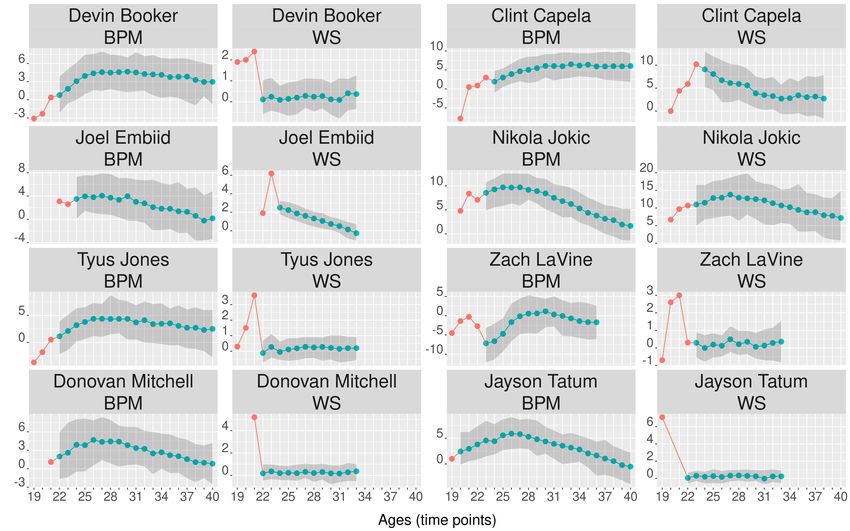
Fig.5 shows the ROPES forecast obtained for the 8 players selected. In
addition, for the sake of a convenient comparison with CARMELO, Fig. 6
shows the screenshots of the CARMELO curves for the same 8 players.
In Fig.5 we see that the predictions for Jokic show that his BPM and WS
are expected to increase in the next three seasons and will remain quite high
for several seasons (though they will go down from age 28). His lower and
upper predictions are also high values. The width of the prediction intervals
is constant over seasons. In general, the width of the intervals remain quite
stable for most players. As a referee rightly mentioned, the intervals show
several possible scenarios for some players, going from high to low values, so
there is some uncertainty related to the point predictions. The CARMELO
forecast for Jokic indicates some decrease in his performance, but still keeping
high numbers (Fig. 6d). The width of the CARMELO intervals fluctuates,
the uncertainty in the ’20 season is bigger than in the ’19 and ’21 seasons.
The BPM-ROPES forecast for Embiid shows that he will improve his BPM
in the two coming seasons and then his performance will slowly decline.
Regarding WS, it indicates a constant decrease over time. CARMELO also
indicates that Embiid’s performance will increase within two seasons and
7
https://www.boxscoregeeks.com/articles/rpm-and-a-problem-with-advanced-stats
20Figure 5: BPM and WS predictions for Devin Booker, Clint Capela, Joel Embiid, Nikola
Jokic, Tyus Jones, Zach LaVine, Donovan Mitchell and Jayson Tatum using only the set
of analogue players. Past values are in red and predictions are in green (colors in the
online version). The shaded area indicates the limits of the prediction intervals.
21(a) Devin Booker (b) Clint Capela
(c) Joel Embiid (d) Nikola Jokic
(e) Tyus Jones (f) Zach LaVine
(g) Donovan Mitchell (h) Jayson Tatum
Figure 6: CARMELO curves for Devin Booker, Clint Capela, Joel Embiid, Nikola Jokic,
Tyus Jones, Zach LaVine, Donovan Mitchell and Jayson Tatum.
22then his values will decrease (the intervals move between narrow and wide
intervals, Fig. 6c). The BPM-ROPES forecast for Capela shows a constant
increase in the coming years, keeping good values for many seasons. On the
other hand, his WS values will constantly decrease. In this case, the intervals
are widening over the years (especially in the BPM facet). The CARMELO
forecast for Capela is a bit more conservative. Its prediction intervals are a
bit wider in the ’20 and ’21 seasons than in the ’19 season and then narrow a
bit again (Fig. 6b). The BPM-ROPES forecast for Devin Booker and Tyus
Jones are somewhat similar to Capela’s. However, their WS-ROPES forecast
is a flat arc around 0. The CARMELO predictions for these two players
show a certain increase in their activity (Fig. 6a and Fig. 6e). The width
of the prediction interval for Booker remains quite constant. For Jones the
width interval fluctuates between some wide and narrow ranges. The BPM-
ROPES prediction for Donovan Mitchell and Jayson Tatum are similar to
Jokic’s, though their values are not so outstanding. Their WS prediction is a
flat arc around 0. The CARMELO predictions for Mitchell and Tatum also
show a constant increase in their activity (Fig. 6g and Fig. 6h). In both
cases, the width of the prediction interval also fluctuate between some wide
and narrow ranges. Finally, the BPM-ROPES forecast for LaVine shows a
constant increase but keeping negative numbers, especially for the next four
years. His WS prediction moves around 0. CARMELO also suggests an
ordinary and flat performance in the coming seasons (Fig. 6f). It is worth
mentioning that some of the WS predictions stop at age 33 because this is
the last age for which the set of analogous players shows values. For Mitchell,
Booker and Tatum, WS-ROPES has been too conservative. Higher values
would have been a bit more realistic, since everything seems to indicate
that these three players will become very good players in the near future.
Another aspect that demands a careful examination of the results is that the
WS prediction for Booker climbs to about 0.5 in the last two years. These
are some pitfalls worth highlighting for end-users of this methodology.
As a final point, it is important to remember that statistical models are
not completely reliable for long-term forecasts, because the assumption that
the future looks similar to the past slowly breaks down the further we go
into the future. So the predictions should be constantly updated as new
data becomes available.
234.5. Web application
Additionally, an interactive web application available at https://www.
uv.es/vivigui/AppPredPerf.html allows the user to represent the BPM
and WS forecasting plots for every player in the 2017-2018 season under the
age of 24 (154 players in total). A link to the CARMELO forecast for every
player is also provided for easy comparison. The app gives some basic infor-
mation about the way it works. It can also be generated from R with these
two commands:
library(shiny) ; runUrl(’http://www.uv.es/vivigui/softw/AppPredPerf.zip’)
5. Conclusions
Basketball, like any other sport, contains a lot of uncertainty. A central
issue is to predict future players’ performance using past observations. In
spite of the fact that basketball data continues to expand and there is a
constant demand for new techniques that provide objective information to
help understand the game, there are not many publicly available projection
systems. In this paper we have presented a methodology to deal with sparse
functional data in order to forecast the basketball players’ performance. This
has been done by analyzing ROPES and PACE and by including the method
of analogues together with functional archetypoid analysis.
ROPES depends on several parameters, so we have carried out a valida-
tion study to choose an optimal combination that provides smooth curves
and avoids overfitting. The combination obtained works well to avoid nar-
row intervals and overconfident inferences. A comparison study has also been
carried out to compare ROPES with PACE, and with simple alternatives,
such as the average and naı̈ve methods. PACE performed best overall and
also in terms of runtime with respect to ROPES. However, unlike ROPES, it
is not possible to obtain prediction intervals with its current computational
implementation. In addition, ROPES also performed better than simple
methods. Therefore, we have applied ROPES in the real case using data
between 1973-1974 and 2017-2018 NBA regular seasons.
In the sparse case, information from all functions is used to fit each func-
tion, so all individuals contribute to a greater or lesser degree to form the
estimations. In order to overcome this problem and to refine the predictions,
we have used the so-called “method of analogues”. The idea is to relate a
player’s curve to one of the possible types of players and then to predict his
24performance using only the information about these comparable athletes. In
our case, the types of players are given by the archetypoids of the data set.
Once the computations are finished, an interactive web application shows
the plots with the past and future behavior of 2017-2018 NBA players under
the age of 24. Two variables have been analyzed: on the one hand, BPM is
recognized as the most suitable metric to carry out an analysis involving his-
torical data; on the other hand, WS is another widely-used advanced metric.
Adding a second variable allows us to examine differences in career arcs for
different aspects of skill. Any other variable can be used. The predictions
for 8 players have been presented and a comparison with CARMELO has
been done. The implications of the archetypoid coefficients have also been
interpreted.
Player forecasting systems are important as a means of summarizing the
overall match performance of individual players. Any forecasting method is
limited because some aspects such as injury risk or work ethic, which influ-
ence future performance, are very difficult to quantify. However, coaches and
experts can use these systems to review performances of their own players
as well as tracking the performance levels of potential acquisitions. We hope
that the approach presented here will provide valuable information about
players’ overall ability to support decision making. Sparse functional data
are very common in sports. Therefore, it is very reasonable to bring methods
developed to deal with this kind of data to the field of sports. This method-
ology can serve as a starting point for further efforts in the same direction.
One of the referees suggested us to remark the following two situations that
our analysis has not considered: (i) the different amounts of playing time
going into each averaged BPM and WS data points. In mathematical terms,
this is a case of unequal variances, also called heteroscedasticity; (ii) the pat-
tern of sparsity in the data is not random, since players retiring or leaving
the NBA should have low BPM and WS values in these age intervals. Both
situations were formulated by the referee. We will consider them in future
work. The data and all R code are freely available for reproducibility and
further exploration of the results.
6. Acknowledgements
The authors wish to express their gratitude to Alexander Dokumentov
and Rob Hyndman for kindly providing the R code to run the ROPES al-
gorithm. The authors are also grateful to the anonymous referees and as-
25sociated editor for their helpful criticism. Guillermo Vinué worked on the
first two revisions of the manuscript as a postdoc scholarship holder at KU
Leuven, Department of Computer Science, Belgium. Funding: This work has
been partially supported by the Spanish Ministerio de Ciencia, Innovación y
Universidades (AEI/FEDER, UE) Grant DPI2017-87333-R and Universitat
Jaume I, UJI-B2017-13.
7. Data Accessibility
The authors are making the data associated with this paper available at
https://www.uv.es/vivigui/software.
References
[1] Arndt, C., Brefeld, U., 2016. Predicting the future performance of soccer
players. Statistical Analysis and Data Mining: The ASA Data Science
Journal 9, 373–382, http://dx.doi.org/10.1002/sam.11321.
[2] Aue, A., Dubart Norinho, D., Hörmann, S., 2015. On the Prediction of
Stationary Functional Time Series. Journal of the American Statistical As-
sociation 110 (509), 378–392, http://dx.doi.org/10.1080/01621459.
2014.909317.
[3] Cattelan, M., Varin, C., Firth, D., 2013. Dynamic Bradley-Terry mod-
elling of sports tournaments. Journal of the Royal Statistical Society: Se-
ries C (Applied Statistics) 62 (1), 135–150, http://dx.doi.org/10.1111/
j.1467-9876.2012.01046.x.
[4] Cervone, D., D’Amour, A., Bornn, L., Goldsberry, K., 2016. A Multireso-
lution Stochastic Process Model for Predicting Basketball Possession Out-
comes. Journal of the American Statistical Association 111 (514), 585–599,
http://dx.doi.org/10.1080/01621459.2016.1141685.
[5] Chang, W., Cheng, J., Allaire, J., Xie, Y., McPherson, J., 2015. shiny:
Web Application Framework for R. R package version 0.12.2.
https://CRAN.R-project.org/package=shiny.
[6] Cutler, A., Breiman, L., 1994. Archetypal Analysis. Technometrics 36 (4),
338–347, http://dx.doi.org/10.2307/1269949.
26[7] Dai, X., Hadjipantelis, P., Ji, H., Mueller, H.-G., Wang, J.-L., 2016.
fdapace: Functional Data Analysis and Empirical Dynamics. R package
version 0.2.5.
https://CRAN.R-project.org/package=fdapace.
[8] D’Esposito, M. R., Palumbo, F., Ragozini, G., 2012. Interval Archetypes:
A New Tool for Interval Data Analysis. Statistical Analysis and Data Min-
ing 5 (4), 322–335, http://dx.doi.org/10.1002/sam.11140.
[9] Di Battista, T., Fortuna, F., 2017, Functional confidence bands for lichen
biodiversity profiles: A case study in Tuscany region (central Italy). Sta-
tistical Analysis and Data Mining: The ASA Data Science Journal 10 (1),
21–28, https://doi.org/10.1002/sam.11334.
[10] Dokumentov, A., 2016. Smoothing, decomposition and forecasting of
multidimensional and functional time series using regularisation. Ph.D.
thesis, Monash University. Faculty of Business and Economics. Econo-
metrics and Business Statistics, http://arrow.monash.edu.au/vital/
access/manager/Repository/monash:165926.
[11] Dokumentov, A., Hyndman, R. J., 2016. Low-dimensional decompo-
sition, smoothing and forecasting of sparse functional data, http://
robjhyndman.com/papers/ROPES.pdf. Working paper, 1-31.
[12] Elmore, R., 2018. ballr: Access to Current and Historical Basketball
Data. R package version 0.1.1.
https://CRAN.R-project.org/package=ballr.
[13] Epifanio, I., 2016. Functional archetype and archetypoid analysis. Com-
putational Statistics & Data Analysis 104, 24–34, http://dx.doi.org/
10.1016/j.csda.2016.06.007.
[14] Epifanio, I., Ávila, C., Page, Á., Atienza, C., 2008. Analysis of multiple
waveforms by means of functional principal component analysis: normal
versus pathological patterns in sit-to-stand movement. Medical & Biolog-
ical Engineering & Computing 46 (6), 551–561, http://dx.doi.org/10.
1007/s11517-008-0339-6.
[15] Ferraty, F., Vieu, P., 2006. Nonparametric Functional Data Analysis:
Theory and Practice. Springer.
27[16] Harrison, A. J., 2014. Applications of functional data analysis in sports
biomechanics. In: 32 International Conference of Biomechanics in Sports.
pp. 1–9.
[17] Hollinger, J., 2005. Pro basketball forecast. Potomac Books, Inc., Wash-
ington, D.C.
[18] Hwang, D., 2012. Forecasting NBA player performance using a Weibull-
Gamma statistical timing model. In: MIT Sloan Sports Analytics Confer-
ence. Boston, MA, USA, pp. 1–10.
[19] Hyndman, R. J., Athanasopoulos, G., 2013. Forecasting: Principles and
Practice. OTexts, https://www.otexts.org/book/fpp.
[20] Hyndman, R. J., Shahid Ullah, M., 2007. Robust forecasting of mortality
and fertility rates: A functional data approach. Computational Statistics
& Data Analysis 51 (10), 4942–4956, http://dx.doi.org/10.1016/j.
csda.2006.07.028.
[21] James, G., 2010. The Oxford handbook of functional data analysis. Ox-
ford University Press, Ch. Sparseness and functional data analysis, pp.
298–326.
[22] Kubatko, J., Oliver, D., Pelton, K., Rosenbaum, D. T., 2007. A Starting
Point for Analyzing Basketball Statistics. Journal of Quantitative Analysis
in Sports 3 (3), 1–10, http://dx.doi.org/10.2202/1559-0410.1070.
[23] Nguyen, H. D., Ullmann, J. F. P., McLachlan, G. J., Voleti, V., Li, W.,
Hillman, E. M. C., Reutens, D. C., Janke, A. L., 2018. Whole-volume clus-
tering of time series data from zebrafish brain calcium images via mixture
modeling. Statistical Analysis and Data Mining: The ASA Data Science
Journal 11 (1), 5–16, https://doi.org/10.1002/sam.11366.
[24] Oliver, D., 2004. Basketball on paper: Rules and tools for performance
analysis. Potomac Books, Inc., Washington, D.C.
[25] R Core Team, 2018. R: A Language and Environment for Statistical
Computing. R Foundation for Statistical Computing, Vienna, Austria.
https://www.R-project.org/.
28You can also read