PERSONRE-IDENTIFICATIONINA CARSEAT - FRAUNHOFER IGD
←
→
Page content transcription
If your browser does not render page correctly, please read the page content below
Person Re-identification in a
Car Seat
Personen Re-identifikation in einem Autositz
Bachelor thesis in Computer Science by Moritz Nottebaum
Date of submission: February 25, 2020

1. Review: Prof. Dr. Arjan Kuijper
2. Review: Silvia Rus
Darmstadt

                                                          Computer Science
                                                          Department
                                                          Smart Living & Biometric
                                                          Technologies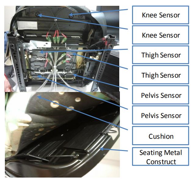
Erklärung zur Abschlussarbeit
gemäß §22 Abs. 7 und §23 Abs. 7 APB der TU Darmstadt

Hiermit versichere ich, Moritz Nottebaum, die vorliegende bachelor thesis ohne Hilfe
Dritter und nur mit den angegebenen Quellen und Hilfsmitteln angefertigt zu haben. Alle
Stellen, die Quellen entnommen wurden, sind als solche kenntlich gemacht worden. Diese
Arbeit hat in gleicher oder ähnlicher Form noch keiner Prüfungsbehörde vorgelegen.
Mir ist bekannt, dass im Fall eines Plagiats (§38 Abs. 2 APB) ein Täuschungsversuch
vorliegt, der dazu führt, dass die Arbeit mit 5,0 bewertet und damit ein Prüfungsversuch
verbraucht wird. Abschlussarbeiten dürfen nur einmal wiederholt werden.
Bei der abgegebenen Thesis stimmen die schriftliche und die zur Archivierung eingereichte
elektronische Fassung gemäß §23 Abs. 7 APB überein.
Bei einer Thesis des Fachbereichs Architektur entspricht die eingereichte elektronische
Fassung dem vorgestellten Modell und den vorgelegten Plänen.

Darmstadt, den February 25, 2020
                                                                     M. Nottebaum

                                                                                        1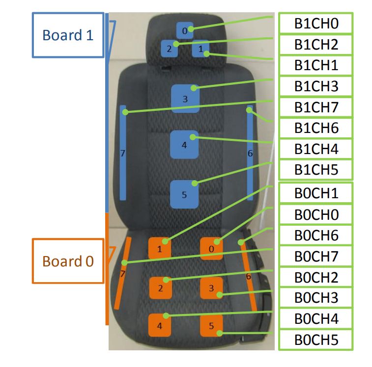
Abstract

In this thesis, I enhanced a car seat with 16 capacity sensors, which collect data from
the person sitting on it, which is then used to train a machine learning algorithm to
re-identify the person from a group of other already trained persons. In practice, the car
seat recognizes the person when he/she sits on the car seat and greets the person with
their own name, enabling various customisations in the car unique to the user, like seat
configurations, to be applied.
Many researchers have done similar things with car seats or seats in general, though
focusing on other topics like posture classification. Other interesting use cases of capacitive
sensor enhanced seats involved measuring the emotions or focusing on general activity
recognition.
One major challenge in capacitive sensor research is the inconstancy of the received data,
as they are not only affected by objects or persons near to it, but also by changing effects
like humidity and temperature. My goal was to make the re-identification robust and
use a learning algorithm which can quickly learn the patterns of new persons and is
able to achieve satisfiable results even after getting only few training instances to learn
from. Another important property was to have a learning algorithm which can operate
independent and fast to be even applicable in cars. Both points were achieved by using
a shallow convolutional neural network which learns an embedding and is trained with
triplet loss, resulting in a computationally cheap inference.
In Evaluation, results showed that neural networks are definitely not always the best
choice, even though the computation time difference is insignificant. Without enough
training data, they often lack in generalisation over the training data. Therefore an
ensemble-learning approach with majority voting proved to be the best choice for this
setup.
Keywords: Softbiometrics, Automatic identification system (AIS), Machine Learning,
Capacitive proximity sensing, Automotive

                                                                                             2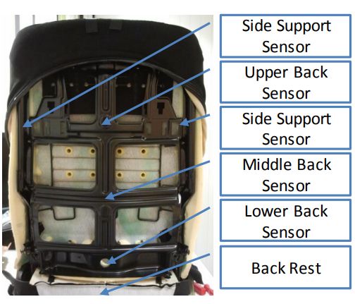
Contents

1   Introduction                                                                                                               5
    1.1 Goal . . . . . . . . . . . . . . . . . . . . . . . . . . . . . . . . . . . . . . .                                     5
    1.2 Overview . . . . . . . . . . . . . . . . . . . . . . . . . . . . . . . . . . . .                                       6

2 Related work                                                                                                                8
  2.1 Re-Identification . . . . . . . . . . . . . . . . . . . . . . . . . . . . . . . .                                       8
  2.2 Sensing Technologies . . . . . . . . . . . . . . . . . . . . . . . . . . . . . .                                        9

3 System Setup                                                                         12
  3.1 Hardware Setup . . . . . . . . . . . . . . . . . . . . . . . . . . . . . . . . 12
  3.2 Data Acquisition . . . . . . . . . . . . . . . . . . . . . . . . . . . . . . . . 15
  3.3 Seat Occupation Recognition . . . . . . . . . . . . . . . . . . . . . . . . . . 16

4 First Approach: Hand-crafted features                                                                                       17
  4.1 Feature Similarity Measure . . . . . . . . .        .   .   .   .   .   .   .   .   .   .   .   .   .   .   .   .   .   17
  4.2 Features selection . . . . . . . . . . . . . . .    .   .   .   .   .   .   .   .   .   .   .   .   .   .   .   .   .   18
        4.2.1 Mean . . . . . . . . . . . . . . . . .      .   .   .   .   .   .   .   .   .   .   .   .   .   .   .   .   .   19
        4.2.2 Fourier-Transformation . . . . . . . .      .   .   .   .   .   .   .   .   .   .   .   .   .   .   .   .   .   20
        4.2.3 Mean of the Fourier-Transformation .        .   .   .   .   .   .   .   .   .   .   .   .   .   .   .   .   .   21
        4.2.4 Extrema . . . . . . . . . . . . . . . .     .   .   .   .   .   .   .   .   .   .   .   .   .   .   .   .   .   22
        4.2.5 Ensemble-Learning . . . . . . . . . .       .   .   .   .   .   .   .   .   .   .   .   .   .   .   .   .   .   23

5 Second Approach: Triplet loss learning                                                                                      24
  5.1 Triplet-loss . . . . . . . . . . . . . . . . . . . .        .   .   .   .   .   .   .   .   .   .   .   .   .   .   .   24
  5.2 Classification . . . . . . . . . . . . . . . . . . .        .   .   .   .   .   .   .   .   .   .   .   .   .   .   .   26
  5.3 Training . . . . . . . . . . . . . . . . . . . . . .        .   .   .   .   .   .   .   .   .   .   .   .   .   .   .   27
      5.3.1 Neural Network loss . . . . . . . . . . .             .   .   .   .   .   .   .   .   .   .   .   .   .   .   .   27
      5.3.2 Selection of Data Points during Training              .   .   .   .   .   .   .   .   .   .   .   .   .   .   .   27
      5.3.3 Input Data processing . . . . . . . . . .             .   .   .   .   .   .   .   .   .   .   .   .   .   .   .   28
      5.3.4 Automatic Training . . . . . . . . . . . .            .   .   .   .   .   .   .   .   .   .   .   .   .   .   .   30

                                                                                                                               3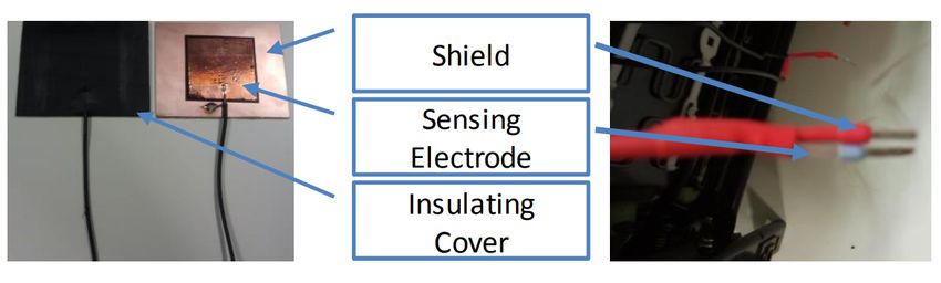
5.4 Neural Network Structure . . . . . . . . . . . . . . . . . . . . . . . . . . . 30
       5.4.1 Deep Neural Network . . . . . . . . . . . . . . . . . . . . . . . . . 31
       5.4.2 Shallow Neural network . . . . . . . . . . . . . . . . . . . . . . . . 32

6 Evaluation                                                                                 34
  6.1 Evaluation of Seat Occupation Recognition . . . . . . . . . . . . . . . . .        .   35
  6.2 Evaluation of Hand-crafted Features Approach . . . . . . . . . . . . . . .         .   35
       6.2.1 Total-Similarity Measure . . . . . . . . . . . . . . . . . . . . . . .      .   36
       6.2.2 Majority Voting . . . . . . . . . . . . . . . . . . . . . . . . . . . .     .   37
       6.2.3 Conclusion . . . . . . . . . . . . . . . . . . . . . . . . . . . . . .      .   37
  6.3 Evaluation of Triplet-loss Learning . . . . . . . . . . . . . . . . . . . . .      .   38
       6.3.1 Shallow Neural Network with normalized data . . . . . . . . . .             .   39
       6.3.2 Shallow Neural Network with feature input . . . . . . . . . . . .           .   39
       6.3.3 Deep Neural Network with standard input and normalized input                .   40
       6.3.4 Conclusion . . . . . . . . . . . . . . . . . . . . . . . . . . . . . .      .   40
  6.4 Result . . . . . . . . . . . . . . . . . . . . . . . . . . . . . . . . . . . . .   .   40

7 Conclusion and Future Work                                                                 42

                                                                                              4
1 Introduction
This research focuses on finding a suitable algorithm that is able to distinguish persons
by their sitting behaviour on a car seat. These characteristics are to be captured through
capacitive sensors. This topic is clearly useful in many scenarios. For example it could
automatically re-identify the driver and change the seat position. An infotainment system
could also automatically load a personalized account of the driver with all its configurations
of the car interiors. Identification in a car and in general is open to a lot usages in many
areas in times of IoT.
A notable advantage of capacitive sensors is not only their low price, but also their simple
and easy integration into various rigid objects like car seats [4] or non-rigid ones like blan-
kets [14]. Besides their cheapness and flexibility they can also operate on extremely low
amounts of current in contrast to cameras which could also be used for re-identification or
tracking in cars. Moreover the dimensionality of CPS (capacitive proximity sensing) data
is far easier to handle than camera picture data. Latter requires much more complicated
and computation intensive algorithms to extract the wanted information, especially in the
context of motion tracking, which of course relies on video data.
Interesting to know is that CPS technology is by far not new to the car industry [9]. There
are many applications of it in cars these days. One example is that some measure the
proximity of your hand to the door handle and initiate the unlocking process, when a
hand is near enough. Another example is the illumination of the infotainment screen,
when a hand advances to it.
1.1 Goal
Since researchers from the field of CPS technologies haven’t yet addressed the problem of
distinction of persons, it was difficult to define a concrete goal. Nevertheless the system
should fulfill some requirements that are needed to deploy it in a useful scenario. It should
be able to mitigate the inconstancy that is incorporated with capacitive sensing, such that
the precision of the identification does not depend on factors like weather and does not
5only work at specific temperatures and/or humidities. Especially when CPS is used in cars
the environment and with it the conditions can in short time vary dramatically.
In this thesis I predominantly focused on re-identification in a small group of people, but
trying to maximize accuracy in this constrained setting. self-speaking a car seat is primarily
occupied by a small number of people and recognizing a person simply by the data getting
from the second time they sat on the CPS enhanced car seat is not achievable by this setup
of sensors in my view. Thus focusing on re-identifying four to six people seems much more
reasonable. This constraint on the other hand leads to another desirable property namely
to have an uncertainty measure. The system should have some possibility to express if it
is not sure which class to pick in the classification process. As an ideal goal the algorithm
should classify a new person as unknown or should assess a known person which sits on
the car seat with a new unseen behaviour as also unknown instead of misclassifying him
or her.
Another major challenge of CPS for this task, is the circumstance that different clothing
can generate completely different sensor values, especially clothing like winter jackets
change the data notably due to their material and due to the different contact surface with
the seat, wherefore the system needs to be robust enough to handle such intra-personal
variance and maybe even learn these occasional inconsistencies in the data.
1.2 Overview
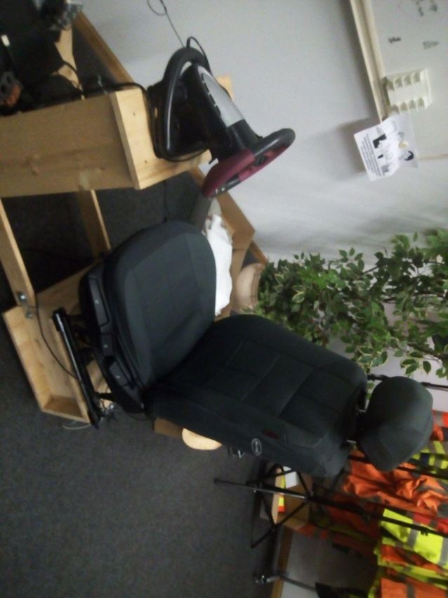
In Figure 1.1 one can see the whole setup. Only the seat contains sensors which send data.
The steering wheel is only used to let the testers have the feeling, that they are sitting on
a car seat. The testers always approach from the left side of the seat, as it would be in a
car. The seat is fixed to the wooden underground to prevent it from falling or shifting.
In the next chapter I will summarize the work, on which I build on. I differentiate my
related work into the topics of re-identification and sensing. In chapter 3 the system itself,
which is needed to properly get the data and be able to learn from it, is explained. In the
following two chapters I present the two approaches I tried. The first one was designed
without new machine learning techniques like neural networks, while the other used an
algorithm developed by Schroff, Kalenichenko, and Philbin. In chapter 6 I evaluate the
different approaches that were used and discuss the advantages and disadvantages of
each one.
Finally in the last chapter I conclude what was achieved in this thesis and try to predict,
what can be done in the future in this area to further improve the concept.
6Figure 1.1: System Setup of the Car Seat[5]
72 Related work
This thesis builds upon two research branches, namely re-identification and capacitive
sensing. At first sight these two areas do not seem to have much common ground, since
their application and purpose differs greatly. But it has often been shown, that some
algorithms and design choices that worked for specific tasks, could be applied to a vast
area of problems. The best examples are probably the widely used neural networks and
Principal Component Analysis (PCA), which both revolutionized many research fields.
On the other hand capacitive sensing predominantly changed how end consumers use
products such as mobile phones or even laptops. But this technology finds its way into
many applications and especially now, when machine learning algorithms constantly
improve and new are developed, CPS maybe can unfold its true potential.
2.1 Re-Identification
Re-identification is an important topic in the research communities. It is most commonly
known in the context of re-identification of persons on multiple cameras [18], or in the
context of IT-security with its various ways to give users,machines or objects an identity
by means of cryptographic algorithms [1].
The most promising beginning of re-identification in the context of classifying data was,
when Turk and Pentland used Principal Component Analysis (PCA) to extract the variations
of face pictures between different and same persons [17]. In order to identify and recognize
faces, they mapped them to a lower dimensional eigenvector representation and compared
different pictures in this low dimensional space by some arbitrarily distant metric.
This approach worked quite well and inference was comparatively cheap to compute, but
needed enough pictures of different faces to learn the possible variations beforehand. In
Figure 2.1 one can see the different eigenfaces (eigenvectors) to which a new face picture
is projected, resulting in a different representation of face images.
8Figure 2.1: The first picture on the left top is the mean face. The
other faces are the so called eigenfaces[8].
PCA is indeed mathematically very well-defined, as it actually captures the variation in
the data as much as needed and distinguishes data instances by their deviation from the
mean in the directions of the principal components.
But it lacks in identifying what variance in the data is really important for the distinction
of persons. For this reason Schroff, Kalenichenko, and Philbin achieved remarkable better
results with their embedding learning when applied to face clustering, recognition and
identification [15]. They wanted to learn this low dimensional feature representation
of data predominantly with the goal, that it specifically allows easy clustering between
different people.
2.2 Sensing Technologies
As already explained CPS has applications in many areas and especially research tries to
utilize them in manifold scenarios. One of the probably more unapplicable use cases was
explored by Laput et al., who achieved to recognize a firm amount of different objects by
touching them. The user would be required to wear a kind of glove, which was enhanced
with CPS, for this to be possible. The data from the capacitive sensors would be distin-
guishable, dependent on the material the object consists of and the mass of it [10].
9Most other applications of capacitive sensors are predominantly focusing on posture and
gesture recognition[4][3] on a car seat, except for example Grosse-Puppendahl et al., who
localized and identified people in a room through multiple long range capacitive sensors,
but lost accuracy, the more participants had to be distinguished [7].
On the other hand Sebastian Frank, who made the hardware setup I am using [5], suc-
cessfully utilized the car seat for posture recognition. . Since capacitive sensors, as later
described in section 3.1, can be used as a mixture of proximity and pressure sensing, the
field of Sebastian Frank seems very promising.
Figure 2.2: This is the 3D data from the Pressure Distribution Sensor
[16].
On the other hand Pickering et. al have a slightly different use case, which is simplified to
yield consistent results. They are demonstrating various use cases, where the car infers
through CPS, if the passenger or the driver are using certain controls in the car [13].
They do not try to identify the person itself, but rather can only distinguish between driver
and passenger.
Something very similar to what is an important part of my system, as later explained
in section 3.3, is already standard in many cars, namely an occupation recognition.
As described by Lucas et al., this recognition is used to enable or disable the airbag,
depending if a person sits on the car seat or not [12]. This safety-critical utilization of
CPS demonstrates, that even though the produced data is unstable and is influenced by
humidity and warmth, it is applicable to such problems, if it is done carefully and the task
is constrained.
Tan, Slivovsky, and Pentland tried to estimate the sitting posture through actual pressure
10sensors instead of CPS and classified data by using PCA, yielding pretty good results, but
lacking in generalization for unknown persons [16]. The data they received from the
pressure sensors can be seen in Figure 2.2. It is clear that pressure maps like this include
a lot of information, but their approach only incorporated a static analysis of the data and
didn’t consider the temporal changes, that are for example important for re-identification.
The reason for this, is that PCA can not simply be applied to high-dimensional data without
modification, because it works best with small data vectors and computation time explodes
otherwise.
There has indeed been much research in the direction of identification and in the direction
of capacitive sensors, but reliably identifying persons through these sensors and/or other
short range sensors with several possible users to re-identify, was still not tackled by
the research community, though there is a wide area of best practices and successful
algorithms in the context of capacitive sensing [6].
113 System Setup
In this chapter I outline what parts of the system needed to be implemented as the
framework for the re-identification to work. Independent of the algorithm used for
learning or inference, my System follows a certain sequence of steps. These steps are
repeated every second.
1. Data Acquisition (see section 3.2)
2. Seat Occupation Recognition (see section 3.3)
3. Inference or Data storing, depending on user Input(see chapter 4 or chapter 5)
Inference or data storing (learning) is only executed if the seat is occupied. To let the
system learn new identities or add data of already known identities, a learning command
and the name of the person need to be committed through a GUI. Then, if a person is
sitting on the seat, the third point from the cycle above is executed and thus the data of
the sitting person is stored under the name, which was committed (for more details see
section 3.3). In practice, when this system would be applied to a car, the learning is done
through a identification of the user through voice recognition for example. When a user
sits the first time on the seat, the name needs to be typed in somewhere.
3.1 Hardware Setup
Capacitive sensors can colloquially be abstracted in this setup (Figure 3.1) as a mixture of
proximity sensing and pressure sensing. The closer an object gets to it, the higher is the
sensor value. The same holds for pressure, resulting in a even higher value.
Hence algorithms are able to interpret the data and measure how far a person is away
as well as how much pressure it creates on the chair (for more details in this special
domain please read Sebastian Franks work, as he also focused on measuring distances
with capacitive sensors [5]).
12In contrary to him, my goal was not to translate the measurements into actual distances,
but rather let the algorithm itself interpret the data with its own measures.
In the setup described in the next paragraph the value range of CPS differs greatly, de-
pendent on how they were integrated into the car seat, as well as their general sensitivity
for proximity and pressure. Handling those non-linear differences between the sensors
requires enough data to learn the individual properties, such that the algorithm can inter-
pret it correctly.
Figure 3.1: Sensor Setup of the car seat[5]
Since Sebastian Frank already evaluated what sensor setup is suitable to capture different
human motions on a car seat, I could use his work as the baseline of my thesis[5]. As can
be seen in Figure 3.1 the sensors are split into two sensor groups, the backrest and the
seating surface, each one equipped with eight sensors.
Sensor six and seven in both groups of the car seat are especially important, since they
capture the approach of the person, when they start to sit on the seat, as well as the
13width of the sitter. Sensors zero to five in the seating surface are predominantly meant to
recognize the contact points of the sitting person, as well as the pressure created by the
person through their individual weight.
On the other hand the zero to two in the headrest are designed to capture how often and
intensive the head is leaned in the direction of that part of the chair. Sensors three to five
in the backrest follow the same idea, but measure the intensity of the pressure from the
back to the backrest.
Figure 3.2: Sensor positions in the backrest of the car seat [5]
In Figure 3.2 one can see the backrest of the seat from behind. The five sensors, that are
incorporated into the backrest, are put between the metal frame and the cushion. With
this design, they are exposed to possible pressure effects from the front of the seat.
In Figure 3.3 it is portrayed how the sensor is shielded from one side. This is needed,
because otherwise the metal frame would influence the sensor and make its values very
unstable and thus useless for any recognition algorithm. For a more detailed description of
the hardware setup and shielding please look at Sebastian Franks work [5], as he designed
all of it.
14Figure 3.3: Sensor shielding from unwanted disturbances [5]
As can be seen in Figure 3.4 the seating surface is equipped with sensors similar to the
backrest, as they are again placed between the metal and the seat cushion, offering the
same advantages as said before.
Figure 3.4: Sensor incorporation in the seating surface [5]
3.2 Data Acquisition
As already mentioned Sebastian Frank [5] constructed the sensor setup that I utilize for
this thesis, but I did not use his Data Acquisition framework. The communication with the
sensor boards was programmed in Java, where I included code parts from the plotter of
capacitive sensors from the Fraunhofer IGD. This part of my software works as a client
15which connects to a server written in python. It sends the data received from the sensors
in a one second interval to the python server.
The data of one second is approximately an array of size [25 × 16]. 16 corresponds to the
number of sensors and 25 is the number of data points each sensor sends in this interval
(the value 25 can vary). The data acquisition can be described as follows:
1. Subtract the bottom-value of each sensor from the new data points (the bottom value
is calculated from the first data received)
2. Store it in a data array, that saves at least the last five seconds of data
One data point which is used as learning data consists of three seconds which is an array
of size [75 × 16].
3.3 Seat Occupation Recognition
The first logic part of my code was self-speaking the occupation recognition, as it was
mandatory to even gather data to learn from. Without the system knowing, when the
person starts to sit on the seat, the data would not be collected from exactly the same
point of time in each learning phase. For recognition to work, the system must know which
part of the received data is important, namely knowing the interval of the data, starting
right before the person starts to sit and ending after the next three seconds from there.
The seat occupation recognition simply checks, if four sensors at the same time exceed
a certain threshold value. As can be seen in section 6.1 this is enough to have a very
robust seat recognition. It is also aware of the difference between the sensors sensitivities,
because as described in section 3.2 the bottom of the possible sensor values (when no
person is sitting) is sensor-specifically subtracted in the data Acquisition part before further
processing. The above-named threshold on the other hand is the same for all sensors,
which is not a perfect solution, but more than sufficient for this task.
164 First Approach: Hand-crafted features
Since the concept of this thesis was to create a system, that can identify persons with
very few data available, neural networks and deep learning wasn’t an option at first, as
this usually requires a lot more data. Independent from the fact, that getting the data in
this scale would disrupt the time frame of this thesis, it would not have been practical
in real life scenarios. That’s because retraining it for each user would be inevitable if
we use a standard classification network and thus making it impossible to apply in real
cars, especially because the person which should be re-identified would have had to sit
thousands of times on the seat, before the neural network could recognize him or her with
sufficient precision. In addition the training needed to be done automatically.
All of these factors make it implausible, wherefore I didn’t deepened work in this direc-
tion at the beginning. In chapter 5 I used a different learning technique from Schroff,
Kalenichenko, and Philbin [15] to work around the problems just described. But even
when using new techniques, learning can be difficult, not robust enough and/or be exposed
to overfitting.
With all this in mind I therefore tried to accomplish the re-identification by using hand-
crafted features and distinguish persons by comparing those.
4.1 Feature Similarity Measure
In order to compare feature vectors of different persons with the received data from the
person sitting in the seat, I needed a similarity measure to compare features efficiently
and robustly. Since the numerical magnitudes of the different possible feature categories
shouldn’t influence their importance, when using more than one feature for comparison,
I had to use a mathematical solution that can compare two feature vectors of the same
category and describe their similarity as a value between zero and one. As cosine similarity
17fulfilled these requirements completely it was the perfect choice for this part of my system.
Let A and B be two feature vectors, then cosine similarity is defined as follows:
A·B
simcos (A, B ) = (4.1)
∥A∥2 ∥B∥2
The feature vectors are stored in the three dimensional matrix F which can be formally
defined as follows where M is the maximal feature size, N the number of features and D
the number of data points:
F ∈M ×N ×D (4.2)
F can be indexed as Fij where i defines the feature category and j the data point. F is
three dimensional because one dimension belongs to the feature vector itself. As explained
in section 3.2 each data point consists of the sensor data collected in three seconds. When
evaluating the similarity or distance of two data points, each feature of both data points is
compared with cosine similarity, resulting in the following total similarity measure, where
j and k are the indices of the data points that get compared.
N
1 ∑︂
totalsim(j, k ) = simcos (Fij , Fik ) (4.3)
N i=1
The re-identification result is then the person to whom the stored data point with the
highest total similarity belongs.
This classification procedure could be enhanced with a k-nearest neighbor approach, that
classifies with respect to the k highest similarity scores. The already learned person with
the most data points that belong to the k biggest similarity scores is then the classification
result. This enhancement is tried with the automatic feature generation from the neural
network as later explained in chapter 5. In chapter 6 k-nearest neighbor is evaluated as a
possible part of an hand-crafted feature classification.
4.2 Features selection
Now that we talked about the framework in which we use different features for classifica-
tion, the actual selection of those is much more intricate.
Since we have 16 sensors implemented in the seat, the features are at least vectors of this
size. As pointed out in section 3.2 every sensor is given its own time series, consisting of
1875 values, which we want to convert to a lower dimensional representation (feature) that
is invariant to small changes in the data, but stays discriminative enough to be useful.
It’s important to note that having too many features is not expedient. One reason for
this is, that if two lower dimensional representation of data overlap in what they extract,
this overlapped part gets a higher significance in the classification decision because it is
weighted higher as it occurs in two comparisons of two data points. Too many features
contradict the idea of a low dimensional representation of data whose sense is to reduce
overfitting. Overfitting can occur if all the details are caught in the data, preventing the
features to generalize over the data. Our approach doesn’t want to learn the data, but
rather the generalization of it, such that it can categorize new data.
4.2.1 Mean
The time series can be seen as a function. One important property of a function can be its
distance to the x-axis, also known as y-shift. In our case the mean distance to the x-axis is
more interesting, as the y-shift at the beginning of our function/data doesn’t carry that
much valuable information. Since the data is non-negative this simply translates to the
mean value of the data.
In other words the mean captures the magnitude of the time series. So in practice we turn
an array of size [75 × 16] into a feature vector of size [16], where each number corresponds
to the mean value of the time series of one sensor.
To show that the mean is a sensible feature I plotted the mean of the mean of each person
for each sensor in Figure 4.1. To explain it in more detail, as described above each data
point, when extracting the mean, results in a feature vector of size [16]. I then averaged
over all this vectors for each person separately, resulting in nine feature vectors of size
[16], because I have nine classes/persons as data. For visualization I cut off just a few
mean values of the data as they had a too high value to show them all in one plot. For
each person there are at least twelve data points, from which the mean of the mean was
computed, making this figure indeed meaningful.
As can be seen some sensors do not offer that much differentiation through mean as a
feature, but others do quite well, like sensors one, two, seven, eight and fifteen. And some
can distinguish between a few classes. It can of course also be seen that the mean alone
is by far not distinctive enough for most classes/persons, leading to our next feature. Of
course this plot does not really proof anything, but it gives the intuition, that mean indeed
can be a good feature. Practical evaluation in the end, is the tool to choose to actually
proof its reliability (see section 6.2).
19Figure 4.1: Each point represents the mean of the mean of all data points of each person
for each sensor, where the color denotes the person and the x-axis the sensor.
4.2.2 Fourier-Transformation
Another possible property of a function is how it’s shaped. In other words, what it looks
like and how it goes up and down. This part can for example be captured by a Fourier-
Transformation of the data. Since the data is discrete, the Discrete Fourier Transformation
must be used. Hence for each sensor curve we get some firm amount of Fourier parameters
that can be compared through the cosine similarity measure. The number of parameters
the transform outputs can be specified.
In my system I only used ten Fourier parameters for each sensor and data point, but as
can be seen in Figure 4.2 this is sufficient to pretty accurately define the curve of the
function/data. To create the left functions you first need to make a Fourier-Transformation
of the data on the right and then only take ten Fourier parameters from that and make an
inverse Fourier transformation, resulting in the left curve in Figure 4.2.
In the end we get a matrix of size [20 × 16] for each data point as a feature, because
each Fourier parameter is made of a real and imaginary part. Since the cosine similarity
is not properly defined for complex numbers, I simplified this problem by making the
imaginary part of each of the ten parameters an own number, thus doubling the number of
parameters. In practice the matrix of size [20 × 16] is self-speaking converted into a vector,
as cosine similarity can not work with matrices.
20It seems clear that this approach has weaknesses, as this feature is not properly mathe-
matically defined, is ambiguous, not distinctive enough and prone to overfitting because
of its size. In section 6.2 I will evaluate, if it nonetheless is a practical and useful feature.
The problem is that cosine similarity is linear, while the Fourier-Transformation is highly
non-linear. The Fourier parameters do not change linearly to the curve they describe.
More specifically, if the curve changes a bit, the Fourier parameters may differ greatly, as
they each describe a sinus or cosine part and it is not predictable, which wave is used for
which part of the curve.
Figure 4.2: On the right is the original data of one sensor (75 sensor values) of two different
data points. The data bottom is already subtracted (see section 3.2). On the
left is the inverse transformation of the Fourier-Transformation of the original
data from the right using only 10 of the 75 Fourier parameters.
4.2.3 Mean of the Fourier-Transformation
As explained before in subsection 4.2.2, features consisting of too many numbers can
lead to overfitting. Thus using the mean of the Fourier-Transformation combines the
distinctiveness of the Fourier-Transformation and the robustness of the mean operator.
21So instead of having [20 × 16] numbers as the feature of a data point, its size is reduced
to [16]. Averaging over the Fourier-parameters should also mitigate the problem of their
non-linearity. This is the case, since the non-linear change of a Fourier-parameter does
only little change the mean of all parameters.
In subsection 4.2.1 we used the plot in Figure 4.1 to show the potential of distinctiveness,
encapsulated in the mean as a feature. I did the same in Figure 4.3 for the mean of the
Fourier-Transformation, yielding comparable results. Again keep in mind that, I had to cut
off some parts of the plot, since otherwise the differences between the classes would be
more difficult to see. Some sensors lead on to very high mean values.
Figure 4.3: Similar to Figure 4.1, each point represents the mean of the mean of the
Fourier parameters of all data points of each person for each sensor, where
the color denotes the person and the x-axis the sensor.
4.2.4 Extrema
In subsection 4.2.2 I enlarged upon the intuition, that the Fourier-Transformation already
captures the form of the curve as a feature. But since the curve of the data is the most
important part to reliably distinguish between different persons, several strategies need to
be tested and evaluated.
Extremas as a feature seems promising, since they are extremely significant properties of a
function. As can be seen in Figure 4.2, the curves consist of several extrema and they are
22at different positions and have different heights. The training data periodically goes up
and down (as the sitting behaviour of humans is generally periodic in the normal direction
of the seat surface) , thus when describing it through the maxima, a decent proportion of
information of the data can be captured.
Important properties of it are position and height. The resulting feature of one data point
has the size of [16 × 2]. The first part of it is the number of peaks of each sensor curve, the
second is the mean height of the peaks of each curve.
4.2.5 Ensemble-Learning
In section 4.1 the framework is described, in which several features can be combined
to measure a similarity between two data points. The problem of this kind of similarity
measure, when comparing more than one feature, is that the similarity of one feature
influences the similarity of another one, because all similarities get summed up and divided
through the number of used features (seeEquation 4.3 ).
In many fields of Machine Learning, some kind of discrete handling of a higher dimensional
problem can be helpful (graph cut is a good example for this [2]). In respect thereof I try
majority voting of the different features to determine the resulting class.
For this to work, every feature votes for a class alone, resulting in an array of size N , where
N is the number of classes.
votes := [v1 , ..., vN ]
where vi is the number of votes for class i
class = argmax(votes[i])
i∈[1,...,N ]
Self-speaking most entries in the array will be zero except of the votes. The vote result
comes from the cosine similarity measure from Equation 4.1. The class of the data point
with the highest similarity from all data points, is the class for which each feature votes.
When two classes have the same number of votes, the classification predicts it as unknown
and thus it counts to the wrongly classified examples. In section 6.2 I will evaluate
if Ensemble-learning with discrete majority voting yields better results than the total
similarity from Equation 4.3. In this classification framework k-nearest neighbor is not
used, in this setting only the nearest neighbor decides for which class the feature votes.
235 Second Approach: Triplet loss learning
As pointed out at the beginning of chapter 4, simply using a neural network won’t work,
as it is required for this system to be meaningful, that it is able to learn a person after a
few times he or she sat on the seat. This is impossible for a usual neural network, even if it
is fairly shallow. Classification tasks of this kind need much more training data to properly
learn something. If we assume a simple convolutional network with for example seven
layers and a softmax output function where the ground truth is a one-hot coded vector
representing the class/person, another problem arises namely that the whole network
had to be retrained, if a new person has to be recognized. This makes a standard neural
network of this kind unsuitable for my application.
In chapter 4 I selected features that seemed distinctive and robust to me, but learning
features almost always yields to better results than hand-crafting them, if enough data is
available. Triplet-loss does exactly that, it learns a lower dimensional representation of
the data instead of simply classifying it [15].
This solves the retraining-problem, when new persons are to be learned by the system,
as the neural network should ideally generalize well in how to convert similar data into
sensable feature vectors, even if the data comes from a completely new person. And
when new persons should actually be learned, the network structure doesn’t need to
be changed and thus it doesn’t have to be completely retrained, though in part further
training probably needs to be done.
These low dimensional representations can then be compared with other low dimensional
representations from anyone who sat on the seat, although the neural network never
learned the data from that person (see section 5.2).
In section 5.1 we will see why the few data points per class pose a smaller problem, when
using Triplet-loss training.
5.1 Triplet-loss
The idea of triplet-loss training is to learn a low dimensional representation of the data,
also called embedding [15]. It tries to maximize the euclidean distance of the embedding
24from data points of different classes and minimize the distance of data points belonging
to the same class. It tries to create this euclidean space that allows easy clustering of data,
according to how the classes are assigned to the data. This in theory converges to a space
where the distance between two data points (after forwarding them through the neural
network) is determined by the belonging to a class and not simply by the difference of the
sensor values. If both spaces, the initial and the desired (the one to learn), would be the
same, classification could be done by using the euclidean distance. But in general this is
not the case.
This is achieved through the loss function in Equation 5.1, that replaces the usual cross-
entropy as loss. In Equation 5.1 xai is the anchor, which is the embedding of the current
data point that was forwarded in the neural network, xpi is the embedding of the data
point of the same class, that is farthest away from the anchor, and xni is the embedding of
the data point from a different class, that is the closest to the anchor embedding and N is
the number of data points.
N [︃
∑︂ ]︃
a p 2 a n 2
L= ∥f (xi ) − f (xi )∥2 − ∥f (xi ) − f (xi )∥2 + α (5.1)
i +
Through this loss the neural network learns the embeddings. These low dimensional
representations of the discrete input data allow classification simply through any distance
metrics in the euclidean space. For this thesis I simply used the euclidean distance to
classify the data points. Since the loss is not determined through one data point, but rather
three, the training data is more utilized than with usual training procedures, as the loss
and the back-propagation has more variety, because there are principally N 3 ( the anchor,
the positive example and the negative one) possible input constellations for triplet-loss.
Choosing the hard negatives and positives
Schroff, Kalenichenko, and Philbin did emphasize that the right choosing of xni and xpi
is important. When only taking the negative example xni with the greatest distance to
the anchor xai , that could make the model collapse and end in bad local minima during
training [15]. Thus it is recommended to choose a negative example, that fulfills the
following equation:
∥f (xai ) − f (xpi )∥22 < ∥f (xai ) − f (xni )∥22 (5.2)
This constraint ensures that not always the worst outlier (the negative example closest to
the anchor) is chosen as xni . Accordingly single training data points, that often appear as
such, do not influence the learning disproportionate. Otherwise it would very probably
ensue, that the model overfits to certain data points.
25From all negative examples xni , that fulfill the Equation 5.2, a random one is then used for
the loss from Equation 5.1.
5.2 Classification
As mentioned in section 4.1 using k-nearest neighbor seemed promising for classification,
as data from the same person still can differ very much depending on how the person sits
on the chair and some seating behaviours of different persons may be similar. This is why
not only the nearest data point can be interesting, but rather the eight or ten nearest, in
order to capture different seating behaviours of the same person, as the neural network is
by far not perfect in this.
Classification can then be outlined as follows in algorithm 1, where net represents the
neural network, to which data can be passed and the output of the network is returned.
The data, that shall be classified, is the array newdata, while alldata is a list of all data
points of each person, that were stored and already used for training.
Algorithm 1 Classification
1: procedure classify(newdata, net, alldata,k)
2: new_embedding ← net(newdata)
3: known_embeddings ← empty_list
4: for each datapoint from alldata do
5: known_embeddings.add(net(datapoint))
6: end for
7: k_closest ← get_k_closest(k, known_embeddings, new_embedding)
8: result ← most_frequent_class(k_closest)
9: return result
10: end procedure
The method get_k_closest in algorithm 1 uses the euclidean distance to get the k clos-
est embeddings needed for k-nearest neighbor classification. Important to note here is
that the system, as long as it hasn’t been learning only once needs to compute the list
known_embeddings.
The method most_frequent_class simply returns the class that appears the most fre-
quently in the list k_closest. If two or more classes occur equally often then the resulting
category is "Unknown". K-nearest neighbor classification thus allows to measure some
kind of uncertainty of the algorithm.
265.3 Training
For training there are several hyperparameters to choose, like batch size and learning rate.
During training the latter constantly has to change, to find a good local optimum. For this
system to be applicable, for every new car, it has to be retrained with the new persons
sitting on it (the car owners). To make this possible some kind of automatic training needs
to be done, that can reliably achieve sufficient precisions (see subsection 5.3.4).
In the following subsections I will also describe different possible ways to influence the
outcome of the training. In section 6.3 I will evaluate the combination of various ways to
learn the training data and elaborate which one to use. The batch size is also constant for
all versions of the training, in order to allow comparison. It is fixed to 15.
5.3.1 Neural Network loss
Besides the loss described in section 5.1, other information has to be added to the total
loss, in order to ensure specific constraints and/or prevent overfitting. In the triplet-loss
paper[15] they recommend to constraint the output of the network with the euclidean
magnitude of ∥f (x)∥2 = 1, where f stands for the neural network and x is the input data.
Another important addition to the loss is a L2-regularization term, which ensures that the
summed magnitude of the parameters of the network stays constant. I constraint it to a
value of one. L2-regularization is a common way to prevent overfitting and is widely used.
Both enhancements of the loss are utilized for every of version of my network.
5.3.2 Selection of Data Points during Training
A very important part of training is, deciding in what order the data is chosen for forwarding
through the neural net. I thought of two possibilities, which both have advantages and
disadvantages, but are both applicable and achieve good results.
Random ordering
Instead of just doing training with the same ordering of the input data every time, I
randomly shuffle the array, which defines in which sequence the data points get forwarded
through the network, every epoch. The problem of this is, that not every class has the
same number of data points, and in this way some classes get preferred in the training.
27On the other hand the difference is not significant and is maximally in the range of 10
percent of the number of training data points of a class.
Uniformly distributed between classes
To work around the problem of random ordering of section 5.3.2, I instead could for every
training iteration randomly sample a number from a uniform distribution with the domain
[1, ..., N ] where N is the number of classes. This number would define the class of the data
point. To then determine which data point to choose from the class, a number is sampled
from another uniform distribution with the domain [1, ..., Ci ], where Ci is the number of
data points of class i.
Conclusion
The problem with the uniformly distributed between classes approach is, that the ran-
domness can lead to the problem, that some data points are forwarded less frequent than
others. Furthermore the training is not reproducable and unstable. The random ordering
is the perfect balancing between bringing some randomness into the model, while also
ensuring quite stable training in each epoch.
5.3.3 Input Data processing
When using neural networks, some kind of normalization of the data can be useful, or is
even a prerequisite for it to work. In section 3.2 I explain how the raw data of the sensors
is processed, but above that there are several additional ways to improve the fit of the data
for the neural network. In the following I will describe two different ways to process the
input data.
Normalization
Even after subtracting the minimum value of each sensor from the data, their maximum
value can still be a five-digit number. Since all versions of my neural network use the
tangens hyperbolicus as an activation function, the input, no matter how high, will be
reduced to maximal one after the first layer.
282
Figure 5.1: The Tanh-function is defined as tanh(x) = 1 − e2x +1 .
In Figure 5.1 the tanh function is displayed and as can be seen all inputs above x = 3 have
approximately the same value (input consists only of positive inputs). Thus some kind
of normalization can be useful to ease the handling of the data for the neural network.
There are of course several other reasons which are described in detail in the paper from
LeCun et al. [11]. He recommends the following normalization described by the informal
math, where x stands for the whole input data:
m = mean(x)
σ = stddeviation(x)
x = (x − m)/σ
Through this the training data gets a mean of zero and a standard deviation of one, making
it more suitable to a neural network.
Feature Extraction
Aside from techniques aimed to make the data fit the neural network, another approach is
to first extract some features such as mean and standard deviation and feed them to the
neural network instead of the input data. For this thesis I used the features mean, mean
of the Fourier-Transformation and extrema. I extract them just as described in section 4.2.
295.3.4 Automatic Training
As elaborated before, automatic training is crucial for this system to be practically usable.
All versions of my neural network use the same automatic learning strategy. After every
epoch the current parameters of the network are stored in a folder. Thus this generates a
big pool of training saves with which further training can be done. The following steps
are done to get to the final result.
1. Neural network randomly initializes its parameters.
2. The neural network trains until it reaches epoch 100.
3. It randomly selects any training save from the corresponding training, that fulfills
the following requirements:
a) Its precision on the validation set must not differ more than 2.5% from the
maximum of all training saves.
b) Its precision on the training set, must not differ more than 8% from its precision
on the validation set.
4. The learning rate is multiplied with 0.8 and thus decreased.
5. Goes to the second point and initialize the parameters of the neural network with
the chosen training save.
The first Requirement from point 3 is obviously needed to push precision, while the second
is crucial to prevent overfitting. Of course both numbers mentioned above, are variable
and were specially chosen from me for my models.
5.4 Neural Network Structure
In the following I will show and explain the two main versions of my neural network.
Both architectures were refined by me, based on their results. Both neural networks use
the Tanh-function as activation function as mentioned in section 5.3.3. During testing it
achieved better results than the usual sigmoid.
The first approach was to try a deeper convolutional neural network with six layers. The
structure of it can be seen in Table 5.1. The second Approach is a more shallow neural
net with just four layers. The idea for this one came from Philipp Terhörst a scientific
collaborator at the Fraunhofer IGD. The data acquired from the sensors is, even though it
is quite high dimensional, not as complex as that of a picture for example. This can be
30easily confirmed when looking at Figure 4.2. The actual information from one curve is not
high dimensional, thus using a shallow neural network without convolutional layers is
indeed also a very promising attempt.
5.4.1 Deep Neural Network
In this deeper neural network the first fully connected layer fc1 receives not only the
output from the pooling-layer pool3, but also the activations of pooling-layer pool1. The
size-in number from layer fc1 emerges from the addition of both layer outputs resulting
in 15 × 149 + 30 × 17 = 2745 neurons. This architectural decision is called Skip-connection
and is used in many state-of-the-art neural networks, proofing to be very beneficial.
The problem is, that this increases the amount of parameters in layer fc1 quadratic and
thus gives rise to overfitting. To counteract this, I used three dropout-layers (not shown in
Table 5.1) with p = 0.5. They are placed after every fully-connected layer.
The idea of the convolutional layer here, is that they extract important features out of the
data and forward them to the fully-connected layers, that then transform them into the
desired euclidean space described in section 5.1. The desired space is 10-dimensional in
all networks. This is given by the fact, that the last layer has ten neurons.
layer size-in size-out kernel param
conv1 1200 15 × 589 5, 2 90
pool1 15 × 589 15 × 149 4, 4 0
conv2 15 × 149 30 × 147 3, 1 1380
pool2 30 × 47 30 × 36 4, 4 0
conv3 30 × 36 30 × 34 3, 1 2730
pool3 30 × 34 30 × 17 2, 2 0
fc1 2745 1372 3.7M
fc2 1372 343 470K
fc3 343 10 3.4K
total 4.177M
Table 5.1: This table shows the structure of the neural network, where size-in and size-out
is described by channels × length. The Kernel on the other hand is described
by size, stride .
315.4.2 Shallow Neural network
There are two versions of the shallow neural network, one that accepts the usual data as
input and one that accepts extracted features of the data as input (see subsection 5.3.3).
In Table 5.2 the neural network with the feature input is depicted. As said before I use the
features mean, mean of the Fourier-Transformation (FT-mean) and extrema as input. As
shown in section 4.2 the extracted properties mean and FT-mean are each of size 16 and
extrema of size 32, resulting in the total input size of 64.
The advantage of this attempt is clearly that by far fewer parameters are needed. The
theoretical disadvantage is, that the extracted features reduce the amount of information
the neural network gets. This includes a bias into the training, which can be beneficial,
when not having enough data. Though a bias can also cap the potential of it.
layer size-in size-out param
fc1 64 64 4K
fc2 64 32 2K
fc3 32 16 528
fc4 16 10 170
total 7K
Table 5.2: This table shows the structure of the smaller neural network with features as
input.
On the other Hand in Table 5.3 is the structure of the same neural network, just with a
higher amount of input numbers. This means more input neurons are needed and thus
the following layers also needs more of them to have a plausible architecture. Compared
to Table 5.1 it has a forth of the parameters.
Nevertheless it has to train a lot more parameters than the other shallow one, thus is
much more prone to overfitting. Just as in the deep network I use dropout in both smaller
networks with p = 0.4. All architectures have their pros and cons, thus they need to be
evaluated in practice to find the best-fitting model for the problem (see section 6.3).
32layer size-in size-out param
fc1 1200 600 720K
fc2 600 300 180K
fc3 300 150 45K
fc4 150 10 1.6K
total 947K
Table 5.3: This table shows the structure of the smaller neural network with the unpro-
cessed data as input.
336 Evaluation
My dataset consists of nine different classes/persons. The data points per class can be seen
in Table 6.1. During my evaluation I always use half of my data of each class as training
set and half as validation set, such that each class has a validation and training part of the
data. This is independent of whether the neural network or the hand-crafted features are
evaluated. Even though more training data would definitely improve the learning result
of the neural net, they have to have the same starting ground, because in practice training
data is not abounding. Also the validation set needs to be big enough to have a sensable
validation precision. Another important property of my evaluation is, that the belonging
of data points to validation or training set is constant throughout all evaluated approaches
to ensure consistency.
Moritz Niklas Tina Thomas Timm Nils Antonia Bennet Timo Total
47 45 39 30 45 43 50 50 42 392
Table 6.1: This table shows the data points per class.
Since the data points per class differ, all overall precision values are normalized precisions
in this evaluation. The definition of it is the following. Here x is an array defined as
[x1 , ...xN ], where xi is the precision of class i and N is the total number of classes:
N
1 ∑︂
norm_prec(x) = xi
N i=1
The difference of the usual overall precision, to the above defined is, that in the usual one
simply the number of right classifications is divided through the total number of classified
data points, leading to a precision, that is dependent on the number of data points per
class. Thus if a class, that in general has a higher precision, holds more data than other
classes with worse precisions, than the overall precision would be pushed higher due to
the better class, even though the algorithm fails at classifying the other classes. Since the
34objective is to achieve good precisions on all classes, normalized precision is the evaluation
measure to use.
6.1 Evaluation of Seat Occupation Recognition
From the rough 392 times people sat on the chair during data collection, the seat occupation
never failed in recognizing that a person is sitting. Only with extreme effort and pressure
on the seat, it is possible to trick the system. Thus it results a precision of 100%.
6.2 Evaluation of Hand-crafted Features Approach
In the hand-crafted Features approach we distinguished between Majority voting (see
subsection 4.2.5) and total-similarity measure (see section 4.1). We will evaluate both
based on the presumption, that mean, FT-mean and extrema are the best features for both
approaches. I presume that they are, independent of the training and validation mixture
of the data. I validated any combination of three features for the total-similarity measure
and the majority voting. The results can be seen in Table 6.2. The five best combinations
are depicted there.
total-similarity m,e,ft m,mm,e m,ft,mm m,std,ft m,mm,std
overall precision 0.78 0.76 0.75 0.74 0.73
majority voting m,e,ft ft,mm,e e,mm,m mm,ft,m adm,e,m
overall precision 0.74 0.74 0.72 0.71 0.71
Table 6.2: All values are rounded to the second figure after the
decimal. In the table (m) stands for mean, (e) for extrema,
(ft) for mean of the Fourier-Transformation, (mm) for
min-max, (std) for standard deviation and (adm) for
median absolute deviation.
From Table 6.2 it cannot be deducted that mean, FT-mean and extrema are in general the
best features for every possible training and validation data constellation, but they still
seem the most promising. It can also be assumed at first, that total-similarity is superior to
majority voting , at least for this constellation. It makes sense that these three properties
of the data work best. Mean catches the amount(intensity) the sensors get, FT-mean the
average curve and extrema the upper bound of it. The lower bound is not distinctive as
35You can also read