Robust dynamic community detection with applications to human brain functional networks - Nature
←
→
Page content transcription
If your browser does not render page correctly, please read the page content below
ARTICLE
                  https://doi.org/10.1038/s41467-020-16285-7                 OPEN

                  Robust dynamic community detection with
                  applications to human brain functional networks
                  L.-E. Martinet1,5, M. A. Kramer                2,3,5,   W. Viles2, L. N. Perkins            4,   E. Spencer       4,   C. J. Chu1, S. S. Cash1 &
                  E. D. Kolaczyk 2 ✉
1234567890():,;

                  While current technology permits inference of dynamic brain networks over long time per-
                  iods at high temporal resolution, the detailed structure of dynamic network communities
                  during human seizures remains poorly understood. We introduce a new methodology that
                  addresses critical aspects unique to the analysis of dynamic functional networks inferred from
                  noisy data. We propose a dynamic plex percolation method (DPPM) that is robust to edge
                  noise, and yields well-defined spatiotemporal communities that span forward and backwards
                  in time. We show in simulation that DPPM outperforms existing methods in accurately
                  capturing certain stereotypical dynamic community behaviors in noisy situations. We then
                  illustrate the ability of this method to track dynamic community organization during human
                  seizures, using invasive brain voltage recordings at seizure onset. We conjecture that
                  application of this method will yield new targets for surgical treatment of epilepsy, and more
                  generally could provide new insights in other network neuroscience applications.

                  1 Department of Neurology, Massachusetts General Hospital, Boston, MA 02114, USA. 2 Department of Mathematics and Statistics, Boston University,

                  Boston, MA 02215, USA. 3 Center for Systems Neuroscience, Boston University, Boston, MA 02215, USA. 4 Graduate Program in Neuroscience, Boston
                  University, Boston, MA 02215, USA. 5These authors contributed equally: L.-E. Martinet, M. A. Kramer. ✉email: kolaczyk@bu.edu

                  NATURE COMMUNICATIONS | (2020)11:2785 | https://doi.org/10.1038/s41467-020-16285-7 | www.nature.com/naturecommunications                           1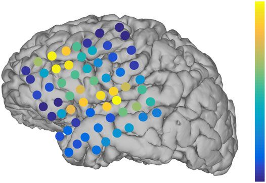
ARTICLE                                                                 NATURE COMMUNICATIONS | https://doi.org/10.1038/s41467-020-16285-7

T
        he brain functions (and dysfunctions) through interactions           seizure onset, suggesting the potential for targeted therapeutic
        spanning spatial scales, from the single neuron to the entire        intervention.
        nervous system, and temporal scales, from millisecond
action potentials to decades of development1. Modern neuroi-
maging, combined with sophisticated data analysis tools, has                 Results
expanded analysis of brain activity from individual brain com-               The DPPM. The DPPM operates on dynamic networks, which
ponents to networks of interacting brain regions. Understanding              may be inferred from noisy time series data. Before illustrating
these brain networks (e.g., the connectome2, dynome3, and                    the utility of this method in simulation and examples of obser-
chronnectome1), and the big data they entail, remains a funda-               vational data, we first briefly describe and motivate the proposed
mental challenge of modern neuroscience4, with the potential for             dynamic community detection procedure.
significant impacts to human health and disease5,6.                              Let G = (V,E) be a graph with vertex set V and edge set E, and
   Initial research efforts have focused on characterizing properties        let fGt gNt¼1 denote a sequence of N graphs indexed by time t,
of isolated brain networks using static graph metrics, resulting in          which we assume to share a common vertex set V. Our goal is to
candidate network features important to brain function, including            identify dynamic communities in such a sequence of graphs. We
hubs7,8, rich-clubs9,10, and small-worldness11. However, brain               define a community explicitly as subsets of nodes—within and
networks are not static; instead, the patterns of brain connections          across time—that are reachable by small template subgraphs that
change in time, and emerging research suggests these network                 are walked within and across temporally adjacent graphs Gt. The
dynamics are critical to brain function12 and dysfunction13–15.              result of this definition is that our communities may be
Although many tools have emerged to characterize network                     conceptualized as an evolving series of tubes, which represent
dynamics16,17, the most common is dynamic community detec-                   cohesive aspects of the dynamic networks evolving in time.
tion (i.e., tracking how a group of nodes that share increased                  In walking, movement necessarily must be from one copy of
connections changes in time). These methods typically apply an               the template subgraph to another in such a way that the two differ
algorithm developed for static graphs to define candidate com-                by at most one vertex. Our choice of template subgraphs are
munities at a fixed time, and then define time-varying commu-                  plexes. A k-plex of size m is a vertex-induced subgraph S of m
nities by linking consecutive static communities. For example, the           vertices from a graph G with the property that the degree of v in
clique percolation method (CPM) defines communities in static                 the subgraph is at least m–k for all v ∈ S and m > k. In other
time slices by the extent to which a clique (i.e., a fully connected         words, the order k refers to the maximum number of missing
subnetwork) can be walked over the graph, and then communities               neighbors. Movement across time is facilitated by artificially
at successive time points are linked using a rule based on overlap           connecting vertex pairs across Gt and Gt+1, for every t, in a
of vertex subsets18. In neuroscience, the most popular method to             manner conducive to walking plexes. Specifically, (1) each vertex
detect communities in temporal networks is the multilayer mod-               v ∈ Gt is connected by an edge to its mature self in Gt +1, and (2)
ularity method (MMM), which extends the standard modularity                  if an edge {v1, v2} ∈ Gt exists again in Gt +1 then the vertices v1 ∈
maximization framework to uncover communities across                         Gt and v2 ∈ Gt +1 are connected by an edge, and likewise v2 ∈ Gt
time19,20. Application of MMM has provided new insights into                 and v1 ∈ Gt + 1. The result of these two steps is to create a proper
many areas of brain function, including learning21,22, aging23,24,           bridge for plex walking (Fig. 1a). This enhanced version of the
language25, and cognition26,27.                                              sequence {Gt} is the infrastructure upon which the plexes walk in
   Despite their widespread application in neuroscience, two key             space and time, and thus dynamic communities are well defined.
challenges face existing dynamic community detection methods.                Note that this enhanced graph sequence is independent of the
First, existing methods generally are unable to account for the              choice of both plex size and order. For a detailed description of
edge noise that is inherently present in functional networks                 the algorithm, including pseudo-code and comments on
inferred from noisy brain voltage data28. Specifically type-II                implementation, please see “Methods”.
errors, or false negatives, are problematic given that type-I errors            The central role played by plexes in the DPPM framework
typically are controlled as part of the network inference process.           derives from the fact that plexes are network elements consistent
Second, existing approaches generally lack a definition of com-               with motifs, the building blocks of larger network structures31,32
munities that is explicit and interpretable (e.g., in terms of basic         (Supplementary Table 1). Our dynamic communities, explicitly
network motifs29) both within and across slices of time. For                 defined as aggregations of such building blocks, are thus
example, MMM employs an optimization criterion19,30, yielding                consistent in spirit with notions of network (sub)structure in
an implicit notion of community (albeit computationally tractable            network science. In this sense, DPPM is an extension of the
and mathematically elegant).                                                 CPM18. DPPM differs from CPM, however, in that the latter uses
   Here, we develop and apply a new dynamic community                        the more rigid notion of a clique (a fully connected subgraph, k =
detection method to address these challenges. The proposed                   1) as a template subgraph. Importantly, replacing cliques by the
method extracts dynamic communities based on the explicit                    more flexible notion of plexes leads to robustness against edge
notion of time-evolving aggregations of smaller motifs, which                noise (in particular type-II errors, i.e., false negatives), which is
have been proposed as building blocks characteristic of different            common in functional networks inferred from multisensor brain
types of networks31,32. The new method of dynamic community                  recordings.
detection—the dynamic plex percolation method (DPPM)—                           Community detection is an area that has seen extensive
connects static communities within a time slice to aggregations of           development, and the literature on dynamic community detection
a variety of common motifs in a natural and flexible manner,                  is already nontrivial33. Nevertheless, our work below shows that
defines dynamic communities across time through an explicit                   substantial improvement on current state-of-the-art is still possible
notion of temporal progression of these motifs, and is demon-                where specific questions relating to notions like coalescence and
strably robust to edge noise. We show in simulation that DPPM                fragmentation of dynamic communities is concerned (illustration in
outperforms existing methods in four stereotypical community                 Fig. 1b). Increasingly, evidence suggests that such notions are likely
evolution scenarios. We then apply DPPM to a dataset derived                 central to better understanding the evolution of phenomena like the
from invasive brain voltage recordings made from human sub-                  seizures motivating our work34–36.
jects during seizures. Our analysis demonstrates a large dynamic                As representative comparisons, we focus on two other methods
community that rapidly grows from a spatially localized region at            of dynamic community detection popular in the analysis of

2                NATURE COMMUNICATIONS | (2020)11:2785 | https://doi.org/10.1038/s41467-020-16285-7 | www.nature.com/naturecommunications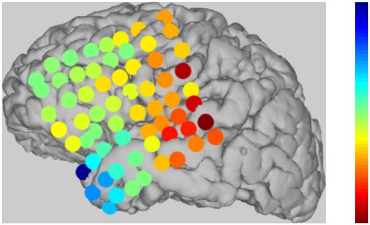
NATURE COMMUNICATIONS | https://doi.org/10.1038/s41467-020-16285-7                                                                            ARTICLE

                             a                                              b
                                                   b               b
                                       a                     a

                                                   c               c

                                           t                     t+1                  t                 t+1               t+2

                             c         Preferred result                    DPPM                 CPM                       MMM
                                                                                                               C2
                             7 edges

                                               t       t+1             t        t+1         t         t+1      C1     t         t+1
                                                                                                               C2
                             8 edges

                                               t       t+1             t        t+1         t         t+1      C1     t         t+1
                                                                                                              C2
                             9 edges

                                               t       t+1             t        t+1         t         t+1     C1      t         t+1

                             d
                                  DPPM
                                  CPM
                                  MMM

Fig. 1 Illustration of DPPM principles and effectiveness. a Schematic of the bridges used to walk plexes within dynamic communities across time. Blue
edges represent inferred connectivity, while red edges connecting the same (solid) or adjacent (dotted) vertices facilitate movement. b Illustrative example
showing how a simple community (in orange) is tracked by DPPM across time in a manner allowing for both coalescence and fragmentation. This
community at first grows at t + 1, and then fragments at t + 2. Another community present at t (purple) perishes at t + 1. c Comparison of DPPM (with 2-
plex of size m = 3, 2nd column), CPM (with 1-plex of size m = 3, 3rd column), and MMM (with γ = 1, ω = 1, 4th column) in determining communities
across two adjacent time points t and t + 1. The connected component at time t + 1 shares increasingly more edges components at time t from the top to
the bottom row of plots. In the preferred results, the dynamic communities (1st column) depend on the number of edges shared from time t to t + 1.
Whereas DPPM treats these as three distinct scenarios, neither CPM nor (effectively) MMM distinguish the three cases. In CPM and MMM, the colorbar
indicates the proportion of community membership over n = 100 repetitions of community detection. d Example dynamic community tracking in the
presence of missing edges. Dynamic community membership for ten example sequential time index networks computed using DPPM (with 2-plex of size
m = 4), CPM (with 1-plex of size m = 3), and MMM (with γ = 1, ω = 1). While DPPM detects a single dynamic community in time, the other two methods
do not.

functional connectivity networks: CPM and MMM19,30. DPPM                                  time t + 1 (Fig. 1c, seven edges). While DPPM detects three
differs from CPM not only in its use of plexes rather than cliques,                       separate communities, both CPM and MMM detect only two
but also in the manner that those are used to define dynamic                               communities. We note that, unlike the deterministic result of
communities. Specifically, CPM only walks the clique within time                           DPPM, the community label at time t + 1 for CPM and MMM is
slices Gt to identify static communities, rather than both within                         not unique. In this example, the community label for CPM at
and across time slices (as in DPPM), using instead a more ad hoc                          time t + 1 is chosen arbitrarily (i.e., by a fair coin flip) from the
rule of overlap among static communities across adjacent times to                         existing community labels at time t37. In the second example, we
form dynamic communities. MMM, in contrast, differs from both                             add an additional edge to the single connected component at time
DPPM and CPM in its core mechanism, adopting an implicit                                  t + 1 (between the upper two nodes, Fig. 1c, eight edges). In this
notion of communities defined via optimization of a cost criterion                         case, DPPM tracks a dynamic community from time t to t + 1
like modularity.                                                                          (red in Fig. 1c, eight edges). While the DPPM result is quite
   To illustrate the impact of these differences, we consider three                       different in this example, the additional edge has little effect on
simple examples of dynamic community tracking between two                                 the dynamic communities detected with CPM and MMM.
sequential networks (Fig. 1c). In the first example, two connected                         Addition of another edge (between the lower two nodes at t +
components at time t evolve to a single connected component at                            1) again changes the DPPM result (Fig. 1c, nine edges); in this

NATURE COMMUNICATIONS | (2020)11:2785 | https://doi.org/10.1038/s41467-020-16285-7 | www.nature.com/naturecommunications                                    3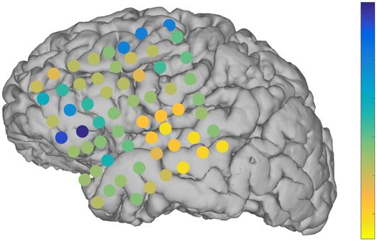
ARTICLE                                                                 NATURE COMMUNICATIONS | https://doi.org/10.1038/s41467-020-16285-7

case, all components at times t and t + 1 establish a single                 see “Methods”). In this illustrative example, only DPPM
community. This occurs because a plex, beginning in the upper                successfully detects the dynamic community contraction with
triangle at time t, can propagate to the single component at time            high sensitivity and specificity (Fig. 3a). Different choices of
t + 1, and then back to the lower triangle at time t. Again, the             module size in CPM, or structural and temporal resolution
addition of an edge has little effect on the dynamic communities             parameters in MMM, tend to detect the dynamic network
detected with CPM and MMM. We note that the choice of MMM                    contraction with low sensitivity, low specificity, or both (Fig. 4b,
parameters γ = 1, ω = 1 serves as a representative example; other            e; see Supplementary Fig. 3 for examples of each community
parameter choices perform similarly (see Supplementary Fig. 1).              detection method applied with different parameter settings).
We conclude that unlike the latter two methods, DPPM                            For the third simulation category, we consider the scenario of
distinguishes between the three subtly distinct basic scenarios in           one community splitting into two. To simulate this scenario, we
an explicit and deterministic way.                                           begin with a single group (see Group A on Fig. 3b, left panel) of
   In addition, we demonstrate the robustness of DPPM to noise.              nodes that share a common community label (see ground truth in
To do so, we begin with a nine-node template network possessing              Fig. 3b, left panel). After an interval of time, two new groups of
eight edges. We then replicate this network 100 times to create a            nodes appear (Groups B and C, Fig. 3b). Each node in these
time-indexed network, such that at each time we remove two                   groups shares a common community label with Group A. All
randomly chosen edges. We expect that a dynamic community                    three groups remain active for an interval of time, establishing a
tracking procedure robust to noise (i.e., type-II errors or missing          dynamic community consisting of nodes from all three groups.
edges) would track a single community in time. We find that                   Then, Group A leaves the common community, while Groups B
DPPM succeeds and successfully tracks a single dynamic                       and C remain in the common community. We expect to detect a
community in time (Fig. 1d, top row), whereas CPM fractures                  single dynamic community splitting from the collection of all
into different transient dynamic community detections (Fig. 1d,              nodes in Groups A, B, and C, to the collection of nodes only in
middle row). While MMM also detects a consistent structure in                Groups B and C (i.e., the blue ground truth community in Fig. 3b,
time, it consists of two dynamics communities, based on the                  left panel).
configuration of the eight edges in the template network (Fig. 1d,               We find that all three methods detect some aspects of the
bottom row). We conclude that edge noise dramatically impacts                dynamic community splitting (Figs. 3b and 4c, e; see Supple-
CPM, while both DPPM and MMM are robust to noise, but only                   mentary Fig. 4 for examples of each community detection method
DPPM detects a single community in time.                                     applied with different parameter settings). However, only DPPM
                                                                             detects the dynamic community splitting with high sensitivity
                                                                             and specificity.
DPPM accurately tracks dynamic communities. To better                           Finally, we consider the converse of splitting: dynamic
characterize the performance of DPPM compared with existing                  community merging. In this scenario, we begin with two groups
dynamic community detection methods, we consider four cate-                  (Groups B and C) whose nodes share a common community label
gories of simulation. Each category simulates a representative               (see ground truth in Fig. 3c, left panel). After an initial interval of
dynamic community behavior, motivated by the notion that brain               time, a third node group (Group A) joins the common
functional networks can expand, contract, split, and merge in                community. Finally, we remove nodes only in Group B and
response to changing task demands, internal states, and disease18.           Group C (Fig. 3c). After these removals, only the Group A nodes
We show that, across these four categories, DPPM outperforms                 share a common community label. We expect to detect a single
existing methods and successfully detects the functional network             dynamic community that begins with nodes in Groups B and C,
community dynamics.                                                          then adds nodes from Group A, and finally consists only of
   We start with simulations of community expansion. The                     Group A nodes. We again find that, although all three methods
simulations begin with a group of nodes that belong to the same              capture some features of the dynamic community merging, only
community (Fig. 2a, b). As time evolves, a second group of nodes             DPPM performs with high sensitivity and specificity (Figs. 3c and
joins the community established by the first group (Fig. 2a, b). At           4d, e; see Supplementary Figs. 5 and 6 for examples of each
a later time, a third group joins the expanding dynamic                      community detection method applied with different parameter
community. In this way, the community expands to encompass                   settings).
larger groups of nodes as time evolves. We note that all nodes that             Based on the results from these four simulation categories
join the expanding group share a common community label,                     (summarized in Fig. 4), we conclude that only DPPM detects the
while nodes outside of this expanding group are assigned a                   dynamic community behavior with high sensitivity and high
random community labels (see “Methods”).                                     specificity in all scenarios considered. We find that no fixed
   Application of the three dynamic community detection                      parameter setting for MMM performs with both high sensitivity
methods yields distinctly different results. While in this example           and high specificity across all simulation scenarios. While DPPM
CPM fails to capture the community expansion, both DPPM and                  and CPM perform with similar specificity across parameter
MMM succeed (Fig. 2c). We note that here, and in the                         settings, DPPM (with m = 4, k = 2; m = 4, k = 3; or m = 5, k = 3)
simulations that follow, we fix the detection method parameters               perform with higher sensitivity than CPM.
to show representative examples; see Supplementary Fig. 2 for
examples of each community detection method applied with
different parameter settings.                                                Expansion of a dynamic community at human seizure onset.
   In the second category of simulation, we consider dynamic                 To illustrate the performance of DPPM on clinical data, we
community contraction, which can intuitively be understood as                consider an application to invasive electrocorticogram (ECOG)
dynamic community expansion with time reversed. For these                    recordings from an 8 × 8 electrode grid placed directly on the
simulations, we begin with a large group of nodes that share a               cortical surface of a human patient undergoing resective surgery
common community label (see ground truth on Fig. 3a, left                    for epilepsy (see “Methods”). From these data, we infer dynamic
panel). As time evolves, we remove nodes from this community.                functional networks (see “Methods”) that begin 100 s before sei-
By doing so, we expect to reduce the number of nodes that                    zure onset, and examine the dynamic communities that emerges
participate in the dynamic community, until eventually all nodes             at seizure onset in four seizures. We choose to examine seizure
are removed (and each node assigned a random community label,                onset, where a rapid increase in functional connectivity often

4                NATURE COMMUNICATIONS | (2020)11:2785 | https://doi.org/10.1038/s41467-020-16285-7 | www.nature.com/naturecommunications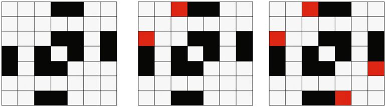
NATURE COMMUNICATIONS | https://doi.org/10.1038/s41467-020-16285-7                                                                                          ARTICLE

                           a             t   [20s, 39s]       t    [40s, 59s]        t     [60s, 79s]         t    [80s, 99s]       t        [100s, 119s]
                                    1

                            Nodes
                                    8
                                         1                8
                                             Nodes

                           b         1
                            Nodes

                                    64
                                         1            64
                                             Nodes

                           c                 True expand                  DPPM                               CPM                             MMM
                                    1                              1                           1                                1
                            Nodes

                                    64                            64                          64                           64
                                             40 80 120                  40      80   120                40    80    120                 40     80   120
                                              Time (s)

Fig. 2 In an example of dynamic community expansion, DPPM outperforms two existing methods. Illustration of community expansion in nodes (a) and
in edges (b). a Two-dimensional representation of the nodes on an 8 × 8 grid at five time intervals. Color (blue) indicates when a node becomes recruited
to the largest community. b Adjacency matrices for the simulated network of 64 nodes at the same five time intervals. Color (black) indicates an edge
between a node pair. c Dynamic community detection results for each method, from left to right: true expansion, DPPM with parameters m = 4 and k = 2,
CPM with parameter m = 4, and MMM with parameters γ = 0.1, ω = 0.1; see Supplementary Figs. 2 and 6a for results with different parameter choices,
and see Fig. 4a, e for average results over 100 realizations of the simulation. Color indicates community membership. The largest community detected by
DPPM is most consistent with the true expansion.

occurs38,39. Before seizure onset, a large number of small dynamic                          join). Visual inspection of the median maps of node recruitment
communities transiently appear (N = 1768 communities detected                               order (Fig. 5g) across the patient’s four seizures suggests
for n = 4 seizures, example in Fig. 5a). The vast majority of these                         recruitment occurs in a spatially organized pattern; neighboring
communities are short-lived (median lifespan 1 s, 95% of life-                              nodes tend to be sequentially recruited in the seizure onset
spans
ARTICLE NATURE COMMUNICATIONS | https://doi.org/10.1038/s41467-020-16285-7
a Group truth DPPM CPM MMM
1 1 1 1
Nodes
64 64 64 64
40 80 120 40 80 120 40 80 120 40 80 120
Time (s)
b 1 1 1 1
B
A
Nodes
C
64 64 64 64
40 80 40 80 40 80 40 80
Time (s)
c 1 1 1 1
B
A
Nodes
C
64 64 64 64
40 80 40 80 40 80 40 80
Time (s)
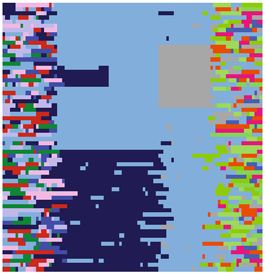
Fig. 3 In three additional examples of dynamic community evolution, DPPM outperforms two existing methods. Community detection for each method
in the case of a community contraction, b community splitting, and c community merging. From left to right in each subfigure: true community evolution,
DPPM with parameters m = 4 and k = 2, CPM with parameter m = 4, and MMM with parameters γ = 0.1, ω = 0.1; see Fig. 4 and Supplementary Figs. 3–6
for results with different parameter choices. Color indicates community membership. In all cases, the largest community detected by DPPM is most
consistent with the true community evolution.
population means [−0.59, −0.04]; and p = 0.0016, t-statistic = expansion at seizure onset from an initial set of nodes, and that
−3.41, 95% confidence interval for the difference in population community structure during seizure correlates with surgical
means [−0.46, −0.11]; respectively, two-tailed two-sample t-test, outcome.
n = 27 from nine patients with low Engel score, and n = 11 from The results presented here may appear to challenge previous
three patients with high Engel score, degrees of freedom = 36). applications of dynamic community evolution procedures to
We conclude from these observations that application of human brain activity21–23,25–27,30,41–44. However, one should not
DPPM to ECOG data recorded from patients with epilepsy dismiss this prior work. We showed in simulation that MMM
provides new insights into the expansion of a large dynamic may still produce accurate results, and the ability to investigate a
community at seizure onset. We propose that larger communities range of resolution parameter values may provide a more com-
of longer duration emerge during seizure, and that patients with prehensive view of a network’s modular organization45. Different
fewer, shorter duration communities during seizure have brain activity (e.g., slow hemodynamic responses versus fast
improved surgical outcomes. electrophysiological changes) may results in dynamic functional
networks more compatible with accurate inference over a broad
Discussion range of resolution parameters. While DPPM only links nodes at
In this manuscript, we introduced the DPPM to track dynamic neighboring time steps, MMM permits links between nodes
communities that evolve in time. We designed this method spe- across broader time intervals. Such links may support more
cifically to address the challenges introduced when inferring accurate detection of communities in which nodes infrequently—
dynamic functional networks from neural time series data. The but consistently—participate. We note that the communities
resulting method differs from existing dynamic community identified by any method, while not necessarily optimal, could
tracking procedures in two ways. First, we extract communities still facilitate fruitful exploration of functional brain networks.
based on the explicit notion of time-evolving aggregations of For example, the distinction between a large community, and two
smaller motifs, rather than through optimization of a cost cri- smaller communities that evolve similarly, may not have practical
terion. Second, we account for edge noise—a factor in any set of consequences to understanding brain function or dysfunction.
functional networks inferred from time series data. We showed in While DPPM performs well in simulations, and in an example
simulations that DPPM outperforms two existing methods in application to in vivo data, we note three limitations. First, the
representative dynamic network scenarios motivated by the computational time required to track dynamic networks with
intuitive notions of community expansion, contraction, merging, DPPM depends on the plex size, and hence is likely to be most
and splitting. We then applied DPPM to examples of time- practical for plexes of relatively small scale. We developed
indexed functional networks inferred at human seizure onset. We approximations to reduce computational time in two cases—(4,2)
showed preliminary evidence of rapid, dynamic community and (5,3)—which are consistent with the size of structural and
6 NATURE COMMUNICATIONS | (2020)11:2785 | https://doi.org/10.1038/s41467-020-16285-7 | www.nature.com/naturecommunications
NATURE COMMUNICATIONS | https://doi.org/10.1038/s41467-020-16285-7 ARTICLE
a Expansion b Contraction c Splitting d Merging
1 1 1 1
0.8 0.8 0.8 0.8
Specificity
Specificity
Specificity
Specificity
0.6 0.6 0.6 0.6
0.4 0.4 0.4 0.4
0.2 0.2 0.2 0.2
0 0 0 0
0 0.2 0.4 0.6 0.8 1 0 0.2 0.4 0.6 0.8 1 0 0.2 0.4 0.6 0.8 1 0 0.2 0.4 0.6 0.8 1
Sensitivity Sensitivity Sensitivity Sensitivity
e
Expansion
1
Specificity
0.5
0
1
Sensitivity
0.5
0
Contraction
1
Specificity
0.5
0
1
Sensitivity
0.5
0
Splitting
1
Specificity
0.5
0
1
Sensitivity
0.5
0
Merging
1
Specificity
0.5
0
1
Sensitivity
0.5
0
DPP(4,1)
DPP(4,2)
DPP(4,3)
DPP(5,1)
DPP(5,2)
DPP(5,3)
CPM(3)
CPM(4)
CPM(5)
CPM(6)
MMM(2,10)
MMM(2,5)
MMM(2,2)
MMM(2,1)
MMM(2,0.5)
MMM(2,0.1)
MMM(2,0.01)
MMM(1,10)
MMM(1,5)
MMM(1,2)
MMM(1,1)
MMM(1,0.5)
MMM(1,0.1)
MMM(1,0.01)
MMM(0.5,10)
MMM(0.5,5)
MMM(0.5,2)
MMM(0.5,1)
MMM(0.5,0.5)
MMM(0.5,0.1)
MMM(0.5,0.01)
MMM(0.1,10)
MMM(0.1,5)
MMM(0.1,2)
MMM(0.1,1)
MMM(0.1,0.5)
MMM(0.1,0.1)
MMM(0.1,0.01)
MMM(0.01,10)
MMM(0.01,5)
MMM(0.01,2)
MMM(0.01,1)
MMM(0.01,0.5)
MMM(0.01,0.1)
Fig. 4 DPPM performs with higher sensitivity and specificity than two existing methods in the four simulation scenarios. Specificity and sensitivity of
DPPM (blue), CPM (red), and MMM (yellow) for n = 100 independent simulations with different noise instantiations of each dynamic community
evolution scenario. a Community expansion, b Community contraction, c Community splitting, and d Community merging. Each circle indicates the result
of one simulation with one parameter configuration (see “Methods”). e Summary results for each community tracking method applied to each simulation
scenarios. Bars indicate the mean sensitivity and specificity for each parameter configuration of each method. Dots indicate the results of the n = 100
simulations for each simulation scenario and method.
functional motifs proposed as common network building blocks of the brain46, motifs may instead represent a byproduct of
blocks31,32. DPPM successfully aggregates these common motifs local brain connectivity47,48. The connection of DPPM with
into communities. We note that the appropriate interpretation of motifs through the central role of plexes may facilitate more
network motifs in neuroscience remains a point of open discus- explicit study of this issue going forward, in the specific context of
sion. While motifs have been proposed as network building dynamic community detection. Applications to different systems,
NATURE COMMUNICATIONS | (2020)11:2785 | https://doi.org/10.1038/s41467-020-16285-7 | www.nature.com/naturecommunications 7
ARTICLE NATURE COMMUNICATIONS | https://doi.org/10.1038/s41467-020-16285-7
a
Node subset
10
20
Nodes
30
40
50
60
Size of the biggest community
60
50
40
30
20
10
0
–100 –90 –80 –70 –60 –50 –40 –30 –20 –10 0 10 20 30 40 50 60
Time (s)
b
c e f
103
65
100
Community count
102 75 55
Loyalty (s)
Loyalty (s)
50
10 45
25
1 35
1 50 100 200
Community lifespan (s)
d g h
103
12 14
Mean recruitment time (s)
Median expanding order
Community count
10 12
102 10
8
8
6 6
10
4 4
2
1 2
1 10 20 30 40 50 60 0
Maximum community size
i j k 2 l 1
duration (normalized)
Longest community
Number of seizures
Number of seizures
30 30
of communities
Mean number
20 20
1
10 10
0 0 0 0
0 0.2 0.4 0.6 0.8 1 0 0.2 0.4 0.6 0.8 1 Engel 1,2 Engel 3,4 Engel 1,2 Engel 3,4
Maximum community size Maximum community lifespan
(normalized) (normalized)
in which larger plexes are required, may require additional Second, DPPM may link dynamic communities which may be
development. Along this line, maximal k-plex identification, interpreted as separate based on information beyond the network
which is a computationally costly algorithm at the core of DPPM, connectivity. To illustrate this, we consider the hypothetical
has received renewed interest in network sciences, which could scenario in which two dynamic communities exist simulta-
lead to further speed improvements49,50. neously. Within one community, a low frequency rhythm (e.g.,
8 NATURE COMMUNICATIONS | (2020)11:2785 | https://doi.org/10.1038/s41467-020-16285-7 | www.nature.com/naturecommunications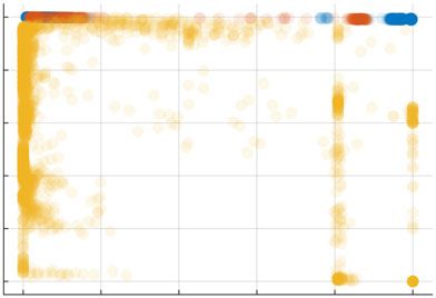
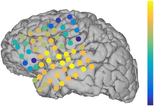
NATURE COMMUNICATIONS | https://doi.org/10.1038/s41467-020-16285-7                                                                         ARTICLE

Fig. 5 Application of DPPM reveals new characteristics of dynamic communities before and after human seizure onset. a Top: Voltage time series
recorded at nine electrodes to illustrate pre-seizure and seizure voltage dynamics. Middle: Example recruitment of a large community at seizure onset.
Before seizure onset (t < 0 s) small communities appear briefly; color indicates community membership. After seizure onset (t > 0 s) a large dynamic
community appears (red) that persists for over 30 s. Bottom: Temporal evolution of the size of the seizure onset community (red). Nearly all nodes
participate in the seizure onset community. b Example expansion of the seizure onset community. Each circle denotes an electrode on the 8 × 8 electrode
grid, and red (black) indicates electrodes recruited (not yet recruited) into the dynamic community. Community lifespan (c) and maximum community size
(d) for all pre-seizure communities (gray histograms) and the seizure onset community observed for each of the four seizures of this patient (four arrows,
red indicates the community shown in (a)). Node loyalty averaged over the four seizures for (e) all pre-seizure communities and (f) the seizure onset
community. In both panels, warm (cool) colors indicate nodes that participate in communities for longer (shorter) times. The black circles indicate a subset
of electrodes that have high node loyalty before and during early seizure. g Median recruitment order to the seizure onset community for four seizures.
Warm (cool) colors indicate electrodes recruited earlier (later) into the seizure onset community. h Mean recruitment time to large amplitude ictal
oscillations observed for the same patient, as reported in ref. 65. Warm (cool) colors indicate electrodes recruited earlier (later) into ictal spread.
Histograms of the size (i) and the lifespan (j) of the maximum community during the pre-seizure (blue) and seizure (red) intervals from each patient and
seizure. The maximal community tends to be larger and of longer duration during seizure. The mean number of communities (k) and the longest
community duration (l) during seizure for patients with good (Engel 1,2) and poor (Engel 3,4) surgical outcomes. Each circle indicates an individual seizure,
and the red square the population mean (n = 27 from nine patients with low Engel score, and n = 11 from three patients with high Engel score). Worse
surgical outcomes exhibit more communities with longer maximal duration during seizure.

theta, 4–8 Hz) links the nodes, while in the other dynamic                      connectivity may lead to different inferred functional networks
community, a higher frequency rhythm (e.g., beta, 12–20 Hz)                     and different dynamic communities. How this uncertainty
links the nodes. Initially, because different frequency rhythms                 impacts the standard tools of network analysis remains poorly
appear in each community, no links exist between the two                        understood. Moreover, these inferred—and uncertain—func-
communities; i.e., the communities are functionally disconnected.               tional networks change rapidly in time43,55,56. Finding the best
Then, at a later time, nodes in both communities transition to the              approaches to infer and characterize dynamic communities from
same rhythm (e.g., alpha, 8–12 Hz), establishing functional con-                noisy, non-stationary brain signals is a significant challenge. We
nections between the nodes in both communities, and causing the                 note that the appropriate choice of plex could change as a
two dynamic communities to merge. In this scenario, DPPM                        function of time. How, why, and the extent to which this would
would identify a single dynamic community that includes all                     be can be expected to vary with context. However, at a minimum,
nodes at all time considered. That the two sets of nodes initially              nontrivial changes in network density over time can be expected
form separate functional communities—employing rhythms in                       to be a factor. In the context of epilepsy, it has been observed that
different frequency bands—is not represented in the single                      network density can evolve dramatically during a seizure34. This
dynamic community identified by DPPM. Analysis of node                           might suggest the value of developing an extension of DDPM (as
properties (e.g., the power spectrum) or selection of coupling                  well as related methods like CPM) with adaptively chosen, time-
measures targeting specific frequency bands would address this                   varying plex order.
particular scenario.                                                               In this manuscript, we considered a systematic comparison of
   Third, DPPM is designed for binary networks that are often                   DPPM with two representative methods, CPM and MMM, as
inferred from multi-electrode brain recordings, but in neu-                     implemented in the literature. However, we note that modifica-
roscience it is frequently desirable to analyze weighted networks.              tions of these methods—by interchanging characteristics of
CPM has been extended to weighted networks51, where in order                    DPPM, CPM, and/or MMM—would allow a more comprehen-
to percolate cliques are now required to be of sufficient intensity              sive exploration of the benefits and contributions of specific
(i.e., the geometric mean of the link weights in a clique52 must                method characteristics to dynamic community detection in gen-
exceed a given threshold). An extension of DPPM to weighted                     eral. For example, in DPPM we link networks in time by
networks should be similarly feasible, although somewhat less                   including an edge from each node to itself, and to all other nodes
immediate for two reasons. First, there can be a multiplicity of                with which it shares consistent connections (Fig. 1a). This is a
plexes among a given set of nodes, and thus there is flexibility in              generalization of the coupling usually used in MMM; extending
representation. One approach might be to adopt the recently-                    MMM to link networks in time as in DPPM would help reveal the
introduced notion of a maximal edge-weighted plex53. Second, it                 impact of this specific method characteristic. In DPPM, the cross-
is necessary to equip the edges between the same nodes at dif-                  network links proposed have a simple and explicit approach. This
ferent network time points with an appropriate notion of an edge                approach, for connecting nodes to themselves across time, is
weight. Depending on the manner of network construction, there                  implicitly a local smoothing of the network structure itself, with
may be multiple ways in which to do so. A full and careful                      the degree of smoothing connected to the choice of plex k. An
exploration of these possibilities is beyond the scope of the pre-              alternative approach to link networks in time is a temporal
sent manuscript. We note that MMM handles weighted edges                        smoothing of network connectivity matrices across adjacent
seamlessly and without modification.                                             frames. While this approach would link networks in time using all
   While tools from network analysis serve an essential role in                 connections, it would also introduce a new smoothing parameter;
understanding multisensor recordings54, significant challenges                   how to best choose this smoothing parameter automatically is not
remain in the application of these tools. In social networks or                 clear. While we explored a wide range of method variations here,
association networks, for which many network tools were                         additional modifications may allow CPM and MMM to perform
developed, the edges are known with certainty (e.g., social                     similarly to DPPM (e.g., the choice of null model in MMM, or an
network friends or manuscript co-authors). However, in func-                    alternative procedure to couple networks across layers in CPM).
tional networks inferred from noisy brain activity, the edges are               However, such extensions are beyond the scope of the present
estimated with uncertainty. This uncertainty depends—in com-                    manuscript.
plex ways—on the association measure applied and the nature of                     Understanding the brain’s network dynamics remains a fun-
the data recorded. Different measures to define functional                       damental challenge in neuroscience, with opportunities spanning

NATURE COMMUNICATIONS | (2020)11:2785 | https://doi.org/10.1038/s41467-020-16285-7 | www.nature.com/naturecommunications                                   9
ARTICLE                                                                                       NATURE COMMUNICATIONS | https://doi.org/10.1038/s41467-020-16285-7

from genetic networks to social networks57, and applications                                        algorithm for identifying maximal k-plexes in a graph has time complexity that is
spanning health and disease. Here we focus on one component of                                      output sensitive and performs, experimentally, as sub-exponential.
                                                                                                        In practice, several steps are taken to increase computational efficiency. Within
this challenge: the characterization of dynamic communities in                                      StatComm the secondary graph G* is never explicitly constructed. Rather, we
evolving functional connectivity networks, and application to the                                   simply compute the overlap between all pairs of k-plexes and determine
dynamic networks that emerge during human seizures. While                                           community labels accordingly. We use a threshold of (m − 1) when considering the
characterization of seizure onset requires inference and analysis                                   vertex overlap between k-plexes to build the plex graph and find its connected
of rapidly evolving functional networks, we expect the dynamic                                      components. Finally, to avoid having to build a 2p × 2p adjacency matrix from each
                                                                                                    of the enhanced multi-slice graphs Gþ   t we employ a strategy that has been shown
community tracking approach developed here will apply to other,                                     (using exhaustive enumeration) to be almost exact for DPPM parameters up to
multivariate neuronal data sets (e.g., calcium imaging, MEG,                                        (5,3). Specifically, our heuristic measures the overlap between all pairs of
multi-neuron recordings). Ultimately, the continued development                                     communities found at time steps t and t + 1 and labels them as the same
of statistically principled network analysis tools—combined with                                    community if the overlap is greater than m − 1 vertices. This approach is almost
                                                                                                    exact in the sense that, when applying DPPM for plexes of size m, it reproduces the
advances in data acquisition and computational modeling—is                                          results of the formal algorithm (i.e., based on the exact rule walking across time
essential to understanding the neural origin, mechanisms, and                                       slices) except that when encountering an m-cycle, which is matched with its
functions of the brain’s dynamic functional connectivity.                                           isomorphic motifs (e.g., hourglass to square and vice-versa for size 4). We do not
                                                                                                    expect this approximation to impact the network communities of interest here for
                                                                                                    two reasons. First, cycle and isomorphic motifs are unlikely due to transitive
                                                                                                    connections common in correlation networks59. Second, the size of the
Methods                                                                                             communities we observe typically exceeds 4 or 5 nodes, so that alternative plexes
DPPM. The DPPM identifies all dynamic subgraphs over which a k-plex of at least                      could stitch the communities in time. We view these trade-offs as acceptable when
order m vertices can be ‘walked’. From an algorithmic standpoint, DPPM consists                     held against the significant computational improvements the approximation brings
of three subroutines: Plex, StatComm, and DynComm. We briefly describe these                         when applied to the functional networks of interest here. We find that, in practice,
subroutines and their implementation here; pseudo-code versions can be found                        DPPM tends to run in less time than MMM and CPM (Supplementary Fig. 7).
in Supplemental Materials.
    Given an input graph on p vertices, say G = (V,E), Plex identifies the maximal
k-plexes, based on ref. 58. That is, all vertex-induced subgraphs S1, S2,… are                      Existing dynamic community detection methods. In addition to DPPM, we
enumerated such that each Sj is a k-plex of size nj and, if any other vertex is added               apply two other dynamic community detection methods already in existence. We
to Sj, it would cease to be a plex. In practice, since a clique is also a k-plex and                implement MMM following the procedure described in ref. 19 and using the
finding a clique is faster, we start by finding all maximal cliques larger than m and                 MATLAB code (including the GenLouvain function) available at http://netwiki.
then look for k-plexes within the remaining vertices that are not parts of any                      amath.unc.edu/GenLouvain/GenLouvain, Version 2.1. An additional post-
cliques.                                                                                            processing step was applied to refine the results: we discard identified communities
    Using Plex, StatComm effectively creates from an input graph G a secondary                      that are deemed too small (here, size strictly lower than 3) and too short-lived (only
graph G*, with each vertex corresponding to a maximal k-plex Sj in G. An edge                       found for one time step). We implement CPM following the procedure described
exists between two vertices i and j in G* if the number of vertices common to Si                    in18 and using in-house MATLAB code available at the repository associated with
and Sj is at least m − 1 vertices, indicating that a k-plex Si may be walked to the k-              this paper (see “Code availability”).
plex Sj. This step is similar to the CPM that requires a minimum overlap of m − 1                       To estimate the dynamic communities in MMM requires optimization of a
vertices to aggregate cliques into communities18. The connected components in                       quality function with respect to a chosen null model. Different choices exist60,
G*, say C1* ; C2* ; ¼ , then implicitly represent subsets of vertices/edges in the                  including approaches that account for functional networks (i.e., networks derived
                                                                                                    from time series data30), which may alter features of the dynamic communities
original input graph G over which a k-plex may be walked. These vertices/edges are
                                                                                                    detected (e.g., the number and size of communities). Here we choose the standard
assigned labels according to their membership in these connected components. A
                                                                                                    null model (the Newman–Girvan null model), which may detect fewer
vertex/edge may have multiple labels.
                                                                                                    communities of larger size than other approaches30. While this choice of null
    Ultimately, DPPM consists of applying StatComm in two passes through a
                                                                                                    model is common in analysis of neural data21,23,25,26,41, alternative choices (e.g.,
dynamic network fGt gNt¼1 . Recall that the vertex sets Vt in each graph Gt are                     Erdős–Rényi) tailored to specific applications may enhance performance. In
assumed to be equal to a common set V of p vertices. In the first pass, StatComm is                  addition, we note that in practice examination of dynamic functional brain
first applied at each time slice t to determine the static communities within each Gt.               networks requires a comparison of the extracted statistics (such as the module
In the second pass, StatComm is applied to each of N − 1 enhanced multi-slice                       allegiance, flexibility, or laterality) to those expected in a random network null
graphs with 2p vertices containing pairs of graphs adjacent in time. Each new                       model30. This can be done with post-optimization null models, for which different
multi-slice graph, say Gþ      t consists of copies of Gt and Gt+1, wherein a vertex i is           choices exist (e.g., temporal, nodal, and static)30. Because we know the true
labeled vti for its copy from Gt and vtþ1   i
                                                 for its copy from Gt+1. Next, we enhance           network structure in the simulated data, we did not examine such post-
this new graph Gþ                                                 i
                       t by adding an edge between vertices vt and their matured self               optimization null models here.
vtþ1 . We also add edges between (vt , vtþ1 ) and (vtþ1 , vt ) to Gþ
  i                                       i    j          i     j              i j
                                                                       t if (vt , vt ) is an edge
                                                                                                        While the focus of our work here is specifically motivated by the problem of
              i
in Gt and (vtþ1
                     j
                  , vtþ1 ) is an edge in Gt + 1. This provides a means for the community            characterizing the evolution of functional connectivity networks during epileptic
                                                                                                    seizures, and the details and design choices underlying the proposed DPPM derive
to walk across time, and visually appears as what we term railroad tracks in Gþ            t (see   directly therefrom, there is of course a large and active literature on dynamic
Fig. 1a). Community labels associated with vertices/edges within each of the slices
                                                                                                    community detection in general. The recent survey by Rosetti and Cazabet33 offers
Gt from the first pass of StatComm are then propagated forward and backward in
                                                                                                    a concise summary of the literature to date, organized according to a certain
time through the resulting augmented dynamic graph fGþ                 N
                                                                    t gt¼1 , in an iterative        taxonomy (see their Fig. 4), with the three main classes of instant-optimal
fashion, thus equipping each dynamic community with a unique label.                                 communities discovery, temporal trade-off community discovery, and cross-times
    The computational complexity of DPPM is dominated by the identification of                       communities discovery. In the language of that paper, DPPM is of the third type,
all maximal k-plexes in the Plex algorithm, which in turn is called in the context of               specifically of the sub-type evolving memberships, evolving properties. CPM, in
identifying communities across adjacent time points t and t + 1 using the StatCom                   contrast, is a method primarily of the first type but arguably with some
algorithm. We use a modification of the Bron–Kerbosch (BK) algorithm58, which is                     characteristics of the second type. Finally, MMM is of the third type. The choice of
a recursive backtracking procedure for identifying all maximal cliques in an                        these two algorithms as competitors in our numerical work is therefore
undirected graph consisting of p vertices. Because there are at least as many k-                    representative in the sense that MMM allows for comparison within the same class
plexes as maximal cliques on m vertices,       the worst-case complexity for                      as DPPM, while CPM allows for comparison across the classes. However, it would
                                               p
identification of k-plexes is at least O 33 . Suppose that mt and mt+1 maximal k-                    be of independent interest—although beyond the scope of the current paper—to
plexes are returned by the algorithm on the graphs Gt and Gt +1, respectively. The                  evaluate the performance of DPPM broadly, against many methods and on a large
static communities at times t  and t+ 1 are determined  by comparing the sizes of                compendium of networks.

                                  mt         mtþ1
vertex set intersections of all         þ           pairs of k-plexes within time
                                   2           2                                                    Patients and recordings. The patient analyzed in Fig. 5a–h was a 37-year-old male
slices. Similarly, the dynamic communities between times t and t + 1 are                            with medically intractable focal epilepsy who underwent clinically indicated
determined by comparing the sizes of vertex set intersections of all mtmt+1 pairs of                intracranial cortical recordings using grid electrodes for epilepsy monitoring.
k-plexes across time slices. Let dt be the number of vertices in the largest maximal                Clinical electrode implantation, positioning, duration of recordings and medication
k-plex in time slice t, and d = max(dt, dt+1). Then each pairwise comparison is O                   schedules were based purely on clinical need as judged by an independent team of
(dlogd) complexity using a standard merge sort. Subsequently, breadth-first-search                   physicians. The patient was implanted with intracranial subdural grids, strips, and
determines the connected components in O(mt + mt+1) time. In total, letting m =                     depth electrodes (Adtech Medical Instrument Corporation) for 10 days in a spe-
max(mt,mt+1), identifying communities from time t to t + 1 has a worst-case                         cialized hospital setting and continuous ECOG data were recorded (500 Hz sam-
complexity of at least O(dlogdm2). Empirical results indicate that our modified BK                   pling rate). The reference was a strip of electrodes placed outside the dura and

10                      NATURE COMMUNICATIONS | (2020)11:2785 | https://doi.org/10.1038/s41467-020-16285-7 | www.nature.com/naturecommunications
NATURE COMMUNICATIONS | https://doi.org/10.1038/s41467-020-16285-7 ARTICLE
facing the skull at a region remote from the other grid and strip electrodes. One to Split: splitting of one community into two communities. In this scenario, we
four electrodes were selected from this reference strip and connected to the simulate three dynamic communities c1, c2 and c3. Each consists of 15 nodes. We
reference channel. divide the timeline of this scenario into 5 intervals of duration 20 s each, as follows
Seizure onset times were determined by an experienced encephalographer (Fig. 3b):
(S.S.C.) through inspection of the ECOG recordings, referral to the clinical report,
and clinical manifestations recorded on video. We selected four seizures to analyze (1) Initially each node is assigned a random community label (a randomly
for this patient. Their durations were respectively 75.94 s, 62.79 s, 60.14 s, 133.16 s. chosen integer between 1 and 64) for each layer (i.e., 1 s) of the 20 s interval.
We included 100 s before seizure onset in each dataset. No dynamic communities exist.
The population of patients analyzed in Fig. 5i–l corresponds to patients P1–P6, (2) Only community c2 is active; each node receives the same community label.
P9, P11, P12, P13, P15, and P16 in Table 1 of ref. 40. We note that, in comparing (3) Communities c1 and c3 become active; each node receives the same
patients with different surgical outcomes (Fig. 5k, l), we treat multiple seizures community label as c2.
from the same patients as independent. (4) Community c2 becomes inactive (each node receives a random community
All human subjects were enrolled after informed consent was obtained and label), and only communities c1 and c3 remain.
approval was granted by local Institutional Review Boards at Massachusetts (5) Communities c1 and c3 become inactive; all nodes receive a random
General Hospital and at Boston University according to National Institutes of community label, as in (1).
Health guidelines.
Merge: merging of two communities into one community. Conceptually, this
simulation is the converse of the split scenario. We again simulate three dynamic
Deterministic community detection simulation. We consider two networks,
communities c1, c2 and c3, each consisting of 15 nodes. We divide the timeline of
each of seven nodes. The first network, which exists at time t, consists of six
this scenario into 5 intervals of duration 20 s each, as follows (Fig. 3c):
edges organized in the adjacency matrix plotted in Fig. 6a. For the second
network, which exists at time t + 1, we consider the three alternative adjacency (1) Initially no communities are active; each node is assigned a random
matrices plotted in Fig. 6b. The 7-, 8-, and 9-edge networks correspond to community label (a randomly chosen integer between 1 and 64) for each
Fig. 1c top, middle, and bottom row of plots, respectively. We apply each layer (i.e., 1 s) of the 20 s interval.
community detection method to the sequence of two networks: (1) the (2) Communities c1 and c3 become active (each node receives the same
network at time t, and (2) one of the networks selected at time t + 1. community label), without any nodes in common.
Because the CPM and MMM do not provide deterministic community (3) Community c2 becomes active, and receives the same community label as c1
assignments, we repeat each method 100 times on the two-network sequence, and c3.
and indicate the proportion of times each node is assigned to one (of two) (4) Communities c1 and c3 become inactive (each node is assigned a random
communities. community label), and only c2 remains.
(5) Communities c2 becomes inactive; all nodes receive a random community
label, as in (1).
Robustness to noise simulation. To illustrate how the three dynamic community
detection methods perform when functional network inference is corrupted by
false negatives (i.e., missed edges) we perform the following simulation. We begin Expand: one community expands. In this simulation, we simulate five commu-
with a connected nine-node network with adjacency matrix plotted in Fig. 6c. We nities c1, …, c5. We divide the timeline of this scenario into seven equal intervals
then simulate a dynamic network for 100 time steps, by removing two edges chosen (20 s duration), such that in each interval we add additional nodes to the com-
at random from the adjacency matrix at each time step. We apply each community munity, as follows (Fig. 2):
detection method to the resulting sequence of 100 networks.
(1) Initially each node is assigned a random community label (a randomly
chosen integer between 1 and 64) for each layer (i.e., 1 s) of the 20 s interval.
During this interval, no organized community structure exists.
Dynamic network simulations. We construct simulated network data motivated
(2) Community c1 with 15 nodes becomes active; each node receives the same
by multi-electrode brain voltage recordings. To do so we consider a 64-electrode
community label.
recording, and generate benchmark dynamic network models using the algorithm
(3) Community c2 with 10 nodes becomes active; each node receives the same
defined in ref. 61 and available at https://github.com/MultilayerGM/MultilayerGM-
community label as c1.
MATLAB, Version 1.0.1. For each simulation scenario, we implement a multilayer
(4) Community c3 with 10 nodes becomes active, and each node receives the
partition (S) with 64 nodes and either 100 time points (Split, Merge) or 140 time
same community label as c1 and c2.
points (Expand, Contract), as described in the following subsections. For con-
(5,6) We continue to add communities in each interval (i.e., community ck with
creteness, we assume each layer of the multilayer network represents a functional
10 nodes becomes active) until all 5 communities have been recruited.
network inferred for a 1 s interval; i.e., the total duration of a simulated dynamic
(7) All communities become inactive; all nodes receive a random community
networks is either 100 s (Split, Merge) or 140 s (Expand, Contract). For each
label, as in (1).
community detection method and for each parameter set investigated for this
method, we repeat each simulation scenario 100 times, with different realizations of
the multilayer partition S. The parameter sets evaluated for each method are as
Contract: one community contracts. Conceptually, this simulation is the converse
follows: DPPM (m,k) = (4,1), (4,2), (4,3), (5,1), (5,2) and (5,3); CPM minimum
of the scenario Expand. In practice, we implement this scenario, by first performing
clique size of 3, 4, and 5; MMM all combinations of γ = {0.01,0.1,0.5,1,2}, ω =
all of the steps in the Expand simulation. We then reverse the indexing of the time
{0.01,0.1,0.5,1,2,5,10}.
axis for all nodes (i.e., the last instance of activity in the Expand simulation
becomes the first instance of activity in the Contract simulation). Doing so results
in the following intervals of activity (Fig. 3a):
Simulation scenarios. In each simulation scenario we define a multilayer partition S
to create dynamic communities that evolve in time. To compute the adjacency (1) Initially all communities are inactive; all nodes receive a random community
matrices for each layer, we fix the parameters in ref. 61 as follows: exponent for the label.
power law degree distribution of −2, minimum degree of 3, maximum degree of 20, (2) All communities (c1, …, c5) are active.
mixing parameter of 0, maximum number of rejections for a single block of 100. (3) Community c5 becomes inactive.
a b c
7 edges 8 edges 9 edges
Fig. 6 Illustration of simple simulated networks. Adjacency matrices in which black at coordinate (i, j) indicates an edge from node i to node j. a Seven
node network at time t. b Seven node networks at time t + 1, with 7, 8, and 9 edges. Red indicates edges added to the leftmost network. c Nine node
network.
NATURE COMMUNICATIONS | (2020)11:2785 | https://doi.org/10.1038/s41467-020-16285-7 | www.nature.com/naturecommunications 11You can also read