The high-frequency response correction of eddy covariance fluxes - Part 2: An experimental approach for analysing noisy measurements of small fluxes
←
→
Page content transcription
If your browser does not render page correctly, please read the page content below
Atmos. Meas. Tech., 14, 5089–5106, 2021
https://doi.org/10.5194/amt-14-5089-2021
© Author(s) 2021. This work is distributed under
the Creative Commons Attribution 4.0 License.

The high-frequency response correction of eddy covariance fluxes –
Part 2: An experimental approach for analysing noisy
measurements of small fluxes
Toprak Aslan1 , Olli Peltola2 , Andreas Ibrom3 , Eiko Nemitz4 , Üllar Rannik1 , and Ivan Mammarella1
1 Institutefor Atmospheric and Earth System Research (INAR)/Physics, Faculty of Science, University of Helsinki,
P.O. Box 68, 00014 Helsinki, Finland
2 Climate Research Programme, Finnish Meteorological Institute, P.O. Box 503, 00101 Helsinki, Finland
3 Dept. of Environmental Engineering, Technical University of Denmark (DTU), Lyngby, Denmark
4 Edinburgh Research Station, UK Centre for Ecology and Hydrology (UKCEH), Bush Estate, Penicuik EH26 0QB, UK

Correspondence: Toprak Aslan (toprak.aslan@helsinki.fi)

Received: 4 December 2020 – Discussion started: 23 December 2020
Revised: 7 April 2021 – Accepted: 29 April 2021 – Published: 28 July 2021

Abstract. Fluxes measured with the eddy covariance (EC)             time constant when low-pass filtering is low, whilst the new
technique are subject to flux losses at high frequencies (low-      PSAA21 and CSA√H ,sync successfully estimate the expected
pass filtering). If not properly corrected for, these result in     time constant regardless of the degree of attenuation and
systematically biased ecosystem–atmosphere gas exchange             SNR. We further examine the effect of the time constant ob-
estimates. This loss is corrected using the system’s transfer       tained with the different implementations of PSA and CSA
function which can be estimated with either theoretical or ex-      on cumulative fluxes using estimated time constants in fre-
perimental approaches. In the experimental approach, com-           quency response correction. For our example time series,
monly used for closed-path EC systems, the low-pass filter          the fluxes corrected using time constants derived by PSAI07
transfer function (H ) can be derived from the comparison of        show a bias between 0.1 % and 1.4 %. PSAA21 showed al-
either (i) the measured power spectra of sonic temperature          most no bias, while CSA√H ,sync showed bias of ±0.4 %. The
and the target gas mixing ratio or (ii) the cospectra of both       accuracies of both PSA and CSA methods were not signif-
entities with vertical wind speed. In this study, we compare        icantly affected by SNR level, instilling confidence in EC
the power spectral approach (PSA) and cospectral approach           flux measurements and data processing in set-ups with low
(CSA) in the calculation of H for a range of attenuation lev-       SNR. Overall we show that, when using power spectra for the
els and signal-to-noise ratios (SNRs). For a systematic anal-       empirical estimation of parameters of H for closed-path EC
ysis, we artificially generate a representative dataset from        systems the new PSAA21 outperforms PSAI07 , while when
sonic temperature (T ) by attenuating it with a first order fil-    using cospectra the CSA√H ,sync approach provides accurate
ter and contaminating it with white noise, resulting in various     results. These findings are independent of the SNR value and
combinations of time constants and SNRs. For PSA, we use            attenuation level.
two methods to account for the noise in the spectra: the first is
the one introduced by Ibrom et al. (2007a) (PSAI07 ), in which
the noise and H are fitted in different frequency ranges, and       1   Introduction
the noise is removed before estimating H . The second is
a novel approach that uses the full power spectrum to fit           Vertical turbulent fluxes of momentum, energy, and gases be-
both H and noise simultaneously (PSAA21 ). For CSA, we              tween the atmosphere and the biosphere measured by the
use a method utilizing the square root of the H with shifted        eddy covariance (EC) technique are subject to both low- and
vertical wind velocity time series via cross-covariance max-        high-frequency losses (Foken, 2008; Aubinet et al., 2012).
imization (CSA√H ,sync ). PSAI07 tends to overestimate the          The physical limitations in instrument response times, spa-

Published by Copernicus Publications on behalf of the European Geosciences Union.
5090                                                                T. Aslan et al.: The choice of the spectral correction method

tial separation of instruments, line averaging, and air trans-        sensor separation. In this approach, the effect of sensor sepa-
port through the sampling tubes cause high-frequency losses           ration is then treated explicitly with an additional correction
(Aubinet et al., 1999).                                               step (Horst and Lenschow, 2009). In most cases the instru-
   The EC sampling system acts as a low-pass filter on the            mental noise becomes visible in the high-frequency range of
flux, and the signal loss must be compensated for with the            χ 0 power spectra, and this has to be dealt with before the time
frequency response correction (FRC) during post-processing.           constant of the gas sampling system can be estimated. The
The first step in the FRC is the description of the effect of the     noise removal procedure is not well established, and this rep-
low-pass filtering of the measurement system, and for this,           resents a major uncertainty in the PSA approach. This paper
the transfer function approach has been widely used since it          explores this uncertainty and proposes a novel, more robust
was first proposed by Moore (1986). The joint transfer func-          approach to account for the noise in PSA.
tion (H ) that describes the low-pass filtering of the whole             On the other hand, this noise is often assumed not to cor-
EC system can be determined theoretically or experimentally           relate with the fluctuations in w, and therefore it does not
(Foken, 2008; Aubinet et al., 2012). The theoretical approach         contribute to the cospectra between w and χ. If this holds,
involves various specific transfer functions that are estimated       this makes the CSA attractive for the estimation of the time
to represent different causes of flux loss. Conversely, in the        constant because then the noise would effectively disappear
experimental approach H is estimated from in situ measure-            from the measured signal. Yet, the use of the CSA relies on
ments. Due to its simplicity, many studies have implemented           the correct determination of the time lag between w and χ ,
the theoretical approach, which typically works well with             which may be difficult in the case of small fluxes due to nois-
fluxes measured by open-path EC systems, as well as mo-               ier cross-correlation function, making the search for the ab-
mentum fluxes and sensible heat fluxes measured by sonic              solute maximum harder (Langford et al., 2015). Due to the
anemometers (Aubinet et al., 2012). However, for complex              above-mentioned reasons, empirically determined H can be
EC systems the necessary information to calculate H is not            a source of uncertainty for the FRC (Lee et al., 2004). Ad-
available and needs to be estimated empirically. In addition,         ditionally, the CSA approach inadvertently accounts for the
the time response of the system can vary with relative hu-            phase shift caused by low-pass filtering, a topic discussed in
midity (Ibrom et al., 2007a), tube ageing (Mammarella et al.,         our companion paper (Peltola et al., 2021).
2009), and variations in the flow regime in the tube. Thus, the          EC measurements conducted under low-flux conditions re-
theoretical approach is not preferred for gas fluxes measured         sult in relatively high signal noise, i.e. low signal-to-noise ra-
with closed-path EC systems, for which the experimental ap-           tio (SNR) (Smeets et al., 2009). EC fluxes with low SNR are
proach is therefore recommended (Aubinet et al., 2012; Sab-           normally found in many ecosystems especially for methane
batini et al., 2018; Nemitz et al., 2018).                            (CH4 ) and nitrous oxide (N2 O), as well as for other non-H2 O
   In the experimental approach for closed-path systems, H            and non-CO2 gas species and aerosol particles, in which any
is usually estimated from either the measured power spectra           implementation of the FRC becomes uncertain (Rannik et al.,
(i.e. PSA) or cospectra (i.e. CSA) of sonic temperature and           2015; Nemitz et al., 2018; Oosterwijk et al., 2018). Low
the mixing ratio of the target gas (χ). Different studies use         SNR can also be observed for CO2 in specific ecosystems
either PSA (Ibrom et al., 2007a; Nordbo et al., 2011; Fratini         (e.g. lakes) and seasons (e.g. senescence, winter dormancy)
et al., 2012; Sabbatini et al., 2018) or CSA (Aubinet et al.,         for CH4 over well-drained soils or peatlands during winter
1999; Humphreys et al., 2005; Mammarella et al., 2009; Pel-           and for N2 O in long periods outside the high emission pe-
tola et al., 2013). Also, some software packages used for EC          riods (e.g. fertilizer applications, freeze–thaw cycles, or rain
flux calculation are based on PSA (e.g. EddyPro, see LI-COR           events), all of which, although small, significantly contribute
Biosciences, 2020), while others are based on CSA (e.g. Ed-           to the long-term flux budgets and, hence, must be corrected
dyUH, see Mammarella et al., 2016).                                   to reduce the systematic bias. Thus, the investigation of un-
   Interestingly, there has not been much debate to date              certainties in commonly used FRC methods is of great im-
whether to use power spectra or cospectra to determine the            portance for obtaining unbiased, harmonized, and continuous
time constant of the H (or response time), which charac-              time series of gas fluxes measured by EC technique.
terizes the EC system’s high-frequency response. Only re-                To our knowledge, the uncertainty in fluxes caused by
cently, Wintjen et al. (2020) investigated the optimal method         the use of the PSA and the CSA has not been investigated
for high-frequency response correction, for fluxes of nitro-          systematically so far, motivating this study, which hypoth-
gen compounds, recommending CSA. Ibrom et al. (2007a)                 esizes that the success of the PSA and CSA usage in FRC
argued for using PSA as the vertical wind speed (w) does not          depends on the attenuation condition and the level of SNR.
contain any relevant information for the spectral attenuation         Consequently, we expect to see substantially different time
of the gas collection and data acquisition system, allowing           constants, correction factors, and eventually different overall
us to describe sensor-related attenuation independently. This         magnitudes of correction estimates with respect to the atten-
should in principle provide a better estimation of the time           uation and SNR conditions. To test this hypothesis, we need
constant of the gas analysis system because the spectral data         a scalar dataset which represents different attenuation levels
are not mingled with other components, such as, for example,          and noise conditions. Assuming spectral similarity between

Atmos. Meas. Tech., 14, 5089–5106, 2021                                                 https://doi.org/10.5194/amt-14-5089-2021
T. Aslan et al.: The choice of the spectral correction method                                                                 5091

scalars, we apply different levels of attenuation and noise         ther modification was later suggested by Fratini et al. (2012)
to sonic temperature time series (T ) in order to generate a        for the processing of large fluxes.
proxy representing an attenuated gas concentration dataset             Regardless of the method chosen, H needs to be obtained
(e.g. CH4 , N2 O) with known characteristics. We use a first-       either theoretically or empirically before Fcorr can be calcu-
order low-pass filter which solely depends on a single time         lated. In the empirical approach, H can be determined using
constant (τLPF ) to attenuate the signal. Then, we systemati-       in situ measurements as a ratio of the normalized power spec-
cally contaminate the signal with white noise. We then as-          tra (for PSA) or cospectra (for CSA) of the attenuated scalar
sess which analysis approach most closely retrieves the true        to those of an unattenuated scalar, e.g. T . In both approaches,
time constant used to degrade the flux in the first place. First,   in order to reduce the uncertainties in the low-frequency part
we try to retrieve the system time constants using the PSA          of the spectra and to fulfil the assumption of spectral simi-
and CSA and then compare those with original values (i.e.           larity, data must be selected from periods with rigorous sta-
τLPF ). Second, in order to demonstrate how variation in time       tionary turbulent mixing. In addition, the power spectra and
constant estimation further affects the cumulative fluxes, we       cospectra of T and χ should be normalized with their stan-
run a low-pass filter over 1-month-long time series of T and        dard deviations so that they can be compared with each other
correct the attenuation with the FRC of Fratini et al. (2012)       (see their Eq. 2 in Ibrom et al., 2007a).
via implementing the time constants calculated in the first            For the PSA, H can be calculated using the power spectra
step. In Sect. 2, the theory of experimental FRC is summa-          of χ and T (Eq. 2), in which the effect of sensor separation
rized. In Sect. 3, materials used in this study and methods         should additionally be treated via the method proposed by
are explained. Results and discussion are then interpreted in       Horst and Lenschow (2009). For PSA, H is derived as
Sect. 4.
                                                                                   Sχ (f ) ST (f ) −1

                                                                    HPSA (f ) =                          ,                       (2)
                                                                                     σχ2       σT2
2     Theory                                                        where Sχ indicates the power spectrum of measured target
                                                                    gas mixing ratio, ST is the power spectrum of T , and vari-
2.1    Background of methods typically used to determine            ances (σχ2 and σT2 ) are calculated across the frequency range
       the system time response                                     over which no attenuation occurs. Instrumental noise often
                                                                    becomes dominant in the high-frequency range of the power
In order to calculate the true unattenuated (i.e. frequency-        spectrum and also contributes to σχ (see blue line in Fig. 1).
response corrected) covariance (w0 χ 0 corr ) with the transfer        Thus, prior to the calculation of Eq. (2), the noise contri-
function method, the measured covariance (w0 χ 0 meas ) is mul-     bution to the power spectra of Sχ should be removed (Ibrom
tiplied by a correction factor (Fcorr ):                            et al., 2007a). Finally, the frequency dependence of HPSA can
                                                                    be described through a sigmoidal curve which is character-
w0 χ 0 corr = w0 χ 0 meas Fcorr .                            (1)    ized by the time constant (τ ) of the measurement system (for
                                                                    more details see Peltola et al., 2021, and references therein):
One way to calculate Fcorr is to estimate the ratio of the in-
tegrated unbiased and biased cospectra as a function of fre-                            1
                                                                    Hemp (f ) =                 .                               (3)
quency. In order to define the cospectrum of the unattenuated                     1 + (2πf τ )2
scalar under the assumption that the normalized cospectrum             For PSA, Ibrom et al. (2007a) updated Eq. (2) by intro-
of all scalars has the same form (i.e scalar similarity), either    ducing a normalization factor which is used to secure the
the cospectra model (see Mammarella et al., 2009) or the            spectral similarity especially for small fluxes. As described
measured cospectra (see Fratini et al., 2012) of T are used         in their Eq. (6), the time constant and the normalization fac-
as a reference. Many studies used the surface layer models          tor (Fn ) are obtained by fitting the following equation to the
described by Kaimal et al. (1972) and based on Kansas ex-           dampened and noise-free χ data:
periments (see Moore, 1986). The attenuated cospectra are
obtained by multiplication of the reference cospectra with the      Sχ (f ) ST (f )          1
                                                                        2
                                                                           =    2
                                                                                    Fn               .                          (4)
transfer function (H ), which characterizes the filtering of the     σχ      σT        1 + (2πf τ )2
EC system.                                                             In our study, we follow the same procedure (hereafter
   Another way to calculate Fcorr is to simulate the attenua-       PSAI07 ) for the time constant calculation for the PSA, which
tion with a recursive filter in time rather than in frequency       is summarized in Sect. 3.2. In addition to PSAI07 , we used a
space, in which Fcorr is defined as the ratio of the unattenu-      new comprehensive method for PSA, which is summarized
ated and attenuated covariances (see Goulden et al., 1997).         in Sect. 2.2.
In addition, based on the same approach, an experimental               Alternatively, for the CSA, H is calculated as
method was proposed by Ibrom et al. (2007a) to parameterize
                                                                                    Cowχ (f ) CowT (f ) −1

the correction factor separately for stable and unstable strat-
                                                                    HCSA (f ) =                               ,               (5)
ifications using meteorological data. For this method, a fur-                         w0 χ 0      w0 T 0

https://doi.org/10.5194/amt-14-5089-2021                                               Atmos. Meas. Tech., 14, 5089–5106, 2021
5092 T. Aslan et al.: The choice of the spectral correction method
where f is the natural frequency, Cowχ indicates the cospec- Equation (4) can be extended to the following equation,
trum of measured w and target gas mixing ratio χ, CowT which includes also the noise component of the scalar:
is the cospectrum of measured kinematic heat flux, and w 0 χ 0
and w0 T 0 are covariances calculated across a frequency range Sχ (f ) ST (f ) 1 Sχ,n (f )
f =f Fn +f , (6)
where the cospectra are not attenuated. σχ2 σT2 1 + (2πf τ )2 σχ2
For CSA, τ is obtained via fitting Hemp to Eq. (5); how-
ever, there is an ongoing debate on whether p the correct where Sχ,n (f ) is the power spectrum of the noise in χ. Here
transfer function for the cospectra would be Hemp in- it is assumed that the noise and signal in measured χ time
stead of Hemp (Moore, 1986; Eugster and Senn, 1995; Horst, series are uncorrelated and hence two independent and addi-
1997, 2000; Fratini et al., 2012; Hunt et al., 2016), which is tive components of the time series. In the case of white noise,
related to the low-pass filtering time lag (i.e. phase shift) as Eq. (6) can be simplified to
discussed thoroughly by Peltola et al. (2021). They showed
that the phase shift effect can be approximated well p when Sχ (f ) ST (f ) 1
square root is used. We therefore opt to apply Hemp to f =f Fn + f b, (7)
σχ2 σT2 1 + (2πf τ )2
CSA.
where b is the ratio between noise variance and variance used
2.2 Estimating the time constant from a to normalize the χ power spectrum, which is shown linearly
noise-contaminated power spectrum in log–log scale. All terms in the equation have been mul-
tiplied by f because this is the standard normalization used
In the PSAI07 application to noisy data, the time constant to depict the spectral density functions (Fig. 1). The detailed
is typically obtained via two separate fitting procedure steps derivation of Eq. (7) can be found in Appendix A.
following the approach of Ibrom et al. (2007a) as illustrated
in Fig. 1 for a noisy spectrum. First, in order to remove the
noise, the noise part of the attenuated noisy power spectra 3 Materials and methods
(solid blue line) is fitted with a line of an unconstrained
slope (dashed blue line) within the marked-frequency do- 3.1 Sites description and measurements
main in the high-frequency end, and then the line is extended
towards lower frequencies and subtracted from attenuated Two datasets measured with sonic anemometer in an EC
noisy power spectra, yielding noise-free power spectra (black set-up from the Siikaneva fen site were mainly used in this
S (f )
line) represented with the term χσ 2 in Eq. (4). The unatten- study. The site is located in southern Finland (61◦ 49.96100 N,
χ
ST (f )
24◦ 11.56700 E; 160 m a.s.l.). The data were measured with
uated and noise-free spectra of T (i.e. term in Eq. 4) 10 Hz sampling frequency using a 3-D sonic anemometer
σT2
is represented with the red line. Second, the time constant (model USA-1; METEK GmbH, Elmshorn, Germany). Fur-
is obtained via fitting Eq. (4) within the marked-frequency ther details about the site and measurements can be found in
domain. Peltola et al. (2013).
Regarding the noise removal procedure, this approach can The first dataset (D1 ) was used for the time constant cal-
be problematic as we will show in Sect. 4.1 below because culation (see Sect. 3.2). It contained 70 half-hourly EC data
if the resulting line (dashed blue line in Fig. 1) has a slope records measured in fully turbulent daytime conditions in the
less than unity, its extrapolation to lower frequencies erro- period from May to September 2013 with an average sensi-
neously removes the true signal. In addition, the frequency ble heat flux of 114.3 W m−2 , friction velocity of 0.3 m s−1 ,
domains used for fittings should be determined visually, re- and wind speed of 2.1 m s−1 .
quiring expertise in micrometeorology and signal processing, The second dataset (D2 ) was used for the cumulative flux
which limits its effective application in the research commu- calculation based on T (see Sect. 3.3). This dataset was mea-
nity. sured between 1 and 30 May 2013 and consisted of 1440
Here we introduce a new alternative approach (hereafter half-hourly periods for which fluxes were calculated.
PSAA21 ) that overcomes above-mentioned shortcomings as Lastly, to demonstrate the performances of different meth-
we will show in Sect. 4.1 below. It performs the estimation of ods in real-world data, we used CO2 dataset (D3 ) measured
the time constant and accounts for instrumental noise without with 10 Hz sampling frequency using an infrared gas anal-
removal in a single non-linear comprehensive fitting step. In yser (LI-7000, LI-COR, Lincoln, NE, USA). The measure-
this approach, the time constant is yielded via fitting Eq. (7) ments were simultaneously done with D1 at the same set-up
to directly attenuated noisy power spectra (solid blue line). at 2.75 m above the peat surface, where the centre of the sonic
The fitting is performed across the entire frequency domain anemometer was displaced 25 cm vertically above the intake
(Fig. 1), indicating that the visual inspection is not needed. of gas analyser. The air was drawn to the analyser through a
The brief derivation of Eq. (7) is shown below. 16.8 m long heated inlet sampling line.
Atmos. Meas. Tech., 14, 5089–5106, 2021 https://doi.org/10.5194/amt-14-5089-2021T. Aslan et al.: The choice of the spectral correction method 5093
Figure 1. A diagram illustrating fitting procedures for PSA methods. Shown are the spectra of unattenuated and noise-free temperature (red
line) and spectra of low-pass filtered and noisy scalar before (solid blue line) and after (black line) noise removal. For PSAI07 , the noise is
detected via fitting a line (dashed blue) to the high-frequency end of noisy scalar over the frequency range highlighted. Then, it is extended
towards lower frequencies and subtracted from the noisy spectrum, yielding noise-free spectra. Later, the time constant is calculated via
fitting Eq. (4) to noise-free spectra over the frequency range highlighted. For PSAA21 , the time constant is obtained from one comprehensive
fitting of Eq. (7) to noisy spectra over the whole frequency range highlighted.
3.2 Data processing for time constant estimation the attenuated T , the time lag occurring between T and w
was adjusted via the maximization of the cross-covariance
The data processing flow for all variants of PSA and CSA for the time constant estimation in CSA. Next, we calculated
is summarized in Fig. 2. In order to generate the artificial cospectra of T and w, normalized them with the total co-
dataset, which represents various known levels of SNR and variance calculated within the frequency range of 0.0012 and
attenuation, we first applied commonly used EC data pro- 0.05 Hz, and averaged the data into exponentially spaced fre-
cessing procedures, i.e. de-spiking, 2-D coordinate rotation quency bins. Then we calculated ensemble averages. Lastly,
of the wind velocity vector, and linear de-trending to D1 . We we derived the time constants for the original dataset (i.e.
then degraded each half-hourly T time series with a first or- τCSA√H,sync ) via fitting the square root of Eq. (3). The fit was
der low-pass filter in the spectral domain (see Sect. 3.2.1) estimated for the frequency range from 0.01 to 2 Hz.
and contaminated it with a prescribed amount of white noise In summary, for three methods (two PSAs and one CSA),
in the time domain (see Sect. 3.2.2). For PSA, we calculated we assessed 45 different conditions each, combining five dif-
power spectra of T , following Sabbatini et al. (2018), nor- ferent attenuation levels with nine different SNRs. We re-
malized it by the total variance calculated within the fre- peated the same procedure 100 times to account for the un-
quency range of 0.0012 and 0.05 Hz, and averaged it into certainty associated with the white noise generation and thus
a logarithmically equally distanced frequency base. Then obtained 100 different values for the time constant for all at-
we took an ensemble average of the 70 power spectra. For tenuation and SNR levels for both PSA and CSA. The rele-
PSAI07 , we first removed the noise from the power spectra vant results are shown in Sect. 4.2.
(see Sect. 2.2), then retrieved the time constant (i.e. τPSAI07 )
via fitting Eq. (4) within a frequency range, the lower limit of 3.2.1 Low-pass filtering
which is 0.01 Hz, while the optimal higher limit is defined via
visual inspection. For PSAA21 , we obtained the time constant The dynamic performance of any EC measurement sys-
(i.e. τPSAA21 ) via fitting Eq. (4) using the entire frequency do- tem can be approximated with a linear first-order non-
main. homogeneous ordinary differential equation (Massman and
In practice there is no time lag between T and w as both Lee, 2002):
variables are measured with the same instrument. However, dχO
low-pass filtering introduces a time lag in the scalar of inter- τLPF + χO (t) = χI (t), (8)
dt
est in addition to any physical time lag that may be caused
by transport through sampling lines and/or sensor separation where χO is the output of a scalar sensor, χI (t) is the true
(Massman, 2000; Ibrom et al., 2007b; Peltola et al., 2021). scalar concentration (i.e. input), and τLPF is the characteris-
In our case, since the scalar of interest is represented by tic time constant of the sensor response (Massman and Lee,
https://doi.org/10.5194/amt-14-5089-2021 Atmos. Meas. Tech., 14, 5089–5106, 20215094 T. Aslan et al.: The choice of the spectral correction method
Figure 2. Flow chart of the data processing for time constant calculation using the dataset D1 : τLPF is the time constant of the first order
filter, τPSAI07 and τPSAA21 represent the estimated time constants with power spectra (PSA) and τCSA√ with cospectra (CSA), and H is
H,sync
the spectral transfer function.
2002). The spectral response (hLPF (ω)) of such a system can 2012), to contaminate the filtered signal in time-space. In or-
be obtained by the Fourier transform of the ratio of the output der to generate time series with varying levels of SNR, we
signal to the input signal, i.e. χO /χI (Horst, 1997): first generated white noise with unit standard deviation and
multiplied the white noise with the standard deviation of the
1 original T time series with different ratios (e.g. from 0.1 to
hLPF (ω) = , (9)
1 − j ωτLPF 0.9). This represents the amount of noise compared to the
√ amount of signal (e.g. from 10 % to 90 %). We then added
where ω = 2πf and j = −1. this noise to the filtered signal. As a result, we obtained SNR
The desired (i.e. low-pass filtered) output data in the fre- values of 10.0, 5.0, 3.3, 2.5, 2.0, 1.6, 1.4, 1.2, and 1.1, which
quency domain can be estimated as are equal to the ratio of the standard deviation of T and the
standard deviation of white noise.
ZO = hLPF (ω)ZI , (10)
3.3 Data processing when estimating long-term
where ZI is the Fourier transform of χI . From this, the low- budgets
pass filtered time series χO can be acquired by applying the
inverse Fourier transform to ZO and taking the real part. In Data processing steps when estimating the long-term budgets
practice, the complex conjugate of hLPF is used to derive the using the D2 dataset are summarized in Fig. 3.
correct temporal lag (scalar lag with respect to w). We applied regular EC data processing, which included
We followed this procedure to filter T with five different de-spiking, coordinate rotation, and de-trending. Next, the T
τLPF values, i.e. 0.1, 0.2, 0.3, 0.4, and 0.5 s, corresponding to time series were deteriorated with values of τLPF that var-
fc values of 1.60, 0.80, 0.53, 0.40, and 0.32 Hz, respectively. ied between 0.1 and 0.5 s to mimic a realistic range of scalar
attenuations (mimicking the conditions of, for example, CH4
3.2.2 Noise superimposition or N2 O). Later, the low-pass-induced time lag was accounted
for via maximization of the cross-covariance, which was fol-
In this study we use Gaussian white noise, which has equally lowed by the calculation of the covariances. Then we applied
distributed spectral densities across all frequencies (Stull, the frequency response correction using Eq. (1), in which
Atmos. Meas. Tech., 14, 5089–5106, 2021 https://doi.org/10.5194/amt-14-5089-2021T. Aslan et al.: The choice of the spectral correction method 5095
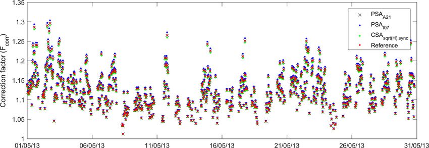
Figure 3. Flow chart of the data processing for the cumulative flux calculation using T of dataset D2 . FPSAI07 , FPSAA21 , FCSA√ , and
H ,sync
FREF are the cumulative fluxes corrected by following Fratini et al. (2012), in which Fcorr is calculated by implementing the time constants
(for PSA: τPSAI07 and τPSAA21 ; for CSA: τCSA√ ; for reference: τLPF ) calculated in previous section.
H ,sync
Fcorr was estimated using the method proposed by Fratini τLPF . We present the differences between cumulative fluxes
et al. (2012)1 : as relative differences with respect to the reference (FREF )
fRmax
in per cent. In particular, as an example, the relative bias
CO(f )df for PSAI07 is calculated as 100(FPSAI07 − FREF )/FREF while
f =fmin for CSA√H ,sync as 100(FCSA√H ,sync − FREF )/FREF for sev-
Fcorr = , (11) eral attenuation and SNR conditions. The relevant results are
fRmax p
CO(f ) Hemp (f )df shown in Sect. 4.3.
f =fmin
where CO equals the current T cospectrum when the ab-
4 Results and discussion
solute sensible heat fluxes exceeded 15 W m−2 . For small
fluxes we used a site-specific cospectral model (see Ap-
4.1 Time constant estimation with PSA
pendix C) for CO instead of parameterization of Fcorr pro-
posed by Ibrom et al. (2007a). To make sure that the analysis In order to illustrate the important steps in the data analysis
was not affected by low data quality, we removed the fluxes in PSA (e.g. low-pass filtering, noise superimposition, and
with low friction velocity (u∗ < 0.2 m s−1 ), unrealistic sen- noise removal only for PSAI07 ), here we show how the shape
sible heat fluxes and non-stationary conditions (Foken and of power spectra changes on a logarithmic scale for a few
Wichura, 1996), eliminating 554 half-hourly data points out SNR values (5, 3.3, and 2.5) and low-pass filtering condi-
of 1440 (ca. 38 %). tions (Fig. 4). The low-pass filter time constants (τLPF ) of
The time constant (τ ) in Hemp is estimated by either PSA 0.1, 0.3, and 0.5 s result in fc values beyond which the sig-
(i.e. τPSAI07 and τPSAA21 ) or CSA (i.e. τCSA√H ,sync ), and this nals become attenuated of ca. 1.6, 0.5, and 0.3 Hz. As the
yielded cumulative fluxes FPSAI07 , FPSAA21 , and FCSA√H ,sync , time constant increases, fc decreases, causing stronger atten-
respectively. For simplicity, in the FRC only median values uation. Referring to the upper panel of Fig. 4, for constant
of time constants of PSA and CSA ensembles estimated were attenuation (τLPF = 0.1 s), if the SNR decreases, noise be-
used for each combination of SNR and attenuation. The ref- comes more visible and the line fit to the noise becomes more
erence fluxes (FREF ) were also estimated with Fcorr using consistent. Similarly, referring to the left panel of Fig. 4,
1 Here we preferred using the square root to describe the true for constant SNR (e.g. for SNR = 5), from top to bottom,
transfer function as it is a good approximation when maximization as attenuation increases, the slope of the fit increases, and
of the cross-covariance is used for the time-lag correction as shown therefore the goodness of fit increases (Table 1). As dis-
by Peltola et al. (2021). cussed in Sect. 2.2, white noise causes a slope of 1, and thus
https://doi.org/10.5194/amt-14-5089-2021 Atmos. Meas. Tech., 14, 5089–5106, 20215096 T. Aslan et al.: The choice of the spectral correction method
Figure 4. Effect of several low-pass filtering (τLPF = 0.1, 0.3, and 0.5 s) and SNR (5, 3.3, and 2.5) on spectra of sonic temperature (T ) of
70 half-hourly data records illustrated in logarithmic scale, where f is natural frequency, ST is spectral density, and σT 2 is the variance of
T . Shown are the spectra of raw measured sonic temperature (red lines) and of the artificially deteriorated (i.e. low-pass filtered and noise
superimposed) sonic temperature before (dark blue) and after (black) noise removal following Ibrom et al. (2007a) through the subtraction
of the linear fit (dashed blue lines) to the high-frequency end of the deteriorated spectra. The vertical lines mark the frequency range used
for fitting for noise removal. The lower thresholds of the frequency range are 3, 2.3, and 2 Hz for the attenuation levels of 0.1, 0.3, and 0.5 s,
respectively.
Table 1. Results of the noise removal procedure applied in the of noise increases, while for PSAA21 it is small and almost
power spectra approach following Ibrom et al. (2007a) (PSAI07 ): constant with only a slight increase.
the values indicate the slopes of the fitted line to the high-frequency For PSAI07 , the optimal frequency domains used for noise
end of the spectrum in Fig. 4, with the coefficient of determination fitting were detected as 3, 2.6, and 2.3 to 5 Hz for the dif-
(R 2 ) shown in the parenthesis as a function of τLPF and SNR. Note ferent attenuation levels of 0.1, 0.2, and 0.3 s, respectively.
that for accurate noise removal the slopes should equal 1.
For attenuation levels of 0.4 and 0.5 s, we used the frequency
range of 2 to 5 Hz.
SNR = 5 SNR = 3.3 SNR = 2.5
PSAI07 overestimates the time constants with improving
τLPF = 0.1 s 0.57 (0.93) 0.78 (0.98) 0.87 (0.99) accuracy from low-attenuation to high-attenuation conditions
τLPF = 0.3 s 0.91 (0.99) 0.96 (0.99) 0.97 (0.99) regardless of the SNR values. The overestimation is likely
τLPF = 0.5 s 0.96 (0.99) 0.98 (0.99) 0.99 (0.99) due to the noise removal procedure, which further attenu-
ates the high-frequency end of the spectra by removing the
part of the signal together with noise (i.e. the noise is fit-
ted with a slope < 1). In this approach, the accuracy of the
any discrepancies from 1 result in overestimated noise re- noise removal procedure can be improved by visual inspec-
moval. Based on Fig. 4 alone, it is evident that removing the tion and adjustment of the fitting range to provide slopes
noise from power spectra can be done with higher accuracy close to 1 and thus better fitting parameters. However, es-
when the high-frequency attenuation increases and/or SNR pecially for low-attenuation conditions (e.g. 0.1, 0.2 s), the
decreases. frequency range is not sufficient to detect the noise statis-
The results of the time constant estimation are shown in tically, meaning that the linear fitting method is not ideal
Fig. 5a and 5b for PSAI07 and PSAA21 , respectively. Re- for differentiating in the spectral power the noise contribu-
sults are presented as medians with 25th and 75th percentile tion from the real variations due to turbulence. In addition
ranges for the repeat simulations. It can be seen that for to the shortcoming of the linear fitting, the visual inspection
PSAI07 the interquartile range (IQR) expands as the amount
Atmos. Meas. Tech., 14, 5089–5106, 2021 https://doi.org/10.5194/amt-14-5089-2021T. Aslan et al.: The choice of the spectral correction method 5097
Figure 5. Time constants calculated using the power spectrum approach, comparing (a) PSAI07 and (b) PSAA21 in several low-pass filter-
ing conditions (τLPF = 0.1–0.5 s) as a function of signal-to-noise ratio (SNR) over the range 10–1.1, which corresponds to the amount of
noise (e.g. 10 %–90 %). The solid black curve represents the median, while the shaded area represents interquartile ranges. The dashed line
corresponds to the expected value (τLPF ), which was used for the artificial low-pass filtering.
of detecting the frequency ranges for both noise removal and edge of the nature of the noise, which should be determined
the H fitting constitutes another uncertainty source due to in advance and implemented in Eq. (6) by adjusting the last
its subjectivity. It requires expertise on the topic and is hard term that characterizes the noise. This said, in many EC stud-
to automate when using software used for flux calculations ies, the type of noise is attributed to white noise (e.g. Launi-
(e.g. EddyPro). Moreover, in some cases, the optimal visual ainen et al., 2005; Peltola et al., 2014; Rannik et al., 2015;
inspection might not be sufficient as the low-attenuation re- Gerdel et al., 2017; Wintjen et al., 2020)2 but brown noise
sults in our study suggest. In our case we could not further in other studies (Wintjen et al., 2020). A simple approach
improve the accuracy even though the exact attenuation and to characterize the type of noise is either by examining the
SNR level were known, which is not the case with real-world high-frequency end of spectra, which is similar to our study,
data. or through the Allan variance, e.g. Werle et al. (1993). Al-
PSAA21 successfully estimates the time constants regard- ternatively, we conducted a brief investigation into the type
less of the attenuation and SNR level. This is due to using of noise by comparing the power spectra of measurements
the whole frequency range for fitting without separating the with very low SNR and those of white and blue noise (see
superimposed attenuated signal and noise. The most impor- Appendix B). It should be noted, however, that there are situ-
tant advantage of the PSAA21 is that it does not require visual ations when noise is complex and difficult to predict a priori.
inspection.
We assumed that the noise contaminating the signal is
2 This also includes Ibrom et al. (2007a), who falsely interpreted
white noise, which may not always be the case in real-world
data. Thus, the accuracy of the PSAA21 depends on knowl- the (white) noise as blue. This conclusion, however, was misguided
by neglecting the fact that the power spectra were multiplied by f .
https://doi.org/10.5194/amt-14-5089-2021 Atmos. Meas. Tech., 14, 5089–5106, 20215098 T. Aslan et al.: The choice of the spectral correction method
4.3 Effect of time constant variations on cumulative
fluxes
Figures 8 and 9 illustrate how variation in the estimation
method of the time constant affected the cumulative fluxes in
comparison to reference fluxes (see Sect. 3.3) calculated us-
ing dataset D2 . Figure 10 shows the correction factors (Fcorr )
for the case with τ = 0.3 s and SNR of 2. The values vary be-
tween 1 and 1.3, indicating the frequency response correction
as high as 30 %.
PSAI07 -based fluxes showed a bias varying between 0.1 %
and 1.5 %, whereas PSAA21 showed almost no bias, reflect-
ing the more accurate time constant estimation previously
shown. Fluxes based on CSA√H ,sync were close to the ex-
pected value with the bias of ±0.4 % with negligible re-
sponse to the SNR level. These findings are consistent with
the observed biases in time constant estimation, meaning that
Figure 6. Normalized ensemble cospectra for the original and var- where the time constant and the low-pass filtering were over-
ious attenuated time series (i.e. τ =0.1, 0.3, and 0.5 s). White noise estimated (e.g. with the PSAI07 especially for τ = 0.1 s and
was added at a signal-to-noise ratio (SNR) of 1.1. The red line repre- CSA√H ,sync for τ = 0.1 and 0.5 s), the spectral correction
sents the unattenuated and noise-free cospectrum, while the dashed, factor and thus the fluxes were overestimated, too. In sum-
dotted-dashed, and dotted lines show the noise-contaminated and mary, the findings indicate that using the PSAA21 for the
low-pass filtered cospectra for the three attenuation levels. time constant estimation provides quite accurate FRC. On
the other hand, for the CSA method, CSA√H ,sync reasonably
approximates the time constants, hence FRC. These results
4.2 Time constant estimation with CSA are in agreement with the analysis presented in Peltola et al.
(2021), showing that CSA√H ,sync approximates the effect of
Figure 6 illustrates the time-lag-corrected cospectra of three
phase shift on the estimation of the time constant and flux
low-pass filtered cases (i.e. τ = 0.1, 0.3, and 0.5 s) with the
correction factor. See Peltola et al. (2021) for more details.
most noisy conditions (i.e. lowest SNR of 1.1) in addition
to the unattenuated and noise-free cospectra (i.e. original). It
shows that the white noise contamination did not cause lin- 4.4 Review of typical signal-to-noise ratios and
ear increase in the high-frequency end of the cospectra, en- response times encountered during closed-path flux
abling the time-constant calculation without additional pro- measurements
cedure related to noise removal.
The range of attenuation and SNR conditions reported in
CSA√H ,sync successfully estimates the time constants
the literature is rather wide and varies depending on ecosys-
(Fig. 7). The variation around the expected values can be at-
tem type, the scalar of interest, data processing, a configu-
tributed to the shortcomings in the maximization of the cross-
ration of instruments, and set-up of the EC system. Ibrom
covariance used for the time-lag correction, the precision of
et al. (2007a) examined fluxes of water vapour and CO2 mea-
which is limited to the sampling interval (e.g. 0.1 s). Hence,
sured over a temperate forest, both of which were disturbed
the importance of the precision of time-lag detection can be
by noise in the high-frequency range of power spectra (see
noted as a shortcoming of CSA. The use of square root might
their Fig. 2). They identified an fc of CO2 as low as 0.325 Hz
be the another reason for the variation as it is an approxi-
(i.e. ca. τ = 0.5 s), indicating strong attenuation, while H2 O
mation, not an exact representation of the phase shift effect
showed even stronger attenuation which increased with rel-
(Peltola et al., 2021).
ative humidity to up to 0.010 Hz (i.e. ca. τ = 16 s) due to
Lastly, as expected, the level of noise does not affect the
the sorption/desorption effects on the sampling line internal
accuracy of the CSA method at any SNR level as the random
walls. Langford et al. (2015) reviewed SNR values of vari-
noise does not correlate with w, which is a pivotal advantage
ous gases published in many studies. In their comprehensive
of the CSA in general. It does, however, add random noise
analysis (their Fig. 4), the majority of the half-hourly datasets
to the result that is greater than in the improved PSAA21 ap-
of isoprene and acetone, measured with a quadrupole-based
proach.
proton transfer reaction-mass spectrometer (PTR-MS, Ion-
icon Analytik GmbH, Austria) above broad-leaf woodland,
roughly showed SNRs of 0.5 and 0.3, respectively, and ben-
zene measured (with the same instrument) in the urban en-
vironment showed an SNR of 0.3. Additionally, N2 O mea-
Atmos. Meas. Tech., 14, 5089–5106, 2021 https://doi.org/10.5194/amt-14-5089-2021T. Aslan et al.: The choice of the spectral correction method 5099
Figure 7. Time constants calculated using the cospectral approach, i.e. CSA√H ,sync , for several low-pass filtering conditions (τLPF = 0.1–
0.5 s) as a function of signal-to-noise ratio (SNR) over the range 10–1.1, which corresponds to the amount of noise (e.g. 10 %–90 %). The
solid black line represents the medians, while the shaded areas represent interquartile ranges. The dashed line corresponds to the expected
value (τLPF ), which was used for the artificial low-pass filtering.
Figure 8. Relative biases of the cumulative fluxes derived with Figure 9. Relative biases of the cumulative fluxes derived with the
different PSA methods, i.e. PSAI07 (blue) and PSAA21 (black), CSA√H ,sync compared with the reference flux as a function of SNR
compared with the reference flux as a function of SNR for differ-
for different attenuation timescales (0.1–0.5 s), calculated as, for ex-
ent attenuation timescales (0.1–0.5 s), calculated as, for example,
ample, 100(FCSA√ − FREF )/FREF .
100(FPSAI07 − FREF )/FREF . H ,sync
https://doi.org/10.5194/amt-14-5089-2021 Atmos. Meas. Tech., 14, 5089–5106, 20215100 T. Aslan et al.: The choice of the spectral correction method
Figure 10. Correction factors (Fcorr ) of half-hourly fluxes calculated with different approaches, i.e. PSAA21 (black cross), PSAI07 (blue
point), CSA√H ,sync (green point), and the reference (red point) for the case with τ = 0.3 s and SNR of 2.
sured with an older tunable diode laser (Aerodyne Research respect to SNR level and attenuation conditions. This pro-
Inc., Billerica, MA, USA) over managed grassland showed vides the opportunity to extend the results of this study be-
an SNR of 1. Rannik et al. (2016) examined the random un- yond the examined values and guides the selection of the
certainties in fluxes measured over forest, lake, and peatland right method to find the relevant H .
ecosystems in the boreal region. According to their unpub- The key constraint of the study was that we artificially
lished calculations, the SNRs of CO2 and H2 O measured simulated the various attenuation and SNR conditions. Thus,
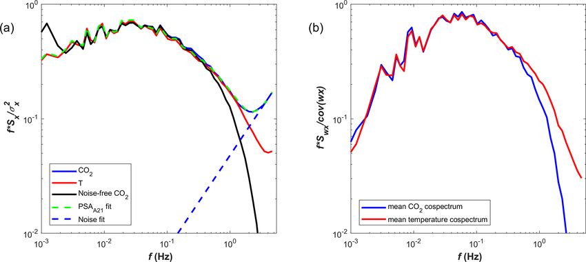
with an infrared gas analyser (LI-6262, LI-COR, Lincoln, demonstrating the performance of the methods with real-
NE, USA) were 2.6 and 10.3 for the forest site, respectively, world data is of great importance. Accordingly, here we pro-
while the SNRs of CO2 , H2 O, and CH4 measured with two vide an example via processing CO2 data D3 with the SNR
closed-path analysers (i.e. LI-7000, LI-COR, Lincoln, NE, of 2.3. The power spectra and cospectra of CO2 and T are
USA, for CO2 , H2 O, and FMA, and Los Gatos Research, Los shown in Fig. 11. The estimated time constants were 0.095,
Gatos, CA, USA for CH4 ) were 2.7, 24.3, and 5.4, respec- 0.075, and 0.173 s for PSAI07 , PSAA21 , and CSA√H ,sync , re-
tively. At the same forest site, Kohonen et al. (2020) investi- spectively. The details and statistics of fitting procedures are
gated fluxes of carbonyl sulfide (COS) with a newer genera- summarized in Table 2. The PSAA21 fit successfully approx-
tion Aerodyne quantum cascade laser spectrometer (QCLS) imates the noisy CO2 power spectra (R 2 = 0.993), enabling
(Aerodyne Research Inc., Billerica, MS, USA) that also mea- us to assume that the noise is white. However, the slope of
sures mole fractions of CO2 and H2 O. They reported high the linear noise fit of PSAI07 differs from 1 (0.82). We be-
attenuation for their measurement set-up (time constant of lieve that this is due to the low attenuation so that the noise
0.68 s for their EC system) and high noise disturbance in their cannot become visible similarly as in the case of the artifi-
power spectra (their Fig. 7) with an SNR of about 1. During cial dataset with low attenuation shown in Fig. 4, resulting
the measurement period, COS showed small fluxes near the in overestimation as it erroneously removes part of the signal
detection limit, causing uncertainty in the calculation of H . together with noise. The differences in time constants ob-
Thus, they calculated the time constant using the cospectra tained via PSA and CSA approaches might be attributed to
of CO2 , assuming that both fluxes are affected by the same sensor separation, uncertainties in time-lag correction, and
attenuation. the use of square root in CSA.
In addition, N2 O fluxes measured over urban areas (Järvi
et al., 2014) and CO2 fluxes over lake ecosystems (Mam-
marella et al., 2015) can also be examples of low SNR con- 5 Conclusions
ditions.
Given the wide range of SNR and attenuation conditions Here we investigated the limitations of two commonly used
summarized above, we analysed only a limited range of SNR approaches to empirically estimate the eddy-covariance (EC)
and attenuation. Also, the impact of the system response time transfer function needed for the frequency response correc-
depends on the position of the spectral peak frequency which tion of measured fluxes by analysing a temperature flux time
changes not only with wind speed but also measurement series which was synthetically degenerated mimicking slow-
height and surface roughness. Nevertheless, the analysis of response set-ups and noisy sensors. The first approach (PSA)
the different approaches showed a systematic behaviour with is based on the ratio of measured power spectra, while the
second (CSA) is based on the ratio of measured cospec-
Atmos. Meas. Tech., 14, 5089–5106, 2021 https://doi.org/10.5194/amt-14-5089-2021T. Aslan et al.: The choice of the spectral correction method 5101
Figure 11. (a) Power spectra of (1) sonic temperature (red), (2) CO2 from the Siikaneva site measured simultaneously with D1 (black), and
(3) noise-removed CO2 (dashed blue); shaded areas show the frequency range used for noise fitting for PSAI07 , and time constant fitting for
PSAI07 and PSAA21 . (b) Cospectra of CO2 (black) and T (red) with vertical wind speed (w).
Table 2. Time constants obtained via different approaches (PSAI07 , PSAA21 , and CSA√H ,sync ) for CO2 data from the Siikaneva site and
relevant statistics.
Method PSAI07 PSAA21 CSA√H ,sync
τ (s) 0.095 0.075 0.173
Coefficient of determination (R 2 ) of time constant fitting 0.989 0.993 0.958
Coefficient of determination (R 2 ) of noise fitting 0.99 – –
Slope of noise fitting 0.82 – –
Frequency range of noise fitting (Hz) 3.5–5 – –
Frequency range of time constant fitting (Hz) 0.01–2 0.01–5 0.01–2
Normalization factor (Fn ) 1.017 1.022 –
tra. For PSA, we examined two alternative approaches of random uncertainty in the case of noisy data. However, the
accounting for the white noise contribution to the power approach assumed that the signal is contaminated by white
spectra: i.e. PSAI07 and PSAA21 . The latter is newly in- noise, but this is not necessarily always the case. Hence, prior
troduced here and does not require noise removal prior to to the calculation of the time constant with this method, the
the fitting of the response function. For CSA, we examined nature of noise must be known. CSA√H ,sync showed a slight
one approach utilizing the square root of the transfer func- deviation from expected values. That can be attributed to lack
tion (H ) with shifted w time series via maximization of the of precision in time-lag estimation and the use of square root.
cross-covariance, i.e. CSA√H ,sync . We generated an artificial We then examined the effect of the different approaches to
dataset using T with differing degrees of low-pass filtering estimate the time constants on the cumulative fluxes: fluxes
(simulated damping) and additional random noise. The ad- corrected using the PSAI07 -based time constants showed the
vantage of using artificial datasets is that the real values of bias varying between 0.1 % and 1.5 % in comparison with
frequency attenuation, SNR, and physical time lag are all reference fluxes (see Sect. 3.3), for which PSAA21 showed al-
known, allowing the precise comparison of the estimations most no bias. By contrast, fluxes corrected using CSA√H ,sync
and expected values. PSAI07 overestimated the noise contri- showed the bias of ±0.4 %. This analysis, however, does not
bution and consequently the signal loss and time constant account for the shortcomings of the method, i.e. Fratini et al.
for low-attenuation conditions, but better performance was (2012), and thus should be read as the sole effect of time
found as attenuation increases. The new PSAA21 approach constant estimation on the final fluxes. The comparison of
successfully estimated the time constants regardless of the commonly used methods are comprehensively done in the
attenuation and SNR level, identifying the noise and sig- companion paper.
nal comprehensively and providing no bias and the lowest
https://doi.org/10.5194/amt-14-5089-2021 Atmos. Meas. Tech., 14, 5089–5106, 20215102 T. Aslan et al.: The choice of the spectral correction method The SNR did not affect the accuracy of either PSA or CSA Finally, given the constraints of this study, we encourage approaches, alleviating concerns on EC flux measurements additional studies based on the real attenuation and SNR con- with low SNR levels. ditions, investigating also other types of noise contamination In summary, for the empirical estimation of parameters to provide a step forward in efforts to standardize the EC of H of closed-path EC systems, our findings showed that method, which is of great importance to avoid systematic bi- PSAA21 is the most accurate, precise, and robust method ases of fluxes and improve comparability between different when power spectra are used. This finding was independent datasets. of SNR and degree of attenuation. On the other hand, using the square root of H in CSA√H ,sync , which is a good ap- proximation of the attenuation of cospectra in the presence of phase shifts (Peltola et al., 2021), provided the reasonably correct estimation of τ and Fcorr when cospectra are com- puted after with time-lag quantification by cross-covariance maximization. Atmos. Meas. Tech., 14, 5089–5106, 2021 https://doi.org/10.5194/amt-14-5089-2021
T. Aslan et al.: The choice of the spectral correction method                                                                             5103

Appendix A: Derivation of the PSAA21

In this section, we derive the new approach for the PSA
(i.e. PSAA21 ) in detail. We assume that the measured χ con-
tains two independent and additive components: the atten-
uated turbulent signal and the noise. We further assume that
scalar similarity holds (i.e. power spectra of all scalars follow
a similar shape). After these assumptions the power spectrum
(Sχ ) of χ can be written as

               σχ2
Sχ (f ) =            H ST (f ) + Sχ,n (f ),                        (A1)
               σT2

where σχ2 and σT2 are the variances of χ and T related to tur-
bulent signal (no attenuation or noise), ST (f ) is the power
spectrum of T , H describes the attenuation of χ due to
imperfect instrumentation, and Sχ,n is the noise in the χ                  Figure B1. Normalized spectra of methane concentration (red),
measurements. Note that here the noise in the T measure-                   white noise (black), and blue noise (blue) (f Ss /σs2 ), all of which
                                                                           have the same standard deviation. The solid straight line is f +1
ments was neglected as being small except in very low turbu-
                                                                           line.
lence conditions (when eddy-covariance measurements be-
come problematic anyway and fluxes are removed by the u∗
filter). Assuming that the instrument measuring χ can be
approximated by a first-order linear sensor and reordering
terms, this yields                                                         Appendix B: Identification of instrumental noise

Sχ (f ) ST (f )          1         Sχ,n (f )
       =        Fn               +           ,                     (A2)    Here we perform a short analysis to characterize the type of
 σχ2     σT 2      1 + (2πf τ )2     σχ2                                   noise in an example high-frequency CH4 time series by com-
where the proportionality constant Fn was introduced due to                paring the spectra of a turbulent scalar with those of artifi-
the effect that noise adds to σχ2 and thus biases the normal-              cially generated white and blue noise.
ization (see Ibrom et al., 2007a). The spectral density is best               Methane fluxes from an upland forest site can be con-
shown in log–log space as a wide range of frequencies, and                 sidered to be greatly affected by instrumental noise because
spectral densities are well displayed (Stull, 2012), with nat-             fluxes are small and near the detection limit. Therefore, we
ural frequency (f ) on the x axis and spectral density multi-              used a forest methane mixing ratio dataset to identify the type
plied by f on the y axis. After multiplication by f , Eq. (A2)             of noise by comparing its spectra with the spectra of white
becomes                                                                    and blue noise which was artificially generated and with the
                                                                           same standard deviation of the methane dataset.
    Sχ (f )    ST (f )          1           Sχ,n (f )                         The data were collected at the SMEAR II station (Station
f           =f         Fn                +f           .            (A3)
     σχ2        σT 2      1 + (2πf τ ) 2      σχ2                          for Measuring Forest Ecosystem–Atmosphere Relations),
                                                                           Hyytiälä, southern Finland (61◦ 510 N, 24◦ 170 E; 181 m a.s.l.),
                                         Sχ,n (f )
    As described in Sect. 2.2, f                     can be approximated   which is a class 1 Integrated Carbon Observation Sys-
                                           σχ2
by a model that is linear in frequency in logarithmic space                tem (ICOS) ecosystem station. The station is surrounded
     S (f )                                                                by extended areas of coniferous forests, and the EC tower
as f χ,n
      σ2
            = a log(f ) + log(b). In the case of white noise,
           χ                                                               is located in a 55-year-old (in 2017) Scots pine (Pinus
where a = 1, this results in a simplified linear model as                  sylvestris L.) forest with a dominant tree height of 19 m.
 S (f )
f χ,n
   σ2
        = log(f ) + log(b) and in non-logarithmic space as                 The measurements were performed with 10 Hz sampling fre-
       χ
                                                                           quency at a height of 23 m, i.e. approximately 4 m above the
elog(f )+log(b) , which is f b. Substitution into Eq. (A3) yields
                                                                           forest canopy. A fast response laser absorption spectrometer
    Sχ (f )    ST (f )          1                                          (G2311-f, Picarro, Santa Clara, CA, USA) was used to mea-
f       2
            =f     2
                       Fn               + f b.                     (A4)    sure the CH4 mixing ratio.
     σχ         σT        1 + (2πf τ )2
                                                                              Power spectra of methane were calculated using mea-
   It is worth mentioning that this method can be used to                  surements from 10 July at 12:00–14:30 UTC+2. The high-
retrieve the variance of noise as well since b equals the                  frequency range of the normalized frequency-weighted CH4
ensemble-averaged noise power spectra (Sχ,n ) divided by                   power spectrum follows the f +1 power law scaling, which is
σχ2 . However, we do not further examine it as it is not the               consistent with white noise and inconsistent with, for exam-
main interest of this study.                                               ple, blue noise (Fig. B1).

https://doi.org/10.5194/amt-14-5089-2021                                                      Atmos. Meas. Tech., 14, 5089–5106, 2021
You can also read