Evolutionary Image Transition and Painting Using Random Walks
←
→
Page content transcription
If your browser does not render page correctly, please read the page content below
Evolutionary Image Transition and Painting
                                                        Using Random Walks

                                        Aneta Neumann                                      aneta.neumann@adelaide.edu.au
                                        Optimisation and Logistics, School of Computer Science, The University of Adelaide,
arXiv:2003.01517v1 [cs.NE] 2 Mar 2020

                                        Australia
                                        Bradley Alexander                                bradley.alexander@adelaide.edu.au
                                        Optimisation and Logistics, School of Computer Science, The University of Adelaide,
                                        Australia
                                        Frank Neumann                                      frank.neumann@adelaide.edu.au
                                        Optimisation and Logistics, School of Computer Science, The University of Adelaide,
                                        Australia

                                        Abstract
                                            We present a study demonstrating how random walk algorithms can be used for evo-
                                            lutionary image transition. We design different mutation operators based on uniform
                                            and biased random walks and study how their combination with a baseline mutation
                                            operator can lead to interesting image transition processes in terms of visual effects and
                                            artistic features. Using feature-based analysis we investigate the evolutionary image
                                            transition behaviour with respect to different features and evaluate the images con-
                                            structed during the image transition process. Afterwards, we investigate how modi-
                                            fications of our biased random walk approaches can be used for evolutionary image
                                            painting. We introduce an evolutionary image painting approach whose underlying
                                            biased random walk can be controlled by a parameter influencing the bias of the ran-
                                            dom walk and thereby creating different artistic painting effects.

                                        1     Introduction
                                        Evolutionary algorithms (EAs) have been widely and successfully applied in the ar-
                                        eas of art (Antunes et al., 2015; Hingston et al., 2008; Lambert et al., 2013; McCormack
                                        and d’Inverno, 2012b; Neumann and Neumann, 2018a, 2019; Romero and Machado,
                                        2008). In this application area, the primary aim is to evolve artistic and creative outputs
                                        through an evolutionary process (al-Rifaie and Bishop, 2013; Greenfield, 2015; McCor-
                                        mack and d’Inverno, 2012a; Neumann and Neumann, 2018b; Neumann et al., 2017b;
                                        Vinhas et al., 2016). The use of evolutionary algorithms for the generation of art has
                                        attracted strong research interest. Different representations have been used to create
                                        works of greater complexity in 2D and 3D (Greenfield and Machado, 2015; Machado
                                        and Correia, 2014; Todd and Latham, 1992), and in image animation (Hart, 2007; Neu-
                                        mann et al., 2019b; Sims, 1991; Trist et al., 2011). The great majority of this work relates
                                        to the use of evolution to produce a final artistic product in the form of a picture, sculp-
                                        ture, animation.
                                        1.1    Related work
                                        In the seminal work the Blind Watchmaker, Dawkins (1986) investigated the process of
                                        evolution. He evolved figures called biomorphs in order to explore and to visualize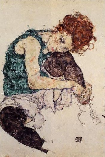
the power of evolution. The biomorphs’ appearance changes/diverges broadly from
the original parent over time demonstrating a simple model of bio-inspired evolution.
Inspired by Dawkins’ work, Sims (1991) created complex and imaginative images. He
used an expression-based approach to evolve images using a mathematical expression
as the genotype and applied crossover and mutation. In the interactive media installa-
tion Galapagos, visitors were able to evolve virtual creatures based on Darwinian evo-
lution principles whilst taking into account their own preferences (Sims, 1997). The
abstract organisms were displayed on computer screens and users interactively chose
virtual organisms for simulated growth by stepping onto selected pads. This exhibi-
tion was a visualization example of a collaboration process between the visitors and
the machine.
      Latham (1985) created a black and white lithographic artwork called Black Form
Synth consisting of hand-drawn ”evolutionary trees of complex forms” in the form of
a flow diagram arranged with a set of transformation rules. Following the expression-
based approach, Latham (1989) extended the rule-based evolutionary approach in or-
der to invent new complex 3D forms from geometric primitives. Todd and Latham
(1992) introduced the framework called Mutator to generate art and evolve new 3D
biomorphic forms. The Mutator creates a series of complex branching organic forms
and surreal virtual sculptures, and animated videos through the process of ”surreal”
evolution. At each iteration the artist selects phenotypes based on the idea of evolved
organisms that are able to “breed and grow”.
      Over time, the growing interest in an expression-based approach led to expan-
sion of the area of evolutionary art, providing coherent and solid basis for further
research (Fenton et al., 2017a; Paauw and van den Berg, 2019; Richter, 2018; Urbano,
2018). Hart (2007) used an expression-based approach with the focus of evolving a set
of images with a different appearance to the previous works. This system’s interface
allowed a greater range of control over the colors and forms of the evolved images.
Complex and detailed images were created in Rooke (2006) using an expression-based
approach guided by aesthetic selection, in particular towards the evolution of color
space. Unemi (2004, 2012) continued to explore the expression-based approach to
evolutionary art by evolving images and animations towards the progression of color
volumes and novel forms with varied variables. The images are evolved based on aes-
thetic measures and have been displayed on the internet for decades using different
versions of the SBART framework (Unemi, 1999). Machado and Cardoso (2002) intro-
duced computer-aided software, called NEvAr. This is an evolutionary art tool which
uses: genetic programming, user-guided evolution, and automatic fitness assignment.
The model uses a fitness function that permits aesthetically pleasing and visually com-
plex images. Draves (2005) introduced Electric Sheep, a large and ongoing evolution-
ary art project using collective human evaluation. It was implemented as a distributed
screen-saver allowing users to approve or disapprove phenotypes in order to evolve ar-
tificial life and is focused on the continuing behavior of the distributed system. Green-
field (2006) describes simulated robots embedded into an evolutionary framework for
the purpose of painting a new artwork. The system implements optimization towards
identifying robot paintings with higher aesthetic properties and takes into account the
behavior of the simulated robots.
      Aesthetic feature measures have been widely applied to generate new artistic im-
ages (Heaton, 2019; Lewis, 2008; Neumann et al., 2018b). The evolutionary art system
NEvAr, Machado and Cardoso (2002) used aesthetic measures and evolutionary com-
putation methods, and thus developed automatic seeding procedures to generate im-

                                           2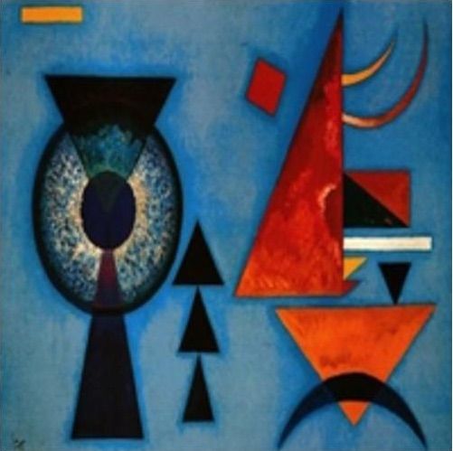
ages. Greenfield (2002) evolved images using computational aesthetic functions that
are based on a color segmentation algorithm. Moreover, den Heijer and Eiben (2014)
studied aesthetic measures in unsupervised evolutionary art using aesthetic measures
as fitness functions.
      In Interactive Evolutionary Computation (IEC), the traditional objective-function is
replaced by a human subject who guides the selection (Takagi, 2001). In IEC, each so-
lution is evaluated by a human judgment. Those subjective choice provides the basis
for the selection of solutions in the evolutionary process. IEC founds its biggest ap-
plication in the creative domains in which including humans ‘in the loop can lead to
novel solutions (Fenton et al., 2017b; Hingston et al., 2008; Hollingsworth and Schrum,
2019; Romero and Machado, 2008; Takagi, 2001). In this case, the fitness function is
based on the individual user’s experiences and preferences towards interesting or aes-
thetic results. This means that the fitness of the evolutionary algorithm (EA) is strongly
subjective.
      In contrast to this, a different approaches evaluate artistic images by automate fit-
ness evaluation in order to generate novel images. Baluja et al. (1994) attempted to
automate the process of image evolution by using neural networks in order to produce
images. The primary idea was to learn the user’s preferences, and to apply this insight
to generate aesthetically pleasing images. Moreover, den Heijer and Eiben (2014) pre-
sented an approach for evolving images without human interaction. Instead of human
interaction, they used one or more aesthetic measures as fitness functions to guide the
search. They investigated the correlation between aesthetic scores in order to calculate
which aesthetic measure generate images that are evaluated positively by the other
aesthetic measures.
      Another application of evolutionary algorithms to art is the creation of image tran-
sitions. Graf and Banzhaf (1995) used interactive evolution to help determine param-
eters for image morphing. They combined interactive evolutionary computation with
the concept of warping and morphing from computer graphics to evolve images. More
precisely, they used the recombination of two bitmap images through image interpola-
tion. Furthermore, Karungaru et al. (2007) used an evolutionary algorithm to automat-
ically identify features for morphing faces.
      More recently, deep neural networks have been used to create artistic images
through the transfer of artistic style from one image to another, facilitating novel forms
of image manipulation (Gatys et al., 2016b). A new neural style transfer approach pre-
serves the colors of the original image using simple linear methods for transferring
style. Gatys et al. (2016a, 2017) extended the existing method by introducing control
over colour information, spatial scale, and spatial location. Johnson et al. (2016) com-
bined the benefits of both approaches, trained feed-forward convolutional neural net-
works and perceptual loss functions based on high-level features extracted from pre-
trained networks and proposed the use of perceptual loss functions for training feed-
forward networks for image transformation. The transfer of style from one image to
stable video sequences was proposed by new initializations and loss functions applica-
ble to videos in Ruder et al. (2016).
      Furthermore, inspired by the work of Gao et al. (2016), evolutionary diversity op-
timization have been applied to evolve images in one/two aesthetic feature dimen-
sions (Alexander et al., 2019, 2017; Neumann et al., 2018a). Building on these studies,
Neumann et al. (2019a) introduced evolutionary diversity optimization for images us-
ing popular indicators from the area of evolutionary multi-objective optimisation.
      Non-photorealistic rendering (NPR) is an area of computer graphics that fo-

                                            3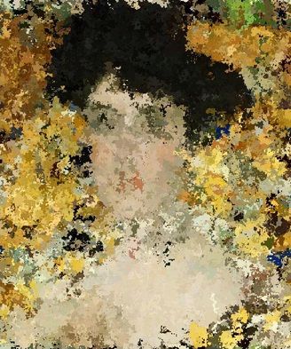
cuses on enabling a wide variety of expressive styles for digital art (Strothotte and
Schlechtweg, 2002). In contrast to traditional computer graphics, which has focused
on photorealism, NPR is inspired by artistic styles such as painting, drawing, technical
illustration, and animated cartoons. Litwinowicz (1997) described transformations
from ordinary video segments into animations that appear similar to hand-painted
techniques. In particular, they used modified off-the-shelf image processing and ren-
dering techniques in order to process images and videos for an impressionist effect.
Kubelka (1948) introduced the optical properties model in order to simulate the optical
effect of different layers of artwork. Hertzmann (1998) generated hand-painted images
by using series of different brush stroke sizes and orientations to generate images.
     In recent years, several evolutionary approaches for the production of non-
photorealistic renderings of images have been introduced (Barile et al., 2008; Izadi et al.,
2010; Kang et al., 2005; Machado and Pereira, 2012; Tao Wu, 2018).
     Furthermore, extensive research has been carried out on swarm painting. Urbano
(2006) investigated choices inside a group of agents in order to design swarm art
with interesting random patterns. Monmarché et al. (1999) used the stochastic and ex-
ploratory principles of an ant colony to automatically discover clusters in data without
prior knowledge of the structure of the data.
     A swarm-based system was used as a method to create visualizations of data,
and in order to combine information aesthetics with data visualization (Maçãs et al.,
2015). Boyd et al. (2004) created a collaborative project called Swarm Art that incor-
porated the swarm-based simulation and projected the artwork onto a large screen.
Greenfield (2005) used a colony optimization model to evolve ant paintings and inves-
tigated the effects of different fitness measures on the generation of different artistic
styles. Inspired by natural phenomena, namely the use of pheromone substances for
mass recruitment in ants’ pattern behaviour, Urbano (2005) generated collective artistic
work by embedding a pheromone medium pattern into the painters’ behaviour.

1.2   Our Contribution
 Neumann et al. (2016) described an image transition process where the key idea is to
use the evolutionary process itself in an artistic way. The focus of our paper is to study
how random walk algorithms can be used in the evolutionary image transition process
defined in Neumann et al. (2016) as mutation operators. We consider the well-studied
(1+1) EA, popular random walk algorithms and provide a new approach to evolution-
ary art by using theoretical approaches for evolutionary image transition. The transi-
tion process consists of evolving a given starting image S into a given target image T
by random decisions. Considering an error function which assigns to a given current
image X the number of pixels where it agrees with T and maximizes this function boils
down to the classical O NE M AX problem for which numerous theoretical results on the
runtime behaviour of evolutionary algorithms are available (Jansen and Sudholt, 2010;
Sudholt, 2013; Witt, 2013). An important topic related to the theory of evolutionary
algorithms are random walks (Dembo et al., 2004; Lovász, 1996). We consider random
walks on images where each time the walk visits a pixel its value is set to the value of
the given target image. By biasing the random walk towards pixels that are similar to
the current pixel we can study the effect of such biases which might be more interest-
ing from an artistic perspective. After observing these two basic random processes for
image transition, we study how they can be combined to give the evolutionary process
interesting new properties. We study the effect of running random walks for short pe-
riods of time as part of a mutation operator in a (1+1) EA. Furthermore, we consider

                                             4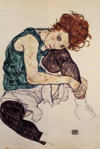
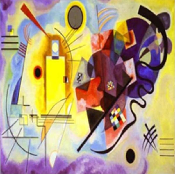
Figure 1: Starting image X (Yellow-Red-Blue, 1925 by Wassily Kandinsky) and target
image T (Soft Hard, 1927 by Wassily Kandinsky).

the effect of combining them with the asymmetric mutation operator for evolution-
ary image transition introduced in Neumann et al. (2016). Our results show that the
area of evolutionary image transition based on random walks provides a rich source of
artistic possibilities for creating video art. All our approaches are pixel-based and cre-
ated videos based on the evolutionary processes show frames corresponding to images
that were created every few hundred generations. After introducing these different ap-
proaches to evolutionary image transition based on random walks, we study their be-
haviour with respect to different aesthetic features. Feature-based analysis of heuristic
search methods has gained increasing interest in recent years (Mersmann et al., 2013,
2010; Nallaperuma et al., 2013). In other application areas feature-based analysis is
an important method to increase the theoretical understanding algorithm performance
and particularly useful for algorithm selection and configuration (Nallaperuma et al.,
2015; Neumann and Poursoltan, 2016). For evolutionary image transition, we study
how artistic features behave during the transition process. This allows the measure-
ment of the evolutionary image transition process in a quantitative way and provides
a basis to compare our different approaches with respect to artistic measures 1 .
      This article extends its conference version (Neumann et al., 2017a) in several ways.
Firstly, by investigations on the impact of random walk lengths for image transition in
Section 4.2 and the impact of the bias of the random walks controlled by the parameter
α in Section 4.3. Large values of α increase the probability of moving to similar color
pixel and different values of α lead to different image transition processes. Secondly,
we investigate how random walk algorithms can be used to carry out painting of im-
ages in Section 7. The key idea is to use a biased random walk starting at a given pixel
and color all pixels visited by the walk with the color of the starting pixel. We use the
biased random walk mutation approach introduced for evolutionary image transition
and combine it with the asymmetric mutation operator. Our approach starts a biased
random walk for each pixel to be changed by asymmetric mutation. To achieve differ-
ent effects of evolutionary image painting, we consider the parameter α which allows
to control of the bias of the random walk towards similar color pixels. Our experimen-
tal results show the effect of the setting of α for images of various types.
      The outline of the paper is as follows. In Section 2, we introduce the evolution-
ary transition process. In Section 3, we study how variants of random walks can be
used for the image transition process. We examine the use of random walks as part
  1 Images   and videos are available at https://vimeo.com/anetaneumann

                                                5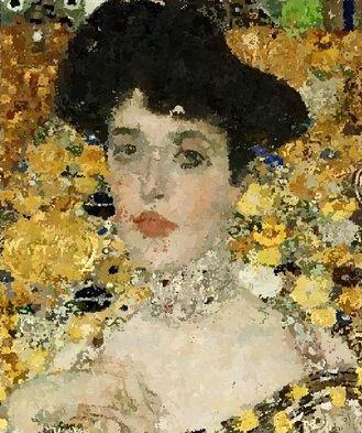
Algorithm 1 (1+1) EA for evolutionary image transition

    • Let S be the starting image and T be the target image.
    • Set X:=S.
    • Evaluate f (X, T ).

    • while (not termination condition)
        – Obtain image Y from X by mutation.
        – Evaluate f (Y, T )
        – If f (Y, T ) ≥ f (X, T ), set X := Y .

of mutation operators and study their combinations with asymmetric mutation during
the evolutionary process in Section 4. Furthermore, we extend our investigation on
the impact of different random walk length in biased random walk mutation and on
the impact of the chosen α in biased random walk mutation. In Section 5, we analyse
the different approaches for evolutionary image transition with respect to aesthetic fea-
tures. Our evolutionary painting algorithm using biased random walks is introduced
and evaluated in Section 6. Finally, we finish with some conclusions and future work.

2    Evolutionary Image Transition
We consider the evolutionary image transition process introduced in Neumann et al.
(2016). It transforms a given image S = (Sij ) of size m × n into a given target image
T = (Tij ) of size m × n. This is done by producing images X for which Xij ∈ {Sij , Tij }
holds. Given a starting image S = (Sij ) a target image T = (Tij ), and a current image
X = (Xij ), we say that pixel Xij is in state s if Xij = Sij , and Xij is in state t if
Xij = Tij . Our goal is to study different ways of using random walk algorithms for
evolutionary image transition.
      Throughout this paper, we assume that Sij 6= Tij as pixels with Sij = Tij can not
change values and therefore do not have to be considered in the evolutionary process.
To illustrate the effect of the different methods presented in this paper, we consider the
work Yellow-Red-Blue, 1925 by Wassily Kandinsky as the starting image and the work
T Soft Hard, 1927 by Wassily Kandinsky as the target image (see Figure 1). In principle,
this process can be carried out with any starting and target image. Using artistic im-
ages in this setting has the advantage that artistic properties of images are transformed
during the evolutionary image transition process. We will later on in this paper study
how the different operators used in the algorithms influence artistic appearance in re-
spect to different artistic features. At the beginning of the 20th century the well-known
artist Wassily Kandinsky was part of the famous Bauhaus movement (Droste, 2002).
Kandinsky was a unique university teacher in Weimar and Dessau and an iconic pro-
moter of a theory of geometric figures and their relationships. In the work ”Point and
Line to Plane”, Kandinsky and Rebay (1926) show an innovative approach to artistic
expression and to the creation of abstract paintings.
      We use the fitness function for evolutionary image transition used in Neumann
et al. (2016) and measure the fitness of an image X as the number of pixels where X and
T agree. This fitness function is equivalent to the O NE M AX problem when interpreting

                                                   6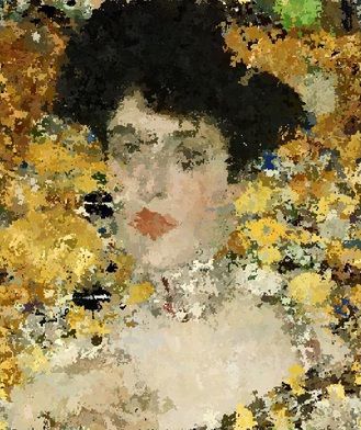
Algorithm 2 Asymmetric mutation

  • Obtain Y from X by flipping each pixel Xij of X independently of the others with
    probability cs /(2|X|S ) if Xij = Sij , and flip Xij with probability ct /(2|X|T ) if
    Xij = Tij , where cs ≥ 1 and ct ≥ 1 are constants, we consider m = n.

Figure 2: Image Transition using asymmetric mutation with cs = 100 and ct = 50 at
12.5%, 37.5%, 62.5% and 87.5% of the target image (from left to right).

the pixels of S as 0’s and the pixels of T as 1’s. Hence, the fitness of an image X with
respect to the target image T is given by

                           f (X, T ) = |{Xij ∈ X | Xij = Tij }|.

     We consider simple variants of the classical (1+1) EA in the context of image tran-
sition. The algorithm is using mutation only and accepts an offspring if it is at least
as good as its parent according to the fitness function. The approach is given in Al-
gorithm 1. Using this algorithm has the advantage that the parent and offspring only
differ by a small number of pixels which allows a smooth transition process. This en-
sures a smooth process for transitioning the starting image into the target. Furthermore,
we can interpret each step of the random walks flipping a visited pixel to the target out-
lined in Section 3 as a mutation step which, according to the fitness function, is always
accepted.
     As the baseline mutation operator, we consider the asymmetric mutation oper-
ator which has been studied in the area of runtime analysis for special linear func-
tions (Jansen and Sudholt, 2010) as well as the minimum spanning tree problems (Neu-
mann and Wegener, 2007). Using this mutation operator instead of standard bit mu-
tations for O NE M AX problems avoids the coupon collector’s effect (Kobza et al., 2007;
Mitzenmacher and Upfal, 2005). In the transition process, the coupon collector’s effect
implies that the last (even small) fraction of the pixels that need to be flipped to the
target need more time to be flipped than all the pixels previously set to the target. More
precisely, flipping each bit with probability 1/n as done in standard bit mutations, im-
plies that the waiting time to flip the last pixel to the target is Θ(n) whereas increasing
the number of target pixels is Θ(1) if the number of target pixels is still a constant frac-
tion of all the pixels. Such a slow-down at the end of the transition process where there
is no progress for many iterations is not desirable.
     We use the generalization of this asymmetric mutation operator already proposed
in Neumann et al. (2016) and shown in Algorithm 2. Let |X|T be the number of pixels
where X and T agree. Similarly, let |X|S be the number of pixels where X and S agree.
Each pixel in starting state s is flipped with probability cs /(2|X|S ) and each pixel in

                                             7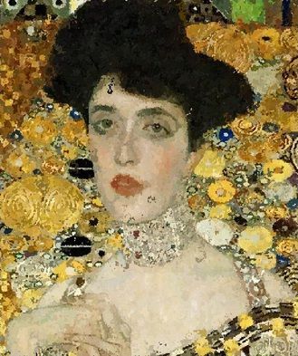
Algorithm 3 Uniform Random Walk

  • Choose the starting pixel Xij ∈ X uniformly at random.

  • Set Xij := Tij .
  • while (not termination condition)
       – Choose Xkl ∈ N (Xij ) uniformly at random.
       – Set i := k, j := l and Xij := Tij .

  • Return X.

target state t is flipped with probability ct /(2|X|T ). The special case of cs = ct = 1 has
been mathematically analyzed with respect to the runtime behaviour on other pseudo-
Boolean functions.
     We set the parameters as follows: cs = 100 and ct = 50. This allows both a decent
and sufficient speed for the image transition process and enough exchanges of pixels for
an interesting evolutionary process. We should mention that obtaining the last pixels of
the target image may take a long time compared to the other progress steps when using
large values of ct . However, for image transition, this only effects steps when there are
at most ct /2 source pixels remaining in the image. From a practical perspective, this
means that the evolutionary process has almost converged towards the target image
and setting the remaining missing target pixels to their target values provides an easy
solution.
     All experimental results for evolutionary image transition in this paper are shown
for the process of moving from the starting image to the target image given in Figure 1
where the images are of size 200 × 200 pixels. The algorithms have been implemented
in MATLAB. In order to visualize the process, we show the images obtained when the
evolutionary process reaches 12.5%, 37.5%, 62.5% and 87.5% pixels of target image for
the first time. We should mention that all processes except the use of the biased random
walks are independent of the starting and target image which implies that the use of
other starting and target images would show the same effects in respect to the way that
target pixels are displayed during the transition process.
     In Figure 2 we show the experimental results of the asymmetric mutation approach
as the baseline. On the first image from left we can see the starting image S with lightly
stippling dots in randomly chosen areas of the target image T . Consequently, the area
of the yellow dimensional abstract face disappears, and black and red abstract figure
appears. Meanwhile the background has adopted a dot pattern, where a nuance of dark
and light develops steadily. In the last image, we barely see the starting image S and the
target image T appearing permanently with the background becoming a darker blue
tone, whereby the stippling effect shown in the middle two frames decreases. Interest-
ing images in respect to aesthetic and evolutionary creativity emerge for the pictures
at 37.5% and 62.5% of the evolutionary processes. In the third picture, we can observe
elements of both images compounded with a very special effect as a result of the image
transition process.

                                               8
Algorithm 4 Biased Random Walk

    • Choose the starting pixel Xij ∈ X uniformly at random.

    • Set Xij := Tij .
    • while (not termination condition)
        – Choose Xkl ∈ N (Xij ) according to probabilities p(Xkl ).
        – Set i := k, j := l and Xij := Tij .

    • Return X.

Figure 3: Image Transition for Uniform Random Walk (top) and Biased Random Walk
(bottom) with 12.5%, 37.5%, 62.5% and 87.5% of the target image (from left to right).

3    Random Walks for Image Transition
Our evolutionary algorithms for image transition build on random walk algorithms
and use them later on as part of a mutation step. Specifically, we investigate the use of
random walk algorithms for image transition which move, at each step, from a current
pixel Xij to one of 4-connected pixels in its neighbourhood.
     We utilize the neighbourhood N (Xij ) of Xij following von Neumann’s definition
of neighbourhood (von Neumann, 1966) as

                         N (Xij ) = {X(i−1)j , X(i+1)j , Xi(j−1) Xi(j+1) }
where we work modulo the dimensions of the image in the case that the values leave
the pixel ranges, i ∈ {1, . . . , m}, j ∈ {1, . . . , n}. This implies that from a current pixel,
we can move up, down, left, or right. Furthermore, we wrap around when exceeding
the boundary of the image. We do this in order to have a more interesting process.
Furthermore, it supports the effectiveness of our biased random walks in the case that
they would be biased towards the image boundary. Not wrapping around in this case

                                                9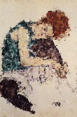
would imply that pixels opposite of the focused boundary can hardly be reached.
     The classical random walk shown in Algorithm 3 chooses an element Xkl ∈
N (Xij ) uniformly at random (Pearson, 1905). We call this the uniform random walk in
the following. The cover time of the uniform random walk on a n × n torus is upper
bounded by 4n2 (log n)2 /π (Dembo et al., 2004) which implies that the expected num-
ber of steps of the uniform random walk until the target image is obtained (assuming
m = n) is upper bounded by 4n2 (log n)2 /π)).

3.1   Biased Random Walk
We also consider a biased random walk where the probability of choosing the element
Xkl is dependent on the difference in RGB-values for Tij and Tkl . We favour a neighbor
Xkl ∈ N (Xij ) if Tkl is close to Tij in respect to RGB-values. The approach is shown in
Algorithm 4. Weighted random walks have been used in a similar way in the context
of image segmentation (Grady, 2006). We denote by Tijr , 1 ≤ r ≤ 3, the rth RGB value
of Tij and define
                                           ( 3                           )!α
                                            X
                                                    r
                        γ(Xkl ) =    max          |Tkl   −   Tijr |, 1         ,
                                            r=1

where α ≥ 0.
    In our random walk, we prefer Xkl if γ(Xkl ) is small compared to the other ele-
ments in N (Xij ). In order to compute the probability of moving to a new neighbour
we consider (1/γ(Xkl )) ∈ [0, 1] and prefer elements in N (Xij ) where this value is large.
    In the biased random walk, the probability of moving from Xij to an element Xkl ∈
N (Xij ) is given by

                                                (1/γ(Xkl ))
                          p(Xkl )   =   P                            .
                                           Xst ∈N (Xij ) (1/γ(Xst ))

      Our standard biased random walk works with α = 1 and we extend our investiga-
tions to other choices of α as part of our random walk mutation operator in Section 4.3.
Furthermore, we use different choices of α for image painting in Section 7. It should
be noted that the uniform random walk given in Algorithm 3 is the special case of
Algorithm 4 where α = 0.
      The biased random walk is dependent on the target image when carrying out mu-
tation or random walk steps and the importance of moving to a pixel with similar color.
By introducing the bias in respect to pixels that are similar, the bias can cause the evolu-
tionary image transition process to take exponentially long as the walk might encounter
effects similar to the gambler’s ruin process (Mitzenmacher and Upfal, 2005). For our
combined approaches described in the next section, we use the random walks as mu-
tation components which ensures that the evolutionary image transition is carried out
efficiently. We will use the biased random walk for evolutionary image transition in
Section 4.
      In Figure 3 we show the experimental results of the uniform random walk and
biased random walk. At the beginning, we can observe the image with the character-
istic random walk pathway appearing as a patch in the starting image S. Through the
transition process, the clearly recognisable patches on the target image T emerge. In
the advanced stages, the darker patches from the background of the target image dom-

                                             10
Figure 4: Image Transition for EA-UniformWalk (top) and EA-BiasedWalk (bottom)
with 12.5%, 37.5%, 62.5% and 87.5% of the target image (from left to right).
inate. The effect in animation is that the source image is scratched away in a random
fashion to reveal an underlying target image.
The four images of the biased random walk are clearly different to the images of the
uniform random walk. During the course of the transition, the difference between these
processes becomes more prominent, especially in the background where at 87.5% pixels
of the target image there is nearly an absolute transition to the target image T . In strong
contrast, the darker abstract figure of the images stays nearly untouched, so that we see
a layer of the yellow face in starting image S in the center of the abstract black figure
in target image T . In this image, the figure itself is also very incomplete with much of
the source picture showing through. These effects arise from biased probabilities in the
random walk which makes it difficult for the walk to penetrate areas of high contrast
to the current pixel location.
4 Random Walk Mutation and Combined Approaches
The asymmetric mutation operator and the random walk algorithms display quite dif-
ferent behaviour when applied to image transition. We now study additional ways of
carrying out mutations as part of the image transition process. Our goal is to obtain a
new evolutionary process using mutations based on random walks and biased random
walks. Furthermore, we investigate the effect of combining them with the asymmetric
mutation operator.
4.1 Random Walk Mutation
Firstly, we explore the use of random walks as mutation operators and call this a random
walk mutation.
The uniform random walk mutation selects the position of a pixel Xij uniformly at
random and runs the uniform random walk for tmax steps (iterations of the while-loop).
We call the resulting algorithm EA-UniformWalk. Similarly, the biased random walk mu-
tation selects the position of a pixel Xij uniformly at random and runs the biased ran-
11dom walk for tmax steps. This algorithm is called EA-BiasedWalk. For our experiments,
we set tmax = 100 which implies that each mutation carries out a random walk consist-
ing of 100 steps.
Figure 4 shows the results of the experiments for EA-UniformWalk and EA-
BiasedWalk. The transitions produce significantly different images compared to the
previous ones. In both experiments we can see the target image emerging through a
series of small patches at first, then steadily changing through a more chaotic phase
where elements of the source and target image appear with roughly equal frequency.
The last image of each experiment is most similar to the target image.
The images from EA-BiasedWalk appear visually similar to those of the EA-
UniformWalk in the beginning but differences emerge during the final stages of the
transition. In EA-BiasedWalk, elements of the source image still show through in areas
of high contrast in the target image, which the biased random walk finds difficult to
traverse. At a more local scale, this mirrors the effects of bias in the earlier random
walk experiments. At a global scale, it can be seen that the blue background, which is
a low contrast area, is slightly more complete in the final frame of EA-BiasedWalk than
in the same frame in EA-UniformWalk.
4.2 Impact of Random Walk Length
Furthermore, we investigate the impact of the random walk length in biased random
walk mutation. We want to explore how different lengths of biased random walk influ-
ence the creative process of evolving images. We also aim to understand the influence
that the length of the biased random walk has on the results.
In general, we want to investigate the importance of different random walk lengths
in the evolutionary process. Also want to understand how this parameter shapes the
final result and how we are able to control those effects in a systematically manner. The
artistic techniques that appear from evolutionary image transition using different ran-
dom walks can be compared to a French style of abstract painting, namely Tachisme
(synonymous with art informel). Tachisme features the intuitive and spontaneous ges-
tures of the artist’s brushstrokes that involve the use of dabs, drips, or splotches of
colour.
In our previous experiments described in Section 4.1, we used the random walk
for evolutionary image transition and set the length of the random walk and the biased
random walk to 100. Now, we investigate different choices of tmax : small (tmax =
10, 50), middle (tmax = 200, 400) and large (tmax = 2000, 10000, 20000, 50000). In Figure
5 we present the experimental results. In the case of using different length of random
walk, the special characteristics of biased random walk play the most important role as
the biased random walk has tendencies of moving to similar colors.
At the beginning, we observe that the use of parameter tmax = 10 and tmax = 50
results in images with smaller patches. In the later stages, the darker patches from
the background dominate the image. Apparently differences between image transition
with small and middle tmax occur. It can be observed that the small and middle random
walk lengths produce various distinctive images.
When the process of the evolutionary image transition reaches 12.5% and 37.5%
pixels of target image, we can observe more chaotic random walk patches that are
present over image with tendency to an isolated structure. At the same stage of the
evolutionary image processes, the images produced with middle tmax are less patchy
and have a less irregular appearance. The reason for this is that the biased random
walk build longer pads during the evolutionary transition.
12Figure 5: Image Transition for biased random walk with tmax = 10, 50, 200, 400 (from
top to bottom) and 12.5%, 37.5%, 62.5% and 87.5% of the target image (from left to
right).
Furthermore, we notice differences in the images during the evolutionary pro-
cesses when 62.5% and 87.5% pixels of target image occur. Here, the image transition
for biased random walk with middle tmax has more patches incorporated into the tar-
get image T . Thus, the images displayed obtain a nearly chaotic state. In the examples
described above, we can see that the different lengths of the biased random walk have
a clear effect on the image transition process.
In Figure 6 we present the experimental results of the biased random walk with
length of 2000, 10000, 20000 and 50000, respectively. We can observe that the resulting
images obtained with larger tmax are visual different from the images obtained with
smaller length of random walk.
13Figure 6: Image Transition for EA-BiasedWalk with tmax = 2000, 10000, 20000, 50000
(from top to bottom) and 12.5%, 37.5%, 62.5% and 87.5% of the target image (from left
to right).
At the beginning, when the process of the evolutionary image transition reaches
12.5% and 37.5% pixels of target image, we can observe only a few larger patches of
the target image. As consequence of that, we see start image S dominates during the
evolutionary image transition. In the later stage, when 62.5% and 87.5% pixels of target
image occur, we see that the darker abstract figure is overall untouched. This is the
result of the bias occurring during the transition with biased random walk mutation.
In contrast to the experiments conducted with small and medium tmax , the images
are mostly completed with more recognizable elements from starting S and target T
image. Using biased random walk with a larger tmax into evolutionary image transition
can create images that maintain content of both images without losing the style of the
14Figure 7: Image Transition for EA-AsymUniformWalk (top) and EA-AsymBiasedWalk
(bottom) with 12.5%, 37.5%, 62.5% and 87.5% of the target image (from left to right).
images.
4.3 Impact of the choice of α in the Biased Random Walk
Additionally, we investigate the impact of the choice of the α in biased random walk
mutation. We want to examine how the different α of biased random walk influence
the generation of artistic images. We aim to understand the influence that the choice of
different α has on the results.
In our previous experiments described in Section 2, we used the biased random
walk for evolutionary image transition and set the α to 0.
From now on, we investigate different choices of α: small values (α = 0.25, 0.50),
middle values (α = 0.75, 1.0, 1.25) and large values (α = 1.5, 2.0). In Figure 14, we
observe the experimental results of our investigation.
The most differences can be observed in images during the evolutionary processes
when 62.5% pixels of target image occur. The evolutionary image transition for our
algorithm with smaller value of α imply to have more patches incorporated into target
image T . Thus, the image occurs more finished. In the examples described above,
we can assume that the different values of α has predominantly influence in rather
smaller degree with the chosen parameter tmax = 2000, during the final stage of the
evolutionary image transition algorithm.
4.4 Combination of asymmetric and random walk mutation
Furthermore, we explore the combination of the asymmetric mutation operator and
random walk mutation. Here, we run the asymmetric mutation operator as described
in Algorithm 2 and a random walk mutation every τ generations. We explore two
combinations, namely the combination of the asymmetric mutation operator with the
uniform random walk mutation (leading to the algorithm EA-AsymUniformWalk) as
well as the combination of the asymmetric mutation operator with the biased random
walk mutation (leading to Algorithm EA-AsymBiasedWalk). We set τ = 1 and tmax =
152000 which means that the process is alternating between asymmetric mutation and
random walk mutation where each random walk mutation carries out 2000 steps.
In Figure 7, we show the results of EA-AsymUniformWalk and EA-
AsymBiasedWalk. From a visual perspective both experiments combine the stippled
effect of the asymmetric mutation with the patches of the random walk. In EA-
AsymBiasedWalk there is a lower tendency for patches generated by random walks to
deviate into areas of high contrast. As the experiment progresses, the pixel transitions
caused by the asymmetric mutation have a tendency to degrade contrast barriers.
However, even in the final frames there is clearly more background from the target
image in EA-AsymBiasedWalk than in EA-AsymUniformWalk. Moreover, there are
more remaining patches of the source image near the edges of the base of ct figure,
creating interesting effects.
As it can be observed through the experimental results, the user obtains a large va-
riety of effects for image transition through the choice of the different parameters. Large
random walk lengths in the mutation operator lead to large patches in the transition
process whereas small values of tmax imply that the are many smaller patches widely
distributed across the image. This implies that the image transitions appears more
evenly across the whole image. The combination with asymmetric mutation which
flips single pixels allows for a further smoothening of the image transition process.
5 Feature-based Analysis
Figure 8: Starting image S (Color1) and target image T (Color2).
We now analyze the different introduced approaches for evolutionary image tran-
sition with respect to some features that measure aesthetic behaviour. Our goal is
twofold. First, we analyze how the aesthetic feature values change during the process
of transition. Furthermore, we compare the different approaches against each other
and show where they differ with respect to the examined features when used for evo-
lutionary image transition. For our investigations, we examine the starting and target
image of Figure 1, the transition of a black starting image into a white target image, and
the transition of the starting image Color1 into the target image Color2 as shown in Fig-
ure 8. Taking the last two pairs of images allows us to get additional systematic insights
into the process of evolutionary image transition. Note that the images of Figure 8 are
only swapping the colored squares.
The set of features we use are, in order of appearance, Benford’s Law (Jolion,
2001), Global Contrast Factor (Matkovic et al., 2005), Hue, and Colorfulness (Hasler and
Suesstrunk, 2003). We describe each of them in the following.
16The Benford’s Law feature (Ben) is a measure of naturalness in an image X. Jo-
lion (Jolion, 2001) observed that the sorted histogram of luminosities in natural images
followed the shape of Benford’s Law distribution of first digits. Here we use the encod-
ing of the Benford’s Law feature based on the one used by den Heijer (den Heijer and
Eiben, 2014).
To calculate Ben(X) we first calculate a nine-bin histogram HX of the luminosities
of X. The bins of HX are then sorted by frequency and scaled to sum to 1.0. We define
Ben(X) = 1 − dtotal /dmax
where
9
X
dtotal = HX (i) − Hbenf ord (i)
i=1
and Hbenf ord is a 9-bin histogram, encoding Benford’s Law distribution, with the
bin frequencies 0.301, 0.176, 0.125, 0.097, 0.079, 0.067, 0.058, 0.051, 0.046. Following den
Heijer and Eiben (2014), we use
9
X
dmax = (1 − Hbenf ord (1)) + Hbenf ord (i) = 2 · (1 − Hbenf ord (1))
i=2
which is the maximum deviation obtained if everything is assigned to bin 1 under the
above assumption that bins are sorted in decreasing order.
Global Contrast Factor, GCF is a measure of mean contrast between neighbouring
pixels at different image resolutions. To calculate GCF(X) P we calculate the local con-
trast at each pixel at a given resolution r: lcr (Xij ) = Xkl ∈N (Xij ) |lum(Xkl ) − lum(Xij )|
where lum(P ) is the perceptual luminosity of pixel P and N (Xij ) are the four neigh-
bouring pixels P of XijP at resolution r. The mean local contrast at the current resolution is
m n
defined Cr = ( i=1 j=1 lcr (Xij ))/(mn). From these local contrasts, GCF is calculated
P9
as GCF = r=1 wr · Cr .
The pixel resolutions correspond to different superpixel sizes of
1, 2, 4, 8, 16, 25, 50, 100, and 200. Each superpixel is set to the average luminosity
of the pixel’s it contains. The wr are empirically derived weights of resolutions
from Matkovic et al. (2005) giving highest weight to moderate resolutions.
The Hue of an image X is
Xm Xn
Hue(X) = h(Xij ) /(m × n)
i=1 j=1
where h(Xij ) is the hue value for pixel Xij in the range [0, 1]. The function Hue mea-
sures where on average the image X sits on the color spectrum. Because the color
spectrum is a circular construct, one color, red in our case, is mapped to both 1 and 0.
Colorfulness (Color) is a measure of the perceived variety of color in of an image.
We use Hasler’s simplified metric for calculating colorfulness (Hasler and Suesstrunk,
2003). This measure quantifies spreads and intensities of opponent colors by calculat-
ing for the RGB values in each pixel Xij the red-green difference: rgij = |Rij − Gij |,
and the yellow-blue difference: ybij = |(Rij + Gij )/2 − Bij |. The means: µrg , µyb
and standard-deviations: σrg , σyb for these differences are then combined to form a
weighted magnitude estimate for colorfulness for the whole image:
q q
Color(X) = σrg 2 + σ 2 + 0.3 µ2 + µ2
yb rg yb
17Figure 9 shows how the features evolve over time during the image transition pro-
cess. The first column refers to the transition process of the starting and target image
given in Figure 1. The second column shows the transition of a complete black image
starting image to a complete white target image, and the third column shows the transi-
tion of the color starting image to the color target image of Figure 8. Each figure shows
the results of 10 runs for each algorithm that we have considered for evolutionary im-
age transition.
Considering the results for the images of Figure 1 (left column), it can be observed
that the feature values for Benford’s Law reduce at the first half of the transition process
and increase afterwards. Furthermore, the value for the target image is quite low, but
the evolutionary image transition process produces images where the value for Ben-
ford’s Law is significantly higher than the one for the starting and the target image
in the last third of the image transition process. In respect to global contrast, it can
also be observed that the transition process creates images of higher feature value than
the ones of the starting and target image. All considered algorithms follow the same
pattern for these two features, but it can be observed that the pure random walk algo-
rithms of Section 3 overall achieve higher values for Benford’s Law and the combined
approaches are able to obtain a trajectory of higher values for Global Contrast Factor.
Considering the features Hue and Colorfulness, the feature values are following
a more direct trajectory from the value of the starting image to the one of the target.
For Hue, this trajectory is also very concentrated around the linear function connecting
these two values whereas for Colorfulness a strong deviation, especially for the pure
random walk algorithms of Section 3, can be observed.
The transition process for the images of Figure 8 carries out a process where the
feature values of the starting and target image are of the same value. Again, it can
be observed that the algorithms obtain higher values for Benford’s Law and Global
Contrast Factor during the transition for most of the runs. An exception is the biased
random walk algorithm of Section 3 that sometimes produces lower values for these
two figures during the transition. Hue and Colorfulness again exhibit a more direct
trajectory between the starting and target feature value with the random walk algo-
rithms showing a stronger fluctuation and in particular lower values with respect to
Colorfulness.
Considering the transition for Black to White images, it can be observed that Ben-
ford’s Law and Global Contrast Factor increase during the transition process. The con-
centrated behaviour for Benford’s Law is due to the calculation of this feature as the
feature value is fully determined by the number of black and white pixels. Further-
more, there are no changes during the transition process for Hue and Colorfulness.
The feature-base analysis allowed us to explore the different approaches for evolu-
tionary image transition over time. Based on this, the user can obtain detailed insights
into the behaviour of the seven approaches with respect to a given feature. As the
different feature measurers are investigated on three different images, we can see the
tendency of variations in the feature values for Benford’s Law and Global Contrast Factor
for all approaches throughout the transition process over time. In particular, the max-
imum value for Global Contrast Factor obtained during the transition is significantly
higher than the one for the starting and the target image. Interestingly, the feature
values for Mean Hue and Colorfulness exhibit a direct trajectory from the value of the
starting image to the one of the target image. In contrast, Colorfulness shows a very
strong fluctuation for the random walk algorithm during the whole transition process
compared to the other approaches. In summary, the different aesthetic feature analysis
1819
(a) Benford’s Law
(b) Global Contrast Factor
(c) Hue
(d) Colorfulness
Figure 9: Features during transition for images for Asymmmetric Mutation ( ), Uni-
form Random Walk ( ), Biased Random Walk ( ), EA-UniformWalk ( ), EA-BiasedWalk
( ), EA-AsymUniformWalk ( ) and EA-AsymBiasedWalk ( ) for images from Figure 1
(left), Black-White (middle), Figure 8 (right). Generation number is shown on the x-axis
and feature values on the y-axis.Figure 10: Target images for evolutionary image painting.
gives the user valuable insights into the wide range of possibilities of using different
evolutionary approaches for evolutionary image transition over time.
6 Evolutionary Image Painting
We now consider how to use variations of the evolutionary image transition process for
evolutionary image painting. The key idea is to make use of the biased random walk
and use its behaviour of favouring similar colours. We use this property to change
pixel values of a ”blank” image such that it becomes similar to a given target image.
A biased random walk mutation in the painting process uses for each step the same
colour which is determined by the pixel of the target image where it started. Due to
this, we call this process ”painting” of the target image.
The evolutionary image painting algorithm is given in Algorithm 5. It is similar to
the evolutionary transition algorithm and uses a starting image S and the target image
20Algorithm 5 Evolutionary image painting
• Let S be the starting image and T be the target image.
• Set X := S.
• while (not termination condition)
– Y := X.
– For each Yij ∈ Y with (Yij == Sij ).
∗ Do Y:=PaintMutation(Yij , Y, S, T, α, tmax ) with probability
min {cs /(2|X|S ), 1}.
– Set X := Y .
T to be painted. Again, we assume Sij 6= Tij for all pixels as pixels with Sij = Tij can
be viewed as already painted. The algorithm minimizes the number of pixels that the
current image X agrees with S and the pixels of X with Xij = Sij can be viewed as
pixels that have not yet been visted. For our investigations, we use an all white starting
image S as we are mainly interested in the final painted image.
The mutation operator uses the biased random walk for a given starting pixel Xij
(see Algorithm 6). As we are considering painting of an image, the starting pixel of the
biased random walk determines the color in which the random walk paints the part of
the image that it is visiting. The mutation operator in the evolutionary painting algo-
rithm uses this biased painting random walk for each pixel that is still in the starting
state Sij with probability min {cs /(2|X|S ), 1} and therefore adapting the asymmetric
mutation operator. It ensures that only biased random walks are started at pixels that
have not changed their state yet. The idea is that pixels that have changed their state
are considered as being painted and should therefore not change their color again.
If a biased random walk is started at a pixel Xij , the color C := Tij to be used
during this random walk is given by the value of the pixel Tij in the target image T .
During the biased random walk only pixels that have not changed their value yet are
painted with the color C which is again motivated by not painting pixels of the image
that have already been painted. Each iteration of Algorithm 5 does not increase the
number of pixels where X and S agree. If at least one biased random walk happens,
an offspring Y with f (Y, S) < f (X, S) (see definition of f in Section 2) is obtained.
The implies that the algorithm minimizes the fitness function f (X, S) and an image X ∗
with f (X ∗ , S) = 0 is considered to be fully painted.
We now introduce a novel mutation operator called painting mutation operator
for image transition developed to one specific purpose, in particular to produce inter-
esting artistic images imitating modernist movement in the art called expressionism.
The position of the first pixel Xij is chosen exactly the same how in our previous mu-
tation operators, randomly. The painting mutation operator imposes a transition of the
current starting image X to an area of the target image T . Note that the paint mutation
operator given in Algorithm 6 only paints a pixel Xij with the chosen colour C if the
considered pixel is in the state of the starting pixel. A different option would be to
always paint with the colour C irrespective of whether the pixel Xij is in the starting
or target state. This would allow that pixels already painted with a colour are able to
change their colour during the process.
21Algorithm 6 PaintMutation(Xij , X, S, T , α, tmax )
• Set C := Tij .
• Set Xij := C.
• c := 0.
• while (c ≤ tmax )
– c := c + 1
– Choose Xkl ∈ N (Xij ) according to probabilities p(Xkl , α).
– Set i := k, j := l.
– If (Xij == Sij ) then Xij := C.
• Return X.
In our approach, we choose randomly one pixel from starting image S and using
the biased random walk described in detail in Section 3.2. The transition process occurs
from starting image S, in our case we decided the image is white, to the target image,
our artistic image. Through the transition from white image to another artistic image
we can clearly represent processes the occur during biased random walk mutation. It
is also possible to choose two artistic images when the colors are opposite of the color
theory and achieve interesting effects in respect to stronger contrast. Our investiga-
tion has additionally the goal to give adequate insight in to the evolutionary processes
during the transition processes.
6.1 Impact of choice of the α in evolutionary image painting
We have developed the special case of biased random walk mutation algorithm with
constant α. The classical random walk is running with α = 0 without deliberately
currying about the α. On the assumption biased random walk with α > 0 the algorithm
will with high probability perform along the edges of the similar colors as opposed to
going over the edges to the colors with greater RGB values differences.
For our experimental investigations, we set cs = 200 which implies that several
random walks painting different parts of the image are started in each generation. The
goal of our experimental investigations is to study the effect of α in p(Xkl , α) (intro-
duced in Section 3) for evolutionary image painting. This parameter allows to focus on
similar color pixels during the biased random walk and one would expect a painted
image close to the given target if α is large enough.
We study our evolutionary painting approaches on two landscape pictures and
two portraits. The four target images used for evolutionary painting (see Figure 10) are
as follows: Seated woman with bent knee, 1917 by Egon Schiele; Adele Bloch-Bauer,
1907 by Gustav Klimt; Winter Landscape, 1909 by Wassily Kandinsky; Murnau street
with women, 1908 by Wassily Kandinsky. These images have been selected for our
studies due to the wide recognition of these images as examples of fine art in Western
culture (Iskin, 2017). For our experimental investigations, we consider evolutionary
painting with α = 0.25, 0.5, 0.75, 1.0 and tmax = 500. The results for evolutionary image
painting with these different parameters of α are shown in Figure 11 and Figure 12.
Our experiments show that the elements emerge over the image during the tran-
2223 Figure 11: Evolutionary Image Painting with tmax = 500 and α = 0.25, 0.5, 0.75, 1.0.
24
Figure 12: Evolutionary Image Painting with tmax = 500 and α = 0.25, 0.5, 0.75, 1 (from left to right).
sition stage resulting in differently occurring images at the end of the generation
processes. Figure 11 and Figure 12 show four various images with unique artistic
value. Firstly, we see the target image T , following the four adjustment for α =
0.25, 0.5, 0.75, 1.0. We have executed mostly varied appearance of the target image
T . Each of these pictures represent different stages of the painting. Additionally, for
comparison we have chosen 4 different pictures as portray, landscape, abstract art and
nature, in the stage of transition process when the painting process is completed. We
can observe the impact on the evolutionary process cause throw the different settings.
     As α controls the bias of the underlying random walks, it can be observed that
small values of α obtain paintings that are much less precise than the target image.
Thus, it’s creating coarse grained painting effects. This effect decreases with increasing
α and the painted image becomes much closer to the given target image. For all consid-
ered images, α = 1 already gives a painting being close to the target which is the reason
why larger values of α are not investigated. Comparing the different images, it can be
observed that α = 0.5, 0.75 creates aesthetically pleasing paintings for the considered
landscape pictures whereas a value of α = 0.75 produces novel results when applied
to the considered portraits.

6.2    Impact of Random Walk Length in Evolutionary Image Painting
Now we investigate the impact of random walk length on our evolutionary painting
approaches. For our experimental investigations, we consider evolutionary painting
algorithm with random walk length with tmax = 10, 100, 200, 1000, 4000, 10000, and α =
0.25, 0.5, 0.75, 1.0. We choose one of the landscape pictures presented in the Figure 10
and the abstract pictures presented in the Figure 1, what give us a clear comparison to
the previous experiments described in Section 6.
     Also, we set cs = 200 what again implies that several random walks painting
different parts of the image are started in each generation. The goal of our experimental
investigations is to study the effect of random walk length in p(Xkl , α) introduced in
Section 3 for evolutionary image painting. This parameter allows to focus on similar
color pixels during the biased random walk and one would expect a painted image
close to the given target if is large enough.
     The results for evolutionary image painting with four different values of α and
several lengths of random walk, which imply values of the range between large tmax =
10000 and small tmax = 10, are shown in Figure 13 and Figure 14.
     In the first row, we observe the image with tmax = 10 and α = 0.25, following the
three adjustments for α = 0.5, 0.75, 1.0. Each of these pictures represent different stages
of the painting. Comparing the different images, it can be observed that α = 0.25,
α = 0.5 and tmax = 2000, 4000, 10000 creates more patch-based apprentice of the image.
We can observe the impact on the process cause throw the different settings of random
walk length in evolutionary image paining.
     In summary, the random walk length and the choice of α influences how ”pre-
cisely” the target image is painted. The different parameter choices exhibit a wide
range of possibilities for painting images with different effects.

7     Conclusions and Future Work
Evolutionary image transition uses the run of an evolutionary algorithm to transfer a
starting image into a target image. In this paper, we have investigated how random
walk algorithms can be used in the evolutionary image transition process. We have
shown that mutation operators using different ways of incorporating uniform and bi-

                                            25
You can also read